Aircraft Noise Modeling of Dispersed Flight Tracks and Metrics for Assessing Impacts

AIRCRAFT NOISE MODELING OF DISPERSED

FLIGHT TRACKS AND METRICS FOR ASSESSING

IMPACTS

Alison Y. Yu and R. John Hansman

This report is based on the Masters Thesis of Alison Y. Yu submitted to the Department of Aeronautics and Astronautics in partial fulfillment of the requirements for the degree of Master

of Science at the Massachusetts Institute of Technology.

The work presented in this report was also conducted in collaboration with: Prof. R. John Hansman

Report No. ICAT-2019-07 May 2019

MIT International Center for Air Transportation (ICAT) Department of Aeronautics & Astronautics

AIRCRAFT NOISE MODELING OF DISPERSED

FLIGHT TRACKS AND METRICS FOR ASSESSING

IMPACTS

Alison Y. Yu and Prof. R. John Hansman

ABSTRACT

The implementation of Performance Based Navigation (PBN), such as Area Navigation (RNAV) and Required Navigation Performance (RNP), has led to aircraft being able to fly designed flight tracks very precisely. This has led to communities citing the concentration of aircraft along one flight track as a noise issue because of the frequent overflights above specific areas.

In order to assess the impact of frequent overflights, metrics for understanding the annoyance mechanism were necessary. The metric Nx, which is a count of the number of overflights above the A-weighted maximum sound level (LA,max) of xdB during the day and (x-10)dB during the night, was investigated. The metric Nx required analysis of the

LA,max noise level to count as an overflight, as well as the number of overflights that

represented the annoyance threshold. N60 on a peak day with 50 overflights was shown to represent at least 80% of the complaint locations at BOS, MSP, LHR, and one runway at CLT. Alternatively peak day DNL is also shown to be a possible representative noise metric and will also be investigated.

A noise metric representative of the impacts of frequent overflights allowed for communication of analysis results for possibilities for dispersed flight tracks. Important ways to communicate analysis results to stakeholders included: overall increase or decrease in population exposure to N60 on a peak day with 50 overflights, the change in the number of N60 overflights for the areas of impact, and presentation of the data that allowed stakeholders to understand the impact within the boundaries of their specific representative area. These tools will allow communities to understand the noise impacts of the procedures considered and will support the stakeholder decision processes.

ACKNOWLEDGEMENTS

This work was sponsored by the Federal Aviation Administration (FAA) under ASCENT Center of Excellence Project 23, Cooperative Agreement 13-C-AJFE-MIT-008 and by the Massachusetts Port Authority (Massport). Opinions, interpretations, conclusions, and recommendations are those of the authors and are not necessarily endorsed by the United States Government or by the Massachusetts Government.

Radar data and complaint data were provided by the airports in this study, BOS, MSP, LHR, and CLT.

The authors would like to acknowledge the management support of Chris Dorbian, Joseph DiPardo, and Bill He from FAA Office of Environment and Energy and of Flavio Leo from Massport. The author would also like to thank Luke Jensen, Jacqueline Thomas, M. Gregory O’Neill, Clement Li, and Pedro Manuel Maddens Toscano, who contributed to work used or referenced in this report.

Table of Contents

Chapter 1 Introduction and Motivation ... 15

Chapter 2 Background ... 20

2.1 Noise Metrics ... 20

2.1.1 Sound Pressure Level ... 20

2.1.2 Frequency Weighting ... 20

2.1.3 Single Event Metrics: LA,max and Sound Exposure Level ... 21

2.1.4 Integrated Exposure Metrics: Day-Night Average Sound Level and Number Above ... 22

2.2 Literature Review ... 23

2.2.1 Annual Average DNL ... 23

2.2.2 Number Above ... 24

2.2.3 Alternative Representative Days... 24

Chapter 3 Noise Modeling Methodology ... 25

Chapter 4 Representative Averaging Day of Peak Day ... 28

4.1 Peak Day Identification ... 28

Chapter 5 Correlation of Complaint Locations with Runway Use ... 30

5.1 BOS Clusters ... 31

5.2 MSP Clusters ... 32

5.3 LHR Clusters ... 33

5.4 CLT Clusters ... 34

Chapter 6 Annoyance Noise Threshold Determination: Peak Day N

.. 35

6.1 Noise Level Threshold ... 36

6.2 Overflight Count Threshold... 37

6.3 Peak Day N60 Overflight Contours ... 37

6.3.1 BOS ... 37 6.3.2 MSP... 39 6.3.3 LHR... 42 6.3.4 CLT ... 43 6.3.4.1 CLT Peak Day N50 ...46 6.4 Discussion... 48

Chapter 7 Annoyance Noise Threshold Determination: Peak Day DNL

... 49

7.1 Peak Day DNL Contours ... 52

7.1.1 BOS ... 52

Chapter 8 Dispersion Analysis ... 61

8.1 Dispersion Analysis Communication Tools ... 61

8.1.1 Population Exposure to N60 with 50 Overflights on a Peak Day ... 61

8.1.2 Change in Peak Day N60 Maps ... 62

8.1.3 Town by Town Analysis ... 64

8.2 Peak Day Analysis for Dispersion Modeling ... 65

8.3 Arrivals Dispersion ... 67

8.4 Altitude-Based Dispersion ... 67

8.5 Controller-Based Dispersion ... 72

8.6 Divergent Heading Dispersion ... 75

8.7 RNAV Turning Waypoint Relocation ... 78

Chapter 9 Conclusion ... 85

References ... 86

Appendix A Aircraft Types Table [19] ... 90

Appendix B Peak Day Analysis for Dispersion Modeling ... 93

Appendix C Arrivals Dispersion ... 95

Appendix D BOS 27 Departures Dispersion Analysis and Record of

Decision ... 98

List of Figures

Figure 1. Performance-Based Navigation [1] ... 15

Figure 2. Airport Operator Equipage at BOS in December 2018 [2] ... 16

Figure 3. RNAV Track Concentration and Increase in Complaint Locations ... 17

Figure 4. Need for Noise Metrics to Communicate Analysis Results to Allow for Community Decision Process [7] ... 18

Figure 5. A-weighting and C-weighting Adjustment Curves [10] ... 21

Figure 6. LA,max and Sound Exposure Level [11] ... 22

Figure 7. N60 Calculation ... 23

Figure 8. Noise Modeling Framework ... 25

Figure 9. BOS Complaint Locations and Radar Data 2017 ... 31

Figure 10. MSP Complaint Locations and Radar Data 2017... 32

Figure 11. LHR Complaint Locations and Radar Data 2017... 33

Figure 12. CLT Complaint Locations and Radar Data 2017 ... 34

Figure 13. BOS 33L Departures Peak Day N60 at 25, 50, and 100 Overflights ... 38

Figure 14. BOS 27 Departures Peak Day N60 at 25, 50, and 100 Overflights ... 38

Figure 15. BOS 4L/R Arrivals Peak Day N60 at 25, 50, and 100 Overflights ... 39

Figure 16. MSP 17 Departures Peak Day N60 at 25, 50, and 100 Overflights ... 40

Figure 17. MSP 30L Departures Peak Day N60 at 25, 50, and 100 Overflights ... 40

Figure 18. MSP 12L/R Arrivals Peak Day N60 at 25, 50, and 100 Overflights ... 41

Figure 19. MSP 30R Departures Peak Day N60 at 25, 50, and 100 Overflights ... 41

Figure 20. LHR 9R Departures Peak Day N60 at 25, 50, and 100 Overflights ... 42

Figure 21. LHR 27L/R Arrivals Peak Day N60 at 25, 50, and 100 Overflights ... 43

Figure 22. CLT 18L/C/R Arrivals Peak Day N60 at 25, 50, and 100 Overflights... 44

Figure 23. CLT 18C Departures Peak Day N60 at 25, 50, and 100 Overflights ... 44

Figure 24. CLT 18L Departures Peak Day N60 at 25, 50, and 100 Overflights ... 45

Figure 25. CLT 36R Arrivals Peak Day N60 at 25, 50, and 100 Overflights ... 45

Figure 26. CLT 18C Departures Peak Day N50 at 25, 50, and 100 Overflights ... 47

Figure 27. CLT 18L Departures Peak Day N50 at 25, 50, and 100 Overflights ... 47

Figure 28. CLT 36R Arrivals Peak Day N50 at 25, 50, and 100 Overflights ... 48

Figure 29. BOS 33L Departures Peak Day DNL Contours ... 52

Figure 30. BOS 27 Departures Peak Day DNL Contours ... 53

Figure 31. BOS 4L/R Arrivals Peak Day DNL Contours ... 53

Figure 32. MSP 17 Departures Peak Day DNL Contours ... 54

Figure 33. MSP 30L Departures Peak Day DNL Contours ... 55

Figure 34. MSP 12L/R Arrivals Peak Day DNL Contours ... 55

Figure 35. MSP 30R Departures Peak Day DNL Contours... 56

Figure 36. LHR 9R Departures Peak Day DNL Contours... 57

Figure 37. LHR 27 Arrivals Peak Day DNL Contours ... 57

Figure 42. BOS 33L Departures Pre-RNAV to RNAV Comparison Change in Peak Day

N60 ... 63

Figure 43. BOS 33L Departures Pre-RNAV to RNAV Comparison Change in N60 Town Histograms ... 64

Figure 44. BOS 33L Departures Peak Day Flight Tracks Clustered by Transition Waypoint ... 66

Figure 45. Natural Variability in Aircraft Climb Rates [27] ... 68

Figure 46. BOS 33L Departures Altitude-Based Dispersion at 3000ft Flight Tracks ... 69

Figure 47. BOS 33L Departures Altitude-Based Dispersion at 4000ft Flight Tracks ... 69

Figure 48. BOS 33L Departures Altitude-Based Dispersion at 3000ft Change in N60 Overflights on a Peak Day ... 70

Figure 49. BOS 33L Departures Altitude-Based Dispersion at 4000ft Change in N60 Overflights on a Peak Day ... 72

Figure 50. BOS 33L Departures Controller-Based Dispersion Flight Tracks ... 74

Figure 51. BOS 33L Departures Controller-Based Dispersion Change in N60 Overflights on a Peak Day ... 75

Figure 52. BOS 33L Departures Divergent Heading Dispersion Flight Tracks ... 76

Figure 53. BOS 33L Departures Divergent Heading Dispersion Change in N60 Overflights on a Peak Day ... 77

Figure 54. BOS 33L Dep. RNAV Turning Waypoint Relocation Flight Tracks -1nmi ... 78

Figure 55. BOS 33L Dep. RNAV Turning Waypoint Relocation Flight Tracks -0.5nmi 79 Figure 56. BOS 33L Dep. RNAV Turning Waypoint Reloc. Flight Tracks +0.5nmi ... 79

Figure 57. BOS 33L Dep. RNAV Turning Waypoint Relocation Flight Tracks +1nmi .. 80

Figure 58. BOS 33L Departures RNAV Turning Waypoint Relocation -1nmi Change in N60 Overflights on a Peak Day... 81

Figure 59. BOS 33L Departures RNAV Turning Waypoint Relocation -0.5nmi Change in N60 Overflights on a Peak Day... 82

Figure 60. BOS 33L Departures RNAV Turning Waypoint Relocation +0.5nmi Change in N60 Overflights on a Peak Day ... 83

Figure 61. BOS 33L Departures RNAV Turning Waypoint Relocation +1nmi Change in N60 Overflights on a Peak Day... 84

List of Tables

Table 1. Representative Aircraft Vertical Flight Profiles [19] ... 26

Table 2. Annual Average Day Operations vs Peak Day Operations* ... 29

Table 3. Peak Day N55 ... 35

Table 4. Peak Day N60 ... 36

Table 5. Peak Day N65 ... 36

Table 6. CLT Peak Day N50 ... 46

Table 7. BOS Peak Day DNL ... 50

Table 8. MSP Peak Day DNL ... 50

Table 9. LHR Peak Day DNL ... 51

Table 10. CLT Peak Day DNL ... 51

Table 11. Population Exposure to N60 on a Peak Day with 50 Overflights for BOS 33L Departures Pre-RNAV to RNAV Conditions ... 62

Table 12. BOS 33L Departures Peak Day Sorted by Transition Waypoint Clusters ... 66

Table 13. BOS 33L Departures Peak Days Comparison ... 66

Table 14. BOS 33L Departures Altitude-Based Dispersion at 3000ft Population Exposure to N60 with 50 Overflights on a Peak Day ... 70

Table 15. BOS 33L Departures Altitude-Based Dispersion at 4000ft Population Exposure to N60 with 50 Overflights on a Peak Day ... 71

Table 16. BOS 33L Departures 2010 Peak Day Normalized Against 2017 Peak Day .... 73

Table 17. BOS 33L Departures Controller-Based Dispersion Population Exposure to N60 with 50 Overflights on a Peak Day ... 74

Table 18. BOS 33L Departures Divergent Heading Dispersion Population Exposure to N60 with 50 Overflights on a Peak Day ... 77

Table 19. BOS 33L Departures RNAV Turning Waypoint Relocation -1nmi Population Exposure to N60 with 50 Overflights on a Peak Day ... 81

Table 20. BOS 33L Departures RNAV Turning Waypoint Relocation -0.5nmi Population Exposure to N60 with 50 Overflights on a Peak Day ... 82

Table 21. BOS 33L Departures RNAV Turning Waypoint Relocation +0.5nmi Population Exposure to N60 with 50 Overflights on a Peak Day ... 83

Table 22. BOS 33L Departures RNAV Turning Waypoint Relocation +1nmi Population Exposure to N60 with 50 Overflights on a Peak Day ... 84

List of Equations

Equation 1. Sound Pressure Level ... 20 Equation 2. Day Night Average Sound Level [12] ... 22

List of Acronyms and Abbreviations

Term Definition

AEDT Aviation Environmental Design Tool

BOS Boston Logan International Airport

CLT Charlotte Douglas International Airport

dB Decibel

DNL Day-night average sound level

FAA Federal Aviation Administration

Frequency of overflight The rate at which aircraft are flying overhead, ex. a flight every five minutes

GPS Global Positioning System

LA,max A-weighted maximum sound pressure level

LHR London Heathrow International Airport

LRJ Large regional jet

MSP Minneapolis-St. Paul International Airport

NAVAID Navigational Aid

NEPA National Environmental Policy Act

nmi Nautical mile

Nx Number of overflights above LA,max xdB during the day and LA,max (x–10)dB during the night

OJ Older jet

PBN Performance Based Navigation

PVD T. F. Green Airport (Providence)

RNAV Area Navigation

RNP Required Navigation Performance

RNP-AR Required Navigation Performance - Authorization Required

ROD Record of Decision

SEL Sound Exposure Level

SPL Sound Pressure Level

SRJ Small regional jet

Chapter 1

Introduction and Motivation

Aircraft navigation has modernized from conventional routes towards PBN which includes RNAV and RNP. Figure 1 illustrates the differences between conventional routes, RNAV, and RNP. Conventional routes require moving between navigational aids (NAVAIDs), which are pieces of hardware equipment on the ground. The novelty of RNAV is that aircraft can navigate between waypoints, which can be defined by any latitude and longitude coordinates using Global Positioning System (GPS) technology. RNP-Authorization Required (RNP-AR) is even more technologically advanced in that RNP-AR allows defining the path between waypoints. Almost all general aviation aircraft are currently equipped with RNAV, and airlines are working towards equipping all the general aviation aircraft with RNP-AR technology. Figure 2 shows the equipage levels at BOS as of December 2018 where almost 100% of general aviation aircraft are RNAV equipped and greater than 50% of general aviation aircraft are RNP-AR equipped [2].

Figure 2. Airport Operator Equipage at BOS in December 2018 [2]

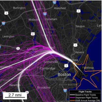
The modernization of aircraft navigation has meant that aircraft are able to fly designed flight tracks more precisely. This has led to a concentration of flights over the communities along the flight tracks. Communities at airports in many countries have cited the concentration in flight tracks as an increasing noise issue because of the frequent overflights above specific areas [3][4][5]. Figure 3 shows the flight track concentration and the increase in complaint locations following the implementation of RNAV, where the blue lines represent the departure tracks, the yellow lines represent the arrival tracks, and the red dots represent the complaint locations. Figure 3(a) shows the data from 2010, which was prior to the implementation of RNAV, and the flight tracks are dispersed. Figure 3(b) shows the data from 2017, which was after the implementation of RNAV, and the flight tracks are concentrated and there appear to be geographic areas of complaint locations associated with the RNAV procedures.

In order to understand the impacts of frequent overflights, metrics for assessing the annoyance mechanism were necessary. The metric for defining significant noise level in United States policy is annual average day-night average sound level (DNL) at 65dB [6]. However, the annual average DNL at 65dB does not appear to be representative of the complaint locations. In Figure 3(b), the white contour is the annual average DNL contour at the 65dB level at BOS in 2017 and only 1.2% of the of the complaint locations are within the contour. Therefore alternate metrics for assessing the impacts of frequent overflights were investigated in this thesis.

Metrics for assessing the impacts of frequent overflights allow for analysis of concepts for dispersed flight tracks. In many cases, the idea of returning to an airspace environment similar to pre-RNAV conditions with dispersed flight tracks is a politically attractive idea. However, the community noise impacts of dispersion are complex due to redistribution issues, and the implementation of dispersion may also be difficult for technical reasons. Figure 4 illustrates the need to have communication tools and visualizations to present noise analysis to communities, in order to support the community decision processes.

Figure 4. Need for Noise Metrics to Communicate Analysis Results to Allow for Community Decision Process [7]

The objectives of this thesis were, firstly, to determine a noise metric which is representative of the impacts of numerous overflights and, secondly, to analyze the potential impacts of dispersed flight tracks and various methods of communicating these results to stakeholders. Integrated exposure noise metrics of DNL and Nx were considered. The representative days of annual average day and peak day were also compared. Varying ways of communicating the analysis data to the communities have been presented in stakeholder meetings and will be discussed in this thesis.

Chapter 2

Background

2.1 Noise Metrics

2.1.1 Sound Pressure Level

Noise is defined as undesirable sound, and sound is caused by fluctuating pressure waves [8]. One of the most fundamental metrics for noise is sound pressure level (SPL), shown in Equation 1, where the reference pressure, Pref, is 20 μPa root mean square and P0 is the pressure amplitude of the sound wave [9]. SPL is a logarithmic metric so the units of measurement are decibels (dB).

𝑆𝑃𝐿 = 20 log₁₀( 𝑃0 𝑃_𝑟𝑒𝑓)

Equation 1. Sound Pressure Level

2.1.2 Frequency Weighting

Humans respond to some noise frequencies more so than others, therefore weightings are applied to certain frequencies in sound pressure level for specific noise metrics. Weightings are applied by dividing frequencies into 1/3-octave bands and then increasing or reducing the sound pressure level by a factor. Common weightings include A-weighting and C-weighting; Figure 5 plots A-weighting, represented as the blue line, and C-weighting, represented as the magenta line. A-weighting is used in aircraft noise overflights studies and heavily weights the mid-range frequencies of 2,000-6,000 Hz, as this is the range of most human speech and is the range where the human ear is most sensitive [10].

Figure 5. A-weighting and C-weighting Adjustment Curves [10]

2.1.3 Single Event Metrics: LA,max and Sound Exposure Level

While SPL is a measurement of instantaneous noise, additional metrics are used to communicate the overall noise level of an aircraft overflight. Figure 6 illustrates the metrics of LA,max and Sound Exposure Level (SEL). LA,max is the maximum A-weighted sound pressure level of an overflight. In Figure 6, the LA,max is the peak noise during the time of the overflight. SEL takes into account the duration of an overflight. SEL is calculated by integrating the weighted noise over time between the time when the A-weighted noise has risen to 10dB below the LA,max to the time when the A-weighted noise has fallen to 10dB below the LA,max. In Figure 6, the SEL is the gray area shaded integration area. [11]

Figure 6. LA,max and Sound Exposure Level [11]

2.1.4 Integrated Exposure Metrics: Day-Night Average Sound Level and Number Above

In order to quantify the noise effects of multiple overflights, integrated exposure metrics are used. A commonly used integrated exposure metric is day-night average sound level (DNL). DNL is a summation of SEL that is then averaged over the time period of a day, 86,400 seconds. A 10dB penalty is applied to night time overflights, which occur between 10pm and 7am. The calculation for DNL is shown in Equation 2 [12].

Equation 2. Day Night Average Sound Level [12]

Another integrated exposure metric is Nx. Nx is a count of the number of overflights above a certain LA,max threshold. The x indicates the day time LA,max threshold

and then the night time threshold has a 10dB LA,max penalty [13]. Figure 7 illustrates an example of how N60 would be calculated.

Figure 7. N60 Calculation

2.2

Literature Review

2.2.1 Annual Average DNL

One of the most commonly used noise metrics is annual average DNL at 65dB as this is the metric used to define significant noise exposure in United States policy. This threshold was adopted into regulation with the passing of the Aviation Safety and Noise Abatement Act of 1979. Annual average DNL at 65dB is the basis of billions of dollars in programs including sound insulation for homes and schools within the impact area of

of social surveys on noise annoyance” in 1978. In his study, Schultz uses responses to surveys as the basis for quantifying how annoyed people are by noise [14].

2.2.2 Number Above

Since 1978, studies have been conducted on additional metrics to communicate noise impacts aside from DNL. Southgate published in 2011 “The Evolution of Aircraft Noise Descriptors in Australia over the Past Decade.” One of the metrics that has gained increasing popularity in Australia as well as other countries is, as Southgate describes, ‘Number Above’ N70 [15]. N70 was chosen because this was taken to correlate with the sound level of a conversation 60dB inside an insulated home [16], however there is increasing interest in other noise levels for the number above metric as indicated in other studies.

2.2.3 Alternative Representative Days

In the United Kingdom “Survey of noise attitudes 2014: Aircraft” N70 is determined to be a useful supplemental metric. Other noise levels are also considered for the number above metric including N65. Another point of note from this publication is that the annual average day is not the only representative day considered. In this publication, the representative day of an average summer day is also considered relating to the idea that some days are more representative of the annoyance mechanism to communities than the annual average day [17].

Chapter 3

Noise Modeling Methodology

In order to determine the noise impacts to communities to assess various noise metrics, a noise modeling framework was necessary. Figure 8 shows the noise modeling methodology used in this study. The noise modeling program used was the Federal Aviation Administration (FAA) standard tool the Aviation Environmental Design Tool (AEDT) [18].

Figure 8. Noise Modeling Framework

Radar data includes information on the aircraft flown, which is then sorted into types of representative aircraft vertical flight profiles. The types of representative aircraft vertical flight profiles are shown in Table 1, which are B773 representing twin aisle jets, B757, A320, B738, MD88 representing older jets, E170 representing large regional jets, and E145 representing small regional jets. Brenner and Hansman also discuss the sorting of vertical flight profiles into aircraft bins as shown in Table 1 [19] and the full list for how aircraft are sorted into aircraft type bins is provided in Appendix A.

Table 1. Representative Aircraft Vertical Flight Profiles [19]

Representative Aircraft Type Category Name Category Description

B773 TA Twin Aisle Jet

B752 B757 Boeing 757 Family

A320 A320 Airbus A320 Family

B738 B737 Boeing 737 Family

MD88 OJ Older Jet

E170 LRJ Large Regional Jet

E145 SRJ Small Regional Jet, Business Jet, and Turboprop

-- PNJ

UNK

Excluded

(Piston Engine and Unknown)

On arrivals, the standard profiles from the noise modeling program AEDT were input into the noise model as the representative vertical flight profile for each aircraft type. For departures, the representative aircraft vertical flight profiles were generated by analyzing the altitude and speed data for each aircraft type and determining the median altitude and speed profiles. Using the median altitude and speed profiles from the data for each aircraft type, the thrust profile was calculated using the aircraft performance model BADA4. Thomas and Hansman [20] provides details on the vertical flight profile generation.

Radar data was also used to define each horizontal flight track. The data on the time of each operation was later used in calculating the integrated exposure metrics in determining if an overflight should be counted as a day time flight or a night time flight. In this study each radar data horizontal flight track was modeled individually.

The vertical flight profile data and the horizontal flight track data were then input into the noise model AEDT. AEDT output the results for a single event noise metric, in this case either LA,max or SEL. AEDT output the results in a grid format which could be matched with latitude and longitude. The noise results and the grid were then mapped onto a grid with population data from the 2010 census. Jensen and Hansman describes in further detail the population grid data from the 2010 census [21]. AEDT was run numerous times to represent each operation and then the noise results were aggregated on

the population grid to calculate the integrated exposure metrics, Nx or DNL, for the analysis in this study.

Chapter 4

Representative Averaging Day of Peak Day

During stakeholder meetings, communities often expressed an annoyance mechanism that was different from the annual averaging that is applied for a day in commonly used noise metrics. Complaints were often correlated with high intensity use periods; a community member might complain that there was a flight over his/her house every 90 seconds on a day starting at 6am. Therefore noise metrics were investigated during high intensity use periods in this thesis. Peak day will be further discussed in the following section and was investigated for both Nx and DNL.

4.1 Peak Day Identification

In order to capture the time period of high intensity use, it was necessary to determine a representative high utilization period. The peak day is defined as the day in a year during which a runway procedure had the most number of operations. The airports analyzed in this study were BOS, MSP, LHR, and CLT. The peak day was analyzed for the runway procedures at these airports. Further details on the airports and specific runway procedures analyzed in this study are discussed in Chapter 5. Table 2 compares the number of operations represented by the annual average day to the number of operations on a peak day for each of the runway procedures and airports analyzed in this study. Since runway configuration varies from day to day based on several factors including wind, there are days where a runway procedure has hundreds of operations and days where a runway procedure has no operations. Communities have expressed that the complaints are a result of the days on which there are hundreds of overflights over their homes, hence why the peak day was used as the representative time frame in the following analysis.

Table 2. Annual Average Day Operations vs Peak Day Operations*

Procedure

Annual Average Day Operations

Peak Day

Operations Peak Day BOS 33L dep 116 487 May 18th, 2017 27 dep 71 345 September 18th, 2017 4L/R arr 129 567 October 12th, 2017 MSP 17 dep 174 421 August 25th, 2017 30L dep 151 394 July 13th, 2017 12L/R arr 239 677 July 25th, 2017 30R dep 128 302 June 15th, 2017 LHR 9R dep 125 690 July 17th, 2017 27L/R arr 526 696 June 30th, 2017 CLT 18L/C/R arr 258 806 May 4th, 2017 18C dep 156 439 April 4th, 2017 18L dep 185 503 April 26th, 2017 36R arr 146 343 October 12th, 2017

*Note: Operations for parallel runways are the sum of all operations on the parallel runways.

Chapter 5

Correlation of Complaint Locations with

Runway Use

In order to analyze the noise impact of the peak day of each runway procedure, it was necessary to identify areas of impact associated with each runway procedure. Complaint location data was used in this study for the sole purpose of understanding the spatial extent of noise impacts of runway procedures. Complaint data was provided by the airports in this study. The complaint data set is all the complaints in 2017.

Multiple complaints from the same location are only counted as one complaint location, in order to gain an understanding of the distribution of complaint locations without being skewed by hypersensitive individuals. In the noise metric analysis, the goal is not to represent within the noise contour 100% of the complaint locations since there are hypersensitive complainants. Rather the goal of the noise metric analysis is to represent within the noise contour between 80% to 90% of the complaint locations.

To associate complaint locations with specific runway procedures, the complaint location data was clustered using a k-means algorithm. Cluster seeds were assigned along the approach and departure paths to determine if unique clusters of complaints could be identified for each runway. The cluster seeds were assigned 6.5nmi from the Airport Reference Point (ARP) along the approach and departure paths, as shown in Figure 9 through Figure 12. The distance 6.5nmi was observed to be the distance which was sufficient to uniquely define individual runway procedures while still within the area of significant complaints. The k-means algorithm logic assigned complaint location data to the cluster seeds, which serve as centroids, and then calculated the distance from each complaint location to the cluster centroid; the algorithm iterated under the cluster assignments did not change [22].

The complaint location clusters were then identified by runway procedure. Clusters were only correlated if uniquely defined by a single runway procedure. Clusters over low population density areas where the sample size was small and less than one hundred complaint locations were observed were not considered in this analysis. The following subsections describe the complaint locations clusters analyzed in this study; in

the following figures, the magenta diamonds represent the cluster seeds, the yellow lines represent the arrival paths and the cyan lines represent the departure paths.

5.1 BOS Clusters

At BOS the identifiable clusters of impact are 33L departures, 27 departures, and 4L/R arrivals. The non-identifiable and confounded clusters of impact are generally to the east of the airport near the harbor where both arrival and departure routes are present. Figure 9 shows the radar data and the clusters of impact for BOS in 2017, with 33L departures complaint locations shown as yellow dots, 27 departures complaint locations shown as orange dots, and 4L/R arrivals complaint locations shown as red dots; the non-identifiable and confounded clusters of complaint locations are represented by the white dots to the east of the airport.

5.2 MSP Clusters

At MSP the identifiable clusters of impact are 30R departures, 12L/R arrivals, 30L departures, and 17 departures. The non-identifiable clusters of impact are generally to the east of the airport which is much less population dense than the northwest of the airport, so the clusters were not used in the Nx analysis due to the small sample size. There is also a non-identifiable cluster of complaint locations to the south of the airport which appears to be caused by both 17 departures and 35 arrivals. MSP uses RNAV approach procedures but does not use RNAV departure procedures. Figure 10 shows the clusters of impact and radar data for MSP in 2017, with 30R departures shown as green dots, 12L/R arrivals shown as magenta dots, 30L departures shown as orange dots, and 17 departures shown as red dots; the clusters of complaint locations that were not used for the Nx analysis are shown as white dots and gray dots.

5.3 LHR Clusters

At LHR the clusters of complaint locations used in the Nx analysis are the 09 departures and the 27 arrivals to the east of the airport. The west of the airport is much less population dense so the clusters of complaint locations to the west of the airport were not used in the Nx analysis due to the small sample size. The complaint location data is from the “2017 Noise Complaint Report” for LHR [23]. Figure 11 shows the clusters of impact and radar data for LHR in 2017, with the 09 departures shown as orange dots, the 27 arrivals shown as blue dots; the clusters of complaint locations that are not used are the 27 departures shown as white dots and the 09 arrivals shown as red dots.

5.4 CLT Clusters

At CLT the identifiable area of impact is 18L/C/R arrivals. Additional clusters of impact seem to be correlated with 18C departures and 18L departures or 36R arrivals. Figure 12 shows the complaint location clusters and radar data for CLT in 2017; the 18L/C/R arrival complaint locations are shown as green dots, the 18C departure complaint locations are shown as red dots, and the cluster of complaint locations that appears to be correlated with either 18L departures or 36R departures is shown as blue dots.

Chapter 6

Annoyance Noise Threshold Determination:

Peak Day N

Parametric analysis was performed in order to determine the noise thresholds for the Nx metric. The sound levels of N55, N60, and N65 were analyzed, representing daytime thresholds of LA,max 55dB, 60dB, and 65dB and nighttime thresholds of LA,max 45dB, 50dB, and 55dB. The number of overflights was also swept through 25 overflights, 50 overflights, and 100 overflights for each sound level.

The results of the parametric sweep of N55, N60, and N65 for 25, 50, and 100 overflights are shown in Table 3 through Table 5 and are described in further detail in the following sections. The cells of the table were highlighted as red if less than 60% of the complaint locations were represented by the noise contour. Cells were highlighted as yellow in the results table if between 60% to 80% of the complaint locations were represented by the noise contour. Cells were highlighted as green in the results tables if greater than 80% of the complaint locations were represented by the noise contour.

Table 3. Peak Day N55 25 N55 50 N55 100 N55 BOS 33L dep 91.9% 89.5% 84.4% 27 dep 97.6% 95.7% 92.9% 4L/R arr 98.3% 95.8% 86.1% MSP 17 dep 98.1% 94.8% 85.2% 30L dep 95.7% 94.1% 82.6% 12L/R arr 95.5% 90.7% 85.8% 30R dep 97.7% 94.4% 84.9% LHR 9R dep 96.1% 94.3% 84.2% 27L/R arr 96.6% 92.4% 88.0% CLT 18L/C/R arr 85.3% 83.5% 82.6% 18C dep 77.2% 67.3% 48.8% 18L dep 69.0% 55.5% 18.6% 36R arr 39.5% 11.2% 9.1%

Table 4. Peak Day N60 25 N60 50 N60 100 N60 BOS 33L dep 87.3% 80.9% 59.4% 27 dep 95.4% 92.1% 78.8% 4L/R arr 97.7% 94.7% 81.0% MSP 17 dep 90.3% 83.2% 53.5% 30L dep 92.7% 83.1% 55.7% 12L/R arr 85.4% 77.6% 70.7% 30R dep 91.9% 87.2% 69.4% LHR 9R dep 91.0% 82.6% 61.4% 27L/R arr 93.2% 84.9% 80.2% CLT 18L/C/R arr 83.5% 80.7% 59.6% 18C dep 53.1% 34.0% 13.6% 18L dep 9.7% 7.1% 6.2% 36R arr 9.7% 7.4% 3.5%

Table 5. Peak Day N65 25 N65 50 N65 100 N65 BOS 33L dep 71.5% 51.0% 24.0% 27 dep 90.8% 78.3% 43.1% 4L/R arr 72.1% 65.2% 43.2% MSP 17 dep 69.7% 41.9% 5.2% 30L dep 74.9% 50.0% 28.3% 12L/R arr 72.4% 59.3% 45.1% 30R dep 78.0% 63.6% 29.2% LHR 9R dep 76.0% 57.1% 29.2% 27L/R arr 84.0% 72.4% 65.8% CLT 18L/C/R arr 78.9% 26.6% 4.6% 18C dep 17.9% 6.2% 3.7% 18L dep 6.2% 5.9% 3.2% 36R arr 7.1% 3.2% 1.8%

6.1 Noise Level Threshold

The sensitivity of each noise level is indicated by the results of the parametric sweep. N55 is shown in Table 3 to be too sensitive since there is little discrimination in the represented area between the 25 overflights threshold to the 100 overflight threshold. N65 is shown in Table 5 to be not sensitive enough since even at 25 overflights, the noise

metric under-represents the complaint locations and thus the impacted area. N60 is shown in Table 4 to have reasonable sensitivity to reflect changes in the impacted area based on changes in the number of overflights.

6.2 Overflight Count Threshold

Given that peak day N60 was the sensitivity level to count as an overflight, the number of overflights was also parametrically varied. As shown in Table 4, peak day N60 with 25 overflights is shown to over-represent the impacted area, while peak day N60 with 100 overflights is shown to under-represent the impacted area; however several procedures at CLT appear to be anomalous. N60 on a peak day with 50 overflights is shown to capture the majority but not all of the impacted area, thus representing the goal of 80% to 90% of complaint locations for each runway procedure area of impact.

6.3

Peak Day N

Overflight Contours

Because N60 was seen as the most diagnostic noise level, the N60 contours were further evaluated at each airport. Figure 13 through Figure 25 show the N60 contours for each of the airports and runway procedures in this study. The contours represented are the peak day N60 contours at 25 overflights, 50 overflights, and 100 overflights. The complaint locations associated with each runway procedure are represented by the red dots. The peak day flight tracks are represented as gray lines.

6.3.1 BOS

At BOS the analyzed runway procedures are 33L departures, 27 departures, and 4L/R arrivals shown in Figure 13 through Figure 15. The 33L departures in Figure 13 are a good visual example of the varying overflight levels for the N60 metric. The 100 overflight contour for N60, the innermost contour, appears too small for the representative area. The 25 overflight contour for N60, the outermost contour, appears to represent too

Figure 15. BOS 4L/R Arrivals Peak Day N60 at 25, 50, and 100 Overflights

6.3.2 MSP

At MSP the analyzed runway procedures were 17 departures, 30L departures, 12L/R arrivals, and 30R departures, shown in Figure 16 through Figure 19. At MSP, RNAV departures have never been implemented, however the threshold of N60 on a peak day with 50 overflights still appears to be a representative metric of impact. On the 12L/R arrivals, the 50 overflights at the N60 level on a peak day does not quite capture at least 80% of the complaints, however this could be due in part to confounding during the clustering process because the 12L/R arrivals have some overlap with the 30L and 30R departures.

6.3.3 LHR

At LHR analysis was performed on 9R departures and 27L/R arrivals, shown in Figure 20 and Figure 21. LHR has a runway use plan for noise purposes, so 9L is not used for departures. The metric 50 overflights on a peak day at the N60 level represents at least 80% of the complaint locations for the two runway procedures to the east of the airport. The west of the airport is a low population area causing a small sample size, while the east of the airport is a high population area being near London. It is worth noting that the metric of 50 overflights on a peak day at the N60 level appears to be a valid metric both within the United States and in another country.

Figure 21. LHR 27L/R Arrivals Peak Day N60 at 25, 50, and 100 Overflights

6.3.4 CLT

The results for CLT 18L/C/R arrivals are consistent with other airports, shown in Figure 22, where 50 overflights on a peak day at the N60 level represents at last 80% of complaint locations. However the communities to the south of the airport do not appear to reflect this pattern.

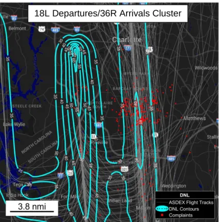
For the 18C departures, shown in Figure 23, there seems to be some possible effect from the turn, and this is also a low population density area. To the southeast of the airport, there is confounding of noise impacts because both 18L departures and 36R arrivals fly over this community, however a significant number of the complaints to the southeast of CLT are outside of the N60 contours even down to the 25 overflight level indicating a higher level of sensitivity, as shown in Figure 24 and Figure 25.

Figure 24. CLT 18L Departures Peak Day N60 at 25, 50, and 100 Overflights

18L Departures/36R Arrivals Cluster 18L Departures/36R Arrivals Cluster

6.3.4.1 CLT Peak Day N50

In order to further understand the anomalous runway communities at CLT, peak day Nx was also analyzed at the lower noise level of N50 for those communities. Table 6 shows the results of the peak day N50 analysis for the anomalous runway communities at CLT. The results indicate that the anomalous runway communities at CLT appear to be 10dB more sensitive to noise than all the other runway communities analyzed in this thesis. The fact that the overflight count sensitivity still appears to be 50 overflights thus further supports the idea that the anomalous runway communities at CLT are more sensitive in regards to the noise threshold. The peak day N50 results also indicate that the cluster of complaints to the southeast of CLT are primarily caused by 18L departures rather than 36R arrivals. Figure 26 through Figure 28 show the peak day N50 contours at the levels of 25 overflights, 50 overflights, and 100 overflights for the anomalous runway communities at CLT.

Table 6. CLT Peak Day N50

25 N50 50 N50 100 N50

CLT

18C dep 84.6% 82.1% 75.3%

18L dep 87.6% 82.6% 64.6%

Figure 26. CLT 18C Departures Peak Day N50 at 25, 50, and 100 Overflights

Figure 28. CLT 36R Arrivals Peak Day N50 at 25, 50, and 100 Overflights

6.4

Discussion

The threshold of peak day N60 with 50 overflights appears to represent the annoyance mechanism of frequent overflights at BOS, MSP, LHR, and one runway at CLT. However, the communities to the south of CLT appear to have increased noise sensitivity and a different noise threshold for annoyance impacts. CLT is the only airport that implemented RNAV departures and then implemented dispersed departures [24]. The communities experiencing the changes to the RNAV procedures have shown increased political sensitivity [25]. Part of the motivation for the analysis in this study is to have a metric for analyzing dispersed flight tracks, as communities have requested. However the CLT example begs the question of whether or not dispersed flight tracks will really have the desired effects.

Chapter 7

Annoyance Noise Threshold Determination:

Peak Day DNL

As an alternative to the Nx metric, evaluating DNL on a peak day could be considered. Table 7 through Table 10 show the analysis for peak day DNL. Peak day DNL was analyzed at the noise levels of 35dB to 75dB in 5dB increments. The cells of the table were highlighted as red if less than 60% of the complaint locations were represented by the noise contour. Cells were highlighted as yellow in the results tables if between 60% to 80% of the complaint locations were represented by the noise contour. Cells were highlighted as green in the results tables if greater than 80% of the complaint locations were represented by the noise contour. In order to capture more than 80% of complaint locations, the noise level of peak day DNL at 45dB is necessary, except for the anomalous runways at CLT.

In discussions with community stakeholder groups, it was found to be difficult for the communities to separate peak day DNL from the traditional annual average DNL. The use of peak day DNL at 45dB is both a different representative day and a different noise threshold from the metric that people are most used to seeing due to United States policy. DNL is also a logarithmic metric and can be more difficult to use to communicate impacts of procedures to communities compared to an arithmetic metric. For these reasons the peak day Nx metric is preferred over the peak day DNL metric in communicating analysis results with stakeholders, i.e. regarding dispersion,

Table 7. BOS Peak Day DNL BOS 33L dep 27 dep 4L/R dep Peak Day DNL Peak Day DNL Peak Day DNL 35dB 98.3% 99.8% 99.9% 40dB 96.3% 98.8% 98.7% 45dB 91.4% 95.5% 92.9% 50dB 64.1% 84.9% 73.1% 55dB 20.1% 44.6% 45.1% 60dB 7.2% 4.2% 5.4% 65dB 2.1% 3.0% 0.0% 70dB 0.1% 0.0% 0.0% 75dB 0.0% 0.0% 0.0%

Table 8. MSP Peak Day DNL MSP 17 dep 30L dep 12L/R arr 30R dep Peak Day DNL Peak Day DNL Peak Day DNL Peak Day DNL 35dB 100.0% 96.8% 98.8% 98.4% 40dB 98.7% 95.9% 95.5% 97.7% 45dB 83.9% 90.0% 89.8% 90.0% 50dB 39.4% 56.8% 76.4% 65.9% 55dB 0.0% 13.5% 42.0% 15.5% 60dB 0.0% 0.9% 0.0% 4.4% 65dB 0.0% 0.0% 0.0% 0.0% 70dB 0.0% 0.0% 0.0% 0.0% 75dB 0.0% 0.0% 0.0% 0.0%

Table 9. LHR Peak Day DNL LHR 9R dep 27L/R arr Peak Day DNL Peak Day DNL 35dB 96.8% 100.0% 40dB 96.7% 99.4% 45dB 92.5% 94.9% 50dB 69.8% 84.8% 55dB 32.4% 71.6% 60dB 0.7% 45.5% 65dB 0.0% 1.0% 70dB 0.0% 0.0% 75dB 0.0% 0.0%

Table 10. CLT Peak Day DNL CLT

18L/C/R

arr 18C dep 18L dep 36R arr

Peak Day DNL Peak Day DNL Peak Day DNL Peak Day DNL 35dB 91.7% 85.8% 88.5% 79.1% 40dB 87.2% 82.1% 68.1% 28.9% 45dB 82.6% 66.0% 8.8% 9.1% 50dB 80.7% 14.8% 6.2% 6.2% 55dB 17.4% 3.7% 1.8% 2.4% 60dB 0.0% 0.6% 0.0% 0.9% 65dB 0.0% 0.0% 0.0% 0.0% 70dB 0.0% 0.0% 0.0% 0.0% 75dB 0.0% 0.0% 0.0% 0.0%

7.1

Peak Day DNL Contours

Figure 29 through Figure 41 show the peak day DNL contours for the airports and runway procedures in this study. The outermost contour is the 35dB peak day DNL contour and then each contour increments by 5dB. The gray lines are the peak day radar flight tracks, and the red dots are the complaint locations.

7.1.1 BOS

At BOS, the peak day DNL at 45dB captures at least 80% of the complaint location for 33L departures, 27 departures, and 4L/R arrivals as shown in Figure 29 through Figure 31. In these figures for BOS, the peak day DNL at 45dB is shown as a magenta contour.

7.1.2 MSP

At MSP, the peak day DNL at 45dB represents at least 80% of the complaint locations for 17 departures, 30L departures, 12L/R arrivals, and 30R departures as shown in Figure 32 through Figure 35. The threshold of peak day DNL at 45dB is representative of the complaint locations for both the dispersed departures and for the RNAV arrivals at MSP.

Figure 35. MSP 30R Departures Peak Day DNL Contours

7.1.3 LHR

At LHR, peak day DNL at 45dB is representative of at least 80% of the complaint locations for both 9R departures and 27 arrivals, as shown in Figure 36 and Figure 37.

7.1.4 CLT

At CLT, peak day DNL at 45dB is representative of at least 80% of the complaint locations for 18L/C/R arrivals, as shown in Figure 38. However, this is not true for the anomalous runway procedures 18C departures, 18L departures, and 36R arrivals, as shown in Figure 39 through Figure 41. If the lower noise level of peak day DNL at 35dB is used, then at least 80% of the complaint locations are represented for the three anomalous runways. This analysis further supports the idea also shown in the Nx analysis that the CLT neighborhoods are 10dB more sensitive than the other airports and runway procedures analyzed in this study.

Figure 39. CLT 18C Departures Peak Day DNL Contours

Figure 41. CLT 36R Arrivals Peak Day DNL Contours

Chapter 8

Dispersion Analysis

Once peak day N60 with 50 overflights had been determined as the metric to communicate impact threshold, methods of modeling dispersion were investigated. Peak day DNL could have also been a defendable choice of metric to communicate the results of dispersion analysis; however for the reasons described in Chapter 7, peak day Nx is the preferred metric.

The dispersion analysis was completed for 33L departures and 27 departures at BOS, the two overland departure procedures. The examples will focus on 33L departures at BOS and the analysis for 27 departures at BOS is available in Appendix D.

8.1 Dispersion Analysis Communication Tools

The following tools were developed to communicate dispersion analysis results with stakeholders. In order to provide communities context for understanding the impacts of the changes due to RNAV, a comparison between pre-RNAV conditions and RNAV conditions was analyzed. The pre-RNAV to RNAV comparison was analyzed by comparing the 2010 conditions with the 2017 conditions, normalizing to the 2017 traffic levels as further described in following sections. The pre-RNAV to RNAV comparison for 33L departures will be used in the following sections as an example of the tools used to communicate dispersion analysis.

8.1.1 Population Exposure to N60 with 50 Overflights on a Peak Day

The overall impact of each dispersion concept was communicated by showing the number of people exposed to the metric of N60 on a peak day with 50 overflights. The population exposure numbers were calculated for the example of pre-RNAV to RNAV comparison, where the pre-RNAV flight tracks were normalized to match the RNAV traffic levels and fleet mix. The results of this analysis indicate that the RNAV conditions allow for a benefit of more than 12,000 people that are no longer exposed to the impact

to match the traffic levels of RNAV conditions, RNAV leads to an overall decrease in the number of people exposed to 50 overflights at the N60 level on a peak day.

Table 11. Population Exposure to N60 on a Peak Day with 50 Overflights for BOS 33L Departures Pre-RNAV to RNAV Conditions

8.1.2 Change in Peak Day N60 Maps

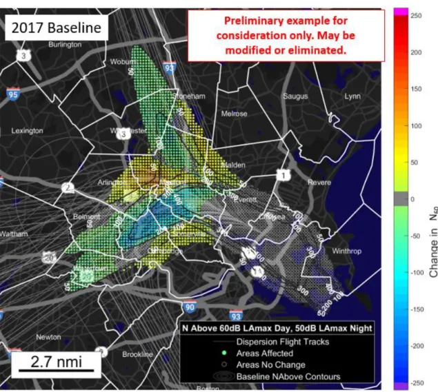
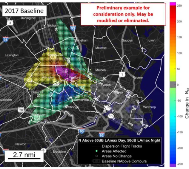
Maps are also shown to communicate the change in N60 on a peak day for the impacted areas. Figure 42 shows an example of the map used to communicate the change in N60 on a peak day when comparing pre-RNAV conditions to RNAV conditions.

The analysis is performed and communicated at the resolution of grid spacing that is 0.1nmi by 0.1nmi for each grid cell. This grid spacing allows for higher resolution than the census block level, which has previously been mentioned by stakeholders. Jensen and Hansman provides further detail on the population grid calculation method used [21].

The dots in warm colors indicate areas that will receive an increase on a peak day in N60 overflights as a result of the new procedure. The dots in cool colors indicate areas that will receive a decrease on a peak day in N60 overflights as a result of the new procedure. The white circles indicate areas that received no change or a change of less than an absolute value of 10 N60 overflights. If an area received an increase of greater than 250 overflights, then a dot was plotted in the color magenta. If an area received a decrease of more than 250 overflights, then a dot was plotted in purple. When RNAV was introduced, the areas under the RNAV tracks generally received an increase in overflights, while the areas under the previously dispersed flight tracks received a decrease in the number of overflights.

Information is also communicated about the absolute N60 overflight count. The N60 contours at 50 overflights, 100 overflights, 200 overflights, 300 overflights, and 400 overflights for the baseline conditions are plotted as dark gray contours over the colored dots. In Figure 42 this means that the baseline N60 contours are plotted for the pre-RNAV conditions, which have been normalized to the 2017 RNAV traffic levels. Additionally, dots are only plotted if they are within the impact threshold of 50 overflights at the N60 count for either the baseline conditions or the new procedure conditions. An ideal new procedure would be one which allowed for no new dots outside of the baseline contour at the 50 overflights at the N60 level.

The town boundaries are also provided on the map to allow decision-makers to understand how their specific constituents are impacted. The communication of town specific information will also be further discussed in Section 8.1.3.

8.1.3 Town by Town Analysis

In order to allow towns to further understand how their specific constituents are impacted, histograms were provided for each town showing the changes in N60 and the number of people who will receive that change. An example of these histograms are provided in Figure 43 for BOS 33L departures pre-RNAV to RNAV comparison. The columns in blue represent people who will receive a reduction in the number of N60 overflights, and the columns in red represent people who will receive an increase in the number of N60 overflights. All the dispersion histograms are provided in Appendix E.

Figure 43. BOS 33L Departures Pre-RNAV to RNAV Comparison Change in N60 Town Histograms

8.2

Peak Day Analysis for Dispersion Modeling

In order to model the noise impacts of dispersed flight tracks, the peak days of runway operations were analyzed. The peak day in 2017 for runway 33L departures at BOS was May 18th_{, 2017 on which day there were 487 departures from runway 33L. The} peak day in 2017 for runway 27 departures at BOS was September 18th_{, 2017 on which} day there were 345 departures from runway 27. The peak day for runway 4L/R arrivals at BOS was October 12th, 2017 on which day there were a total of 567 arrivals to the two runways. The peak day analysis on departures is described in this section, and further detail is given on the arrival dispersion analysis in Appendix C.

To analyze the peak day in further detail, the radar data was analyzed to determine the transition waypoint of the flight tracks, the type of aircraft being flown, and whether the aircraft was flying during day time or night time. The peak day analysis for runway 33L departures is shown as an example of how the analysis was performed. Runway 27 departures peak day analysis is shown in Appendix B.

The transition waypoint was determined by clustering the flight tracks at the point where the track distance travelled reached 15nmi. Figure 44 shows the runway 33L departure flight tracks sorted by their transition waypoints. The radar data was then further sorted, as shown in Table 12, to count the number of each type of aircraft and whether those aircraft were flying during the day, defined between 7am and 10pm, or during the night, defined as before 7am or after 10pm. Table 13 shows verification that the peak day was not an outlier in terms of numbers of procedures compared to the top five peak days of use for that runway.

Figure 44. BOS 33L Departures Peak Day Flight Tracks Clustered by Transition Waypoint

Table 12. BOS 33L Departures Peak Day Sorted by Transition Waypoint Clusters

8.3

Arrivals Dispersion

Dispersion was analyzed for both arrivals and departures as requested by the communities. However because of the design restriction of 15⁰ maximum final intercept angle for RNAV arrivals, the dispersion possibilities for arrivals are far more restricted. Rather than providing relief to the communities under the current arrival path, the possibilities for dispersion on arrivals were only able to move the noise to another part of the same community. Arrivals dispersion is discussed in Appendix C.

8.4 Altitude-Based Dispersion

For departure procedures that have a change in heading to the desired final track, one way to introduce dispersion is altitude-based dispersion. In the dispersion modeling, the aircraft flight tracks are routed direct to the transition waypoint once reaching the a chosen altitude, in this study either 3000ft or 4000ft. Because of the natural variability in aircraft climb rates, an example of which is shown in Figure 45, aircraft would reach the defined altitude at varying points along the ground and therefore be sent to the transition waypoint at different points thus introducing dispersion [26]. Figure 45 shows the natural variability in climb rates for B738 aircraft at BOS [27].

Figure 45. Natural Variability in Aircraft Climb Rates [27]

The flight tracks for BOS 33L departures altitude-based dispersion at 3000ft are shown as magenta lines in Figure 46. The flight tracks for BOS 33L departures altitude-based dispersion at 4000ft is shown in Figure 47. For all the following flight track figures, the dispersed flight tracks are shown as magenta lines. The white lines are the peak day radar data flight tracks. The orange contour is the annual average DNL at 65dB to show that the dispersion occurs outside of this threshold

Altitude-based dispersion at 3000ft for 33L departures at BOS results in an increase of over 5,000 people exposed to the impact threshold of 50 overflights at the N60 level on a peak day, as shown in Table 14. Figure 48 shows the change in N60 overflights for the areas impacted. In general the areas under the current RNAV tracks receive a reduction in the number of N60 overflights while the areas under the new dispersed flight tracks receive and increase in the number of N60 overflights.

Table 14. BOS 33L Departures Altitude-Based Dispersion at 3000ft Population Exposure to N60 with 50 Overflights on a Peak Day

Figure 48. BOS 33L Departures Altitude-Based Dispersion at 3000ft Change in N60 Overflights on a Peak Day

Altitude-based dispersion at 4000ft for 33L departures at BOS results in an over 62,000 person reduction in exposure to 50 overflights at the N60 level on a peak day. Altitude-based dispersion at 4000ft is effectively a concentration of flight tracks compared to the current RNAV flight tracks, since the flights stay along one track for a longer amount of time going west. The area further west of the airport is also less population dense thus resulting in the population exposure decrease. Figure 49 shows that while the people under the current RNAV tracks receive a significant reduction of about a 200 overflight reduction, the people under the westward track from the airport receive a significant increase in N60 overflights of over a 250 overflight increase at the N60 level.

Table 15. BOS 33L Departures Altitude-Based Dispersion at 4000ft Population Exposure to N60 with 50 Overflights on a Peak Day

Figure 49. BOS 33L Departures Altitude-Based Dispersion at 4000ft Change in N60 Overflights on a Peak Day

8.5 Controller-Based Dispersion

Controller-based dispersion was modelled based on pre-RNAV flight tracks that were normalized against RNAV flight tracks. Conversations with controllers indicated that this would be the closest model to controller-based dispersion. To model the pre-RNAV flight tracks and to make a fair comparison with the 2017 peak day, the 2010 peak day was analyzed and normalized against the 2017 data. Data was normalized by the aircraft destination direction and the type of aircraft, the day night counts were based on

the 2017 peak day data. Table 16 shows the 2010 and 2017 peak days analysis for BOS 33L departures, and the same analysis is shown for BOS 27 departures in Appendix B. If there were too many flight tracks represented on the 2010 peak day, then the appropriate number of flight tracks were randomly selected from the 2010 data; and if there were too few flight tracks represented on the 2010 peak day, then randomly selected flight tracks were counted twice. In Table 16, for northbound B757s only two of the flight tracks from 2010 were selected; and for northbound A320s, fifteen of the flight tracks were counted twice to represent the same number of northbound A320s as in 2017.

Table 16. BOS 33L Departures 2010 Peak Day Normalized Against 2017 Peak Day

The flight tracks for controller-based dispersion are shown in Figure 50. Table 17 shows that controller-based dispersion would result in an increase of over 12,000 people exposed to the impact threshold of 50 overflights at the N60 level on a peak day. Figure 51 shows that in controller-based dispersion, the southbound flights are often turned

Figure 50. BOS 33L Departures Controller-Based Dispersion Flight Tracks

Table 17. BOS 33L Departures Controller-Based Dispersion Population Exposure to N60 with 50 Overflights on a Peak Day

Figure 51. BOS 33L Departures Controller-Based Dispersion Change in N60 Overflights on a Peak Day

8.6 Divergent Heading Dispersion

Another approach would be to do programmed divergent headings of 15⁰ or greater depending on the trajectory. Divergent headings help to maintain aircraft separation requirements, since once the aircraft are on divergent headings of 15⁰ or

will follow on the runway and thus also help to maintain separation requirements. 15⁰ or greater divergent headings could be assigned based on the aircraft destination. In the divergent heading dispersion modeling, the aircraft are sent to the transition waypoint upon reaching 3000ft altitude [26]. The flight track modeling for 33L departures divergent heading dispersion is shown in Figure 52 where the dispersion flight tracks are shown as magenta lines.

Table 18 shows that the divergent heading dispersion concept would result in a 2,000 person reduction for the exposure to 50 overflights at the N60 level for the 33L departure communities at BOS. This is a result of the divergent heading flight tracks overflying less population dense areas. Figure 53 shows that there would be areas that would be newly exposed to noise due to the divergent headings.

Table 18. BOS 33L Departures Divergent Heading Dispersion Population Exposure to N60 with 50 Overflights on a Peak Day

8.7 RNAV Turning Waypoint Relocation

Dispersion could be introduced by changing the location of a turning waypoint, thus changing the location where RNAV procedures begin to branch. The concept was motivated by runway 27 departures at BOS where the introduction of RNAV also introduced a new waypoint that moved the turning waypoint further along the departure path and resulted in increased noise exposure to a population dense area. The idea is to move the waypoint back to the previous location prior to RNAV to provide relief to this community by allowing the departure paths to branch sooner. This idea is further discussed in the 27 departures analysis in Appendix D. For runway 33L departures at BOS, the choice of waypoint relocation is not as clear, so the analysis was done parametrically by moving the current fly-by waypoint closer to the airport 1nmi and 0.5nmi and also further from the airport 1nmi and 0.5nmi, as shown in Figure 54 through Figure 57.

Figure 57. BOS 33L Dep. RNAV Turning Waypoint Relocation Flight Tracks +1nmi

The population exposure numbers and the change in number of N60 overflights are shown in Table 19 through Table 22 and in Figure 58 through Figure 61. In general the areas further west from BOS are less population dense, so moving the waypoint further west results in a reduction in the number of people exposed to the impact threshold of 50 overflights at the N60 level. The figures showing change in N60 show that some of the waypoint relocations would result in more drastic changes in number of overflights, changes as great 250 overflights in magnitude. The parametric sweep of RNAV turning waypoint locations illustrates the sensitivity of population exposure to RNAV procedure design.

Table 19. BOS 33L Departures RNAV Turning Waypoint Relocation -1nmi Population Exposure to N60 with 50 Overflights on a Peak Day

Table 20. BOS 33L Departures RNAV Turning Waypoint Relocation -0.5nmi Population Exposure to N60 with 50 Overflights on a Peak Day

Figure 59. BOS 33L Departures RNAV Turning Waypoint Relocation -0.5nmi Change in N60 Overflights on a Peak Day

Table 21. BOS 33L Departures RNAV Turning Waypoint Relocation +0.5nmi Population Exposure to N60 with 50 Overflights on a Peak Day