Chaotic Advection and Mixing in a Western Boundary Current-Recirculation System: Laboratory Experiments
By
Heather E. Deese
B.S., Georgetown University, 1998
Submitted in partial fulfillment of the requirements of the degree of Master of Science
at the
MASSACHUSETTS INSTITUTE OF TECHNOLOGY and the
WOODS HOLE OCEANOGRAPHIC INSTITUTION February 2001
© 2000 Heather E. Deese All rights reserved.
The author hereby grants to MIT and WHOI permission to reproduce paper and electronic copies of this thesis in whole or in part and to distribute them publicly.
Signature of Author
/,/ Joint Program in Oceanography
Massachusetts Institute of Technology and Woods Hole Oceanographic Institution December, 28 2000 Certified by Larry Pratt , /
A
Thesis Supervisor Accepted by MASSACHUTEAP
1
yA
RIES
Chair, Carl Wunsch Joint Committee fbr Physical Oceanography Massachusetts Institute of Technology and Woods Hole Oceanographic InstitutionChaotic Advection and Mixing in a Western Boundary Current-Recirculation System: Laboratory Experiments
By
Heather E. Deese
Submitted to the Department of Earth, Atmospheric, and Planetary Sciences at MIT and the Department of Physical Oceanography at WHOI on December 28,2000 in partial fulfillment
of the requirements for the degree of Master of Science in Physical Oceanography.
Abstract:
I study the exchange between a boundary current and flanking horizontal recirculations in a 'sliced-cylinder' rotating tank laboratory experiment. Two flow
configurations are investigated: a single recirculation and a double, figure-8, recirculation. The latter case involves a hyperbolic point, while the former does not. I investigate the
stirring and mixing under both steady and unsteady forcing.
I quantify the mixing in each case using effective diffusivity, KC~, and a corollary effective length, Le, as derived by Nakamura (1995, 1996). This approach involves diagnosing the geometric complexity of a tracer field. Geometric complexity is indicative of advective stirring. Because stirring creates high gradients, flows with high advective stirring also have high diffusion, and stronger overall mixing. I calculate effective length from images of dye in the tank and find much higher values of Leff in the unsteady
hyperbolic cases than in the other cases.
Slight unsteadiness in flows involving hyperbolic points gives rise to a chaotic advection mechanism known as 'lobe dynamics'. These lobes carry fluid in and out of the recirculations, acting as extremely effective stirring mechanisms. I demonstrate the
existence of these exchange lobes in the unsteady hyperbolic (figure-8) flow. The velocity field in the tank is calculated utilizing particle image velocimetry (PIV) techniques and a time series U(t) demonstrates the (forced) unsteadiness in the flow. Images of dye in the tank show exchange lobes forming at this same forcing period, and carrying fluid in and out of the recirculation.
Based on the results of these experiments, I am able to confirm that, at least in this controlled environment, basic geometry has a profound effect on the mixing effectiveness of a recirculation. I demonstrate radically increased stirring and mixing in the unsteady hyperbolic flow as compared to steady flows and flows without hyperbolic points.
Recirculations are ubiquitous in the world ocean; they occur on a variety of scales, in many different configurations, and at all depths. Some of these configurations involve hyperbolic points, while others do not. Chaotic advection via lobe exchange may be an important component of the mixing at multiple locations in the ocean where hyperbolic recirculation geometries exist.
Thesis Supervisor: Larry Pratt
Title: Senior Scientist, Physical Oceanography Department, Woods Hole Oceanographic Institution
I. Introduction:
The motivation for this work came from the realization that some basic recirculation geometries associated with enhanced mixing due to chaotic advection appear in multiple locations in the oceans. Analytical and numerical studies of geometries involving
hyperbolic points have highlighted the importance of a chaotic advection mechanism known as 'lobe dynamics' (e.g. Rom-Kadart, et al. 1990, Wiggins 1992, and Miller, et al. 1997). Hyperbolic geometries arise wherever recirculations (of the same sign) occur next to each other. Exchange lobes arise whenever a flow with a hyperbolic point becomes slightly unsteady. These lobes carry fluid in and out of the recirculations, acting as extremely effective stirring mechanisms. Because stirring creates high gradients, flows with high advective stirring also have high diffusion, and stronger overall mixing. Lobe exchange
may be an important component of the mixing at multiple locations in the ocean where hyperbolic recirculation geometries exist.
Recirculations are ubiquitous in the world ocean; they occur on a variety of scales, in many different configurations, and at all depths. Some of these configurations involve hyperbolic points, while others do not. There appear to be a series of recirculations along the course of the Deep Western Boundary Current (DWBC)' in the North Atlantic and these were the particular features that sparked my interest. In some locations two or more
recirculations line the course of the DWBC, with hyperbolic points between each pair. These recirculations may have a profound effect on the path a parcel of deep water takes along the boundary (Fine, 1995). We would like to understand the effects of the
recirculations in order to more fully describe the information pathways and delay times in the abyssal oceans and their role in the Meridional Overturning Circulation (MOC). In addition to this particular deep application, many questions remain about the effects of surface or mid-depth recirculations in the oceans. I wondered whether I could say something about the mixing that would occur in the region of a recirculation based on whether or not the basic geometry involved a hyperbolic point.
I study the exchange between a boundary current and flanking horizontal
recirculations with and without hyperbolic geometries. Based on the results of a series of
I use 'dwbc' or 'dbc' to specify the general phenomenon of deep (western) boundary currents and 'DWBC' to specify the Deep Western Boundary Current in the North Atlantic.
laboratory experiments, I am able to confirm that, at least in this controlled environment, basic geometry has a profound effect on the mixing effectiveness of a recirculation.
I use a 'sliced-cylinder' rotating tank to produce the boundary current and
recirculations in the laboratory. The single layer of fluid displays a slow interior flow and a fast 'western' boundary current due to the stress of a differentially rotating lid and the topographic beta effect of a sloped tank bottom. At low lid rotation rates a single 'Munk' recirculation lies between the boundary current and the interior (Figure Ila). At higher forcing a second, 'inertial' recirculation forms 'north' of the first, resulting in a double recirculation, figure-8, geometry with a hyperbolic point (Figure Ilb). I investigate both
steady and unsteady cases (the unsteady cases are forced by adding a slight oscillation to the lid rotation).
I diagnose mixing in each case using effective diffusivity, ic' , and a corollary effective length, L , as derived by Nakamura (1995, 1996). This approach involves diagnosing the geometric complexity of a tracer field. Geometric complexity is indicative of advective stirring, and strong stirring results in increased diffusive mixing. This has been demonstrated numerically by Nakamura (1996) and employed by Nakamura and others to diagnose mixing in the atmosphere (Nakamura 1995, Nakamura & Ma 1997, Haynes & Shuckburgh 2000). In this work I calculate effective length from images of dye in the tank.
In addition, I demonstrate the underlying lobe dynamics that I believe account for the higher effective diffusivity in the flow with a hyperbolic point. The velocity field is calculated utilizing particle image velocimetry (PIV) techniques, and a time series U(t) demonstrates the (forced) unsteadiness in the flow. Images of dye in the tank show exchange lobes forming at this same forcing period, and carrying fluid in and out of the recirculation.
I am not attempting to model a particular geographical region, but instead to investigate generic flow geometries that occurs in many locations. (In the section on oceanographic observations I highlight the shared characteristics which contributed to our choice of geometries.) I do not investigate the cause of these deep recirculations, but rather attempt to elucidate their effects. I essentially create a model in the laboratory tank, and study the fundamental differences between two generic recirculation configurations.
My final goal is to learn something about the nature of exchange between the wbc, the recirculation(s), and the interior. What can I say about the mixing along the edges of
the recirculation(s)? Are particles more likely to exit back into the boundary current or into the interior flow to the east? How quickly and effectively do recirculations homogenize fluid trapped inside? How does altering the geometry of the recirculation region affect the mixing characteristics of the flow? What are the dynamics that underlie the mixing?
The rest of this work is presented in the following way. Sections II-III present background information and relevant oceanographic observations of the deep
recirculations. In section IV I outline the theory of lobe dynamics, which combined with the observations determined our choice of flow geometries. Section V includes
background information on our laboratory apparatus and procedures. The velocity calculation and dye pictures depicting the exchange lobes are presented in sections VI and VII, respectively. Section VIII contains the calculations of effective diffusivity, with further notes on the effects of the exchange lobes. In Section IX I summarize my findings and suggest directions for further work in the laboratory. In addition I briefly discuss the relevance to oceanographic situations and possible ways to incorporate the concepts of lobe dynamics and effective diffusivity into analysis of oceanographic observations.
Figure Il: Schematic illustration of the two recirculation configurations investigated. Panel a: a single recirculation lies between a western boundary current and an interior flow. In the laboratory this 'Munk' recirculation represents the non-hyperbolic case. Panel b: a double, figure-8, pair of recirculations. This is obtained in the laboratory in a flow regime where the Munk recirculation and an 'inertial' recirculation coexist. A hyperbolic point is visible where the streamlines outlining the recirculations intersect.
2~.
F~~uv~e.JTI
a
V
0~
II. Background:
Diagnosing the mixing around all types of recirculations is important, but
understanding the recirculations along the deep boundary currents is an especially difficult and significant problem. This is because the deep boundary currents and surrounding features comprise the lower branch of the Meridional Overturning Circulation (MOC)1. This circulation consists of the poleward transport of warm water near the surface and the
equatorward flow of cold water at greater depths. The transformation of this surface water into deep water requires rare atmospheric and oceanic conditioning, and thus occurs
sporadically and in only a few locations. It is the deep boundary currents that transport both this newly ventilated water and older deep waters throughout the world oceans.
The question of the content and characteristics of the deep transport system is
especially important because these deep currents carry information about the climate conditions at the time of their formation and will eventually feed back this information into the world's surface waters. As this water upwells thousands of years later it will affect all sorts of systems from biological communities to weather patterns and the global climate.2
We would like to understand the information pathways and delay times in the abyssal
oceans so that we can describe and predict the Meridional Overturning Circulation more completely.
One analogue to these laboratory experiments is the important, but little understood,
horizontal recirculations that flank the paths of the deep boundary currents. The most well-studied part of the deep ocean is the North Atlantic, and throughout this region
investigators have identified deep boundary currents lined by recirculations of various sizes (McCartney 1992, Schmitz & McCartney 1993, Johns, et al. 1997, Lavender, et al. 2000).
(see figures 01, 02, 03) Although for a combination of historical, political, social, and
economic reasons, much less work has been done in the other oceans, some of the observations along other dwbcs indicate similar patterns. (for Pacific flows see Wijffels, etal. 1998. For South Atlantic flows see Stephens & Marshall 2000 and Spall 1994)
I adopt Munk and Wunsch (1998) suggestion and use the term Meridional Overturning Circulation (MOC) instead of Thermohaline Circulation. The authors hold that since the forcing of this vertical overturning circulation is not necessarily exclusively thermohaline, the MOC is a more appropriate term.
2 The time it takes deep water to upwell and effect surface waters is still not well known, in the case of
some water that transits the world oceans, it could be much longer than 0(1000) years. For newly formed water in the 'shallow' branch of the DWBC, the time could be much less than 0(1000) years.
There are a number of ways in which recirculations may affect the transport of deep water and its interaction with other waters. Recirculations presumably modify both the time it takes a water parcel to move along the boundary and the exposure of that parcel to other water masses. Parcels of water which peel off from a wbc into a recirculation and spend some period of time 'trapped' there before returning to the core flow take a much longer time to move along the boundary. In addition they are exposed to a different mixing environment than they would have been otherwise; both the mixing intensity and
neighboring water masses are presumably different due to the presence of the recirculation (Fine 1995).
Recirculations could therefore explain the disparity between the travel time one expects along the boundary from direct current measurements and the age of the deep water
along its track as indicated by tracer fields (Fine, ibid.). Recirculations also seem to explain the regions of homogenized characteristics found at various locations alongside the
dbcs (Fine, ibid.). In addition, the spatial distribution of vertical mixing in the oceans is still largely unknown, and recirculations may play some role in determining that pattern. An extreme example arises in the mid-depth water of the Labrador Sea. Various
investigators have postulated that deep convection occurs in particular locations because water is trapped there for some time by horizontal recirculations. The air-sea dynamics
work more effectively on this trapped water, conditioning it for convection through cooling (Clarke & Gascard 1983 and Lavender, et al. 2000).
We would like to answer some basic questions about this type of recirculation. How much time is a parcel likely to spend trapped in a recirculation? Are trapped parcels more likely to end up exiting into the interior flow or into the boundary current? How
quickly and effectively do recirculations act to homogenize any fluid trapped inside? Do recirculations with certain underlying geometries tend to entrain and mix more than others? What are the mechanisms by which all of this exchange occurs? We must find answers to
these questions before we can build even a basic understanding of the deep branch of the meridional overturning circulation.
Diagnosing the rate of feedback via the deep transport system is especially
important because deep water formation is highly time dependent. For example, during the early 1990s there was extremely high production of Labrador Sea water in the northern North Atlantic. A series of observational studies have tracked this strong pulse of newly formed deep water as it has propagated down the course of the DWBC which hugs the
coast of North America (Curry, et al. 1998 and Molinari, et al. 1998). Others have investigated the interplay between this formation event and the variability in other deep water types (i.e. overflow water, etc. see Pickart, etal. 1999). While still others have investigated the connection between the strength of deep water formation and the strength of the overturning circulation (Mauritzen & Hakkinen 1999 and Munk & Wunsch 1998). In order to fully understand the long term affects of the time variability in the MOC we must be able to predict when anomalous signals will affect the surface properties of the oceans. This requires piecing together a better understanding of the deep transport system. If we clearly diagnose the delivery system, we may be able to develop powerful predictive capabilities.
III. Oceanographic Observations:
In terms of oceanographic observations I define a horizontal recirculation as a region where some offshore (or occasionally inshore) return flow transports water derived from the boundary current water as shown schematically in Figure II. In many cases deep recirculations have been postulated based on characteristics of the deep boundary current (dbc) in some region (i.e. otherwise inexplicable changes in transport and or tracer signals along a section of the boundary current). In most locations return flow has not yet been measured. In a few cases the return flow has been measured and I describe these cases below. This physical evidence is often bolstered by details of tracer distribution, which can
indicate recirculations where tracer signals characteristic of the boundary current stretch toward the interior. These signals can be interpreted as indicating the area of a recirculation adjacent to the boundary current (e.g. Fine and Molinari, 1988).
Tracer data has also indicated some large-scale effects which have been linked to recirculations. Namely, the tracer-derived ages for the Deep Western Boundary Current are much older than the time it would take a parcel to move along the boundary at the observed current velocities. In her review of relevant tracer measurements, Fine (1995) notes that the tracer-derived DWBC velocities are 0(1 cm/s) while the observed DWBC velocities are
0(10-50 cm/s). Despite high uncertainty in the tracer-derived ii, this order of magnitude difference indicates that either significant mixing or horizontal recirculation (or more likely, both) are involved in the transport of parcels along the boundary.
The deep recirculations seem to occur on a variety of scales and for various reasons. Many of the smaller 'meso-scale' recirculations, 0(100-400 km), appear to be due to interactions of the flow with local topography, but the dynamics of other meso-scale recirculations are mysterious. The larger, 'basin-scale' recirculations, 0(500-1000) km, fill many of the abyssal plains which comprise the deep ocean floor. In the North Atlantic, these abyssal plains typically stretch from the continental margin to the mid-ocean ridge in
the zonal direction and are bounded in the meridional direction by smaller ridges or other topographic barriers. In some locations there appear to be both meso-scale and basin-scale recirculations in play, with some dbc water recirculating close to the boundary and some recirculating much further from the boundary. In all of these locations there is some net throughflow along the boundary in the deep boundary current, but the characteristics of the water that exits the region may be strongly affected by the presence of the various
recirculations.
The majority of the observations recounted here supply indicative, but not
conclusive, evidence of recirculations. In a few cases, repeated sets of measurements of different kinds (moorings, hydrographic surveys, floats, and tracers) provide a
preponderance of evidence for recirculation along the DWBC. The most well documented case of a recirculation abutting a deep boundary current is in the Abaco region - 24-30N in the western Atlantic. I review the work in this region below, after summarizing some observations in other areas.
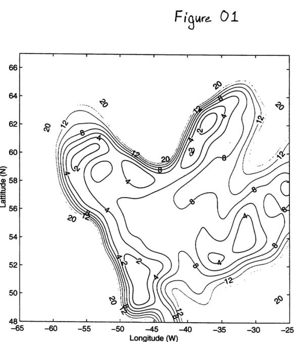
Recent work in compiling float data into Eulerian fields in the Irminger and Labrador Basins has highlighted meso-scale cyclonic recirculations that are embedded in the larger, basin-scale looping of the DWBC as it enters and leaves each basin (Lavender, et al. 2000). The streamlines of this flow are reprinted by permission in Figure 01. The authors were able to diagnose the mean, mid-depth, horizontal circulation by compiling drift results from 200 PALACE and SOLO floats at 400, 700, and 1500 m depth. The resulting velocity field contains a series of cyclonic recirculations with the return flow in the interior -1/4 the speed of the boundary currents, which is 12 cm/s maximum, and the total width of the recirculations is 0(1-2) times the width of the boundary current. The highest velocities and the only clear time dependence (an annual signal in the transport) occurred in the cyclonic gyre north of the Flemish Cap (50N, 47W) and the figure-eight pair of
recirculations east of Greenland (61N, 37W). Current meter results also show indications of return flows offshore of the Labrador and Greenland currents (Pickart, et al. 2000 and Clarke & Gascard 1983).
Lavender, et al. 2000 also note other phenomena associated with these
recirculations. This first is that deep mixed layers and sluggish velocities 0(1.5 cm/s) occurred during winter time in the region of a cyclonic recirculation in the western Labrador sea near 56.5N. This is a region where other investigators have found Labrador Sea Water
formation (Pickart, 1998). These results support the suggestion by Clarke and Gascard (1983) that deep water could be formed in a localized, offshore, cyclonic recirculation.
The second note is that extremely complex trajectories were found near the Flemish Cap. There are multiple flow components here, as the Labrador Current looping around the Cap from the north encounters the North Atlantic Current entering the region from the
southwest. The float trajectories from the middle and deep layers bifurcate in this region, some recirculating north back into the Labrador Sea, a number heading east towards the Mid-Atlantic Ridge, and one continuing south (presumably in the core of the DWBC). The
resulting "rapid exchange between the boundary current and offshore waters" (Lavender, et al. 2000, p.68) may be due to a hyperbolic point where the interior recirculation of the Labrador Sea encounters the larger-scale flow.
A number of basin-scale recirculations have been proposed, and some of these are shown schematically in Figure 02. I have sketched this cartoon based on the work
outlined below; I have reprinted the bottom topography (with permission) from McCartney (1992). Examples include a recirculation consisting of both DWBC water and Antarctic Bottom Water (AABW) in the Guiana basin and a series of recirculations of AABW and Iceland-Scotland Overflow Water (ISOW) in the basins of the eastern North Atlantic (Van Aken 2000; McCartney 1992; Johns, et al. 1993; Schmitz & McCartney 1993).
Investigators have proposed multiple explanations for the existence of these recirculations, including large-scale topographic beta effects, instability of the boundary current, and specified, non-uniform upwelling. (Nof & Olson 1993; Speer & McCartney 1992; Kawase 1993; Spall 1994).
McCartney (1992) employs hydrographic stations in the Madiera Basin to identify northward flow in the east at 2.2 Sv with a return flow southward in the west of 0.6 Sv, resulting in 1.6 Sv of throughflow of the coldest bottom water. Further north McCartney (1992) combines multiple hydrographic studies and a few current meter results in his diagnosis of 3.9 Sv flowing northward along the eastern edge of the West European basin with 1 Sv recirculating at the western edge of that basin.
Further work with inverse models (Gana and le Provost, 1993) and detailed water mass composition analysis (Van Aken, 2000) has bolstered the evidence for these cyclonic recirculations. Van Aken (2000) substantiates evidence for recirculations in Madiera and West European Basins by tracking the southward influence of ISOW (Iceland-Scotland
Overflow Water) as far south as the Madiera Basin at 30N, and proposes a similar feature in the Iberian Basin.
In addition to these large scale recirculations, the deep boundary current in the North Atlantic is characterized by huge meanders or intrusions into the subpolar basins. In all four northern basins (Rockall Trough, Iceland Basin, Irminger Basin, and Labrador Sea) McCartney (1992) identifies the signature of deep boundary current water looping in and out of the basins in a cyclonic manner. He does not identify these loops as closed recirculations, but more recent work indicates a closed recirculation is likely in the Iceland Basin (personal communication, Cecilie Mauritzen).
Another basin-scale recirculation (possibly made up of a series of recirculations) was predicted between the equator and 30N in the western Atlantic by Schmitz &
McCartney 1993. This would involve both NADW and AABW contributing to a cyclonic recirculation, with northward flow along the western flank of the mid-ocean ridge and southward flow (in the DWBC) along the continental margin. Observational work in progress (Guiana Abyssal Gyre Experiment, McCartney and Mauritzen, co P.I.s) aims at directly measuring the northward flow. There are also indications of basin-scale
recirculating components in the Canary Basin/Gambia Abyssal Plain and Brazil Basin. (Stephens & Marshall, 2000).
In addition to these deep recirculations, there are many surface intensified
recirculations, some of which have very deep signatures stretching almost throughout the entire water column. Examples include: the Great Whirl in the Gulf of Aden off Somalia, the Mann Eddy in the Newfoundland basin, the Alboran Gyre north of Morocco in the Mediterranean Sea, the inertial gyres that lie on either side of the Gulf Stream between Cape Hatteras and Grand Banks and a similar, but smaller, feature to the south of the
Kurishio. Many investigators have studied the recirculations on either side of the Gulf Stream, including the entrainment of the DWBC water as it passes through the region (Hogg, N.G. 1992, Spall 1996 (I&II), and Bower and Hunt 1999 (I&II)). The recirculations in this region are extremely complex due to the interaction of intense boundary currents traveling in different directions at different depths, and presumably involve a number of hyperbolic points, so that chaotic advection may play an important role in the regional mixing.
The Abaco area east of the Bahamas is a well studied region that demonstrates the complex structure of the DWBC. The results from a long-standing current meter array across the DWBC at 26.5N demonstrated a surprisingly high total transport which hinted at an offshore recirculation (Lee, et al. 1996). Additional work, in the form of hydrographic and chemical tracer surveys, PEGASUS current profiles, moored measurements,
dropsondes, and RAFOS floats, has refined our understanding of the circulation in this region (Fine & Molinari 1988; Leaman & Vertes 1996; Johns, et al. 1997). This work has elucidated meso-scale recirculations and hinted at basin-scale recirculations that contribute to the high mass flux along the boundary. The many types of measurements in this area have allowed investigators to state with confidence that this region is characterized by enhanced advective and diffusive mixing: "the DWBC recirculation gyres, and enhanced
mixing due to topographic influences, appear to be an effective means for ventilation of the interior and dilution of the DWBC tracer concentrations" (Johns, et al. 1997, p. 2206) Figure 03 presents approximate streamlines in the region showing the local, meso-scale recirculation (panel a from Johns, et al. 1997, reprinted with permission) and the bottom topography in the region (panel b from Leaman and Vertes, et al. 1996, reprinted with permission, I have added a bold line at the 4500m isobath).
Lee, et al. (1996) present the cumulative data of 5.8 years of moored current meter measurements from a section along 26.5 N. They calculate a total southward transport of 40 +/- 13 Sv (Sv = Sverdrup is defined as a million cubic meters) in the DWBC.' Of this total southward boundary flow, they approximate 27 Sv must recirculate somewhere in the western North Atlantic, as only 13 Sv is required to balance the Meridional Overturning Circulation at this latitude.
Johns, et al. (1997) detail the portion of this 27 Sv which is recirculated locally in a meso-scale recirculation (Figure 03a). This recirculation, which the authors diagnose as carrying 12 Sv, spins most strongly over a 'bump' in the bottom topography which is the southern extension of the Blake Bahama Outer Ridge (Figure 03b). This bump lies
This total transport was obtained by selectively removing data from periods when the DWBC was in an offshore position. Their moored array, which stretched to 85 km offshore for most of the 5.8 years, and to
125 km offshore for the last two year deployment, did not capture the full core of the DWBC during these offshore excursions. (They find the DWBC 'offshore' 32% of the time). They attribute these offshore excursions to interactions with westward propagating baroclinic Rossby waves with a period of 70-100 days. They also find inshore recirculations of northward flow during these periods when the DWBC is located further offshore 0(100 km).
between 74-74.5W and 26-29N. The cyclonic gyre stretches from 75.5W-74W (300 km) and from 25N-29.5N (500 km). Embedded within this recirculation are two smaller features 0(100 km) which transport 4-8 Sv each.
Tracer signals in the region also support the local recirculation hypothesis, with a CFC minimum in the DWBC at the depth of the recirculation (indicating dilution by recirculating interior waters) and high CFC and tritium signals stretching into the interior. (Fine 1995; Johns et al. 1997). The tracer signals characterizing DWBC water are clearly found in the cyclonic recirculation where "high but patchy" CFC concentrations suggest "a
complicated mixing zone tending toward homogenization" (Johns, et al. 1997, p. 2198). Lee et al. (1996) also report time dependence with high energy in the 70-100 day period resulting in meandering of the DWBC core. The DWBC meanders from an
'onshore' position 0(50 km) from the boundary to an 'offshore' position 0(150 km) on a time scale of 30-150 days. In addition to the variable location, the transport of the DWBC core shows a clear annual cycle, which Lee, et al. explain as a barotropic response to remote wind forcing.
Leaman and Vertes (1996) deployed a total of 23 floats into the three levels of interest in the DWBC and their findings confirm the existence of a local cyclonic recirculation during both phases of the DWBC meanders. This indicates that the time dependence in the core position does not destroy the offshore recirculation. They found floats moved along the boundary at high velocities (u > 40 cm/s) in the DWBC core, but were often detoured into recirculations, so that, on average floats moved along the boundary at 1.97 +/- 0.19 cm/s (which is similar to the tracer-derived speeds and smaller than the core speeds observed in the DWBC by an order of magnitude).
The authors further found that the San Salvador Spur plays a vital role in steering the flow. Much like in the region of the Flemish Cap mentioned above, Leaman and Vertes (1996) found complicated float paths in the region which indicate high eddy activity and mixing in the flow. Almost all of the floats shoot out from the boundary as the DWBC rounds the Spur and as they do so their paths bifurcate, with floats North of 24.4N recirculating North and neighboring paths, just south of this point veering South. They attribute this evidence of a hyperbolic point in the ocean to a hyperbolic or 'saddle' point in the local topography.
In addition to fully investigating this meso-scale feature, Johns, et al. (1997) identify deep flows that suggest connections to basin-scale recirculations. They identify
water that they believe to be DWBC water that was deflected at the Gulf Stream/DWBC crossover and recirculated in the southern inertial gyre before exiting the recirculation and joining back up with the DWBC within the study region. They also note a water mass
which may be part of the large-scale recirculation gyre suggested by Schmitz and
McCartney (1993). As noted above, this large scale recirculation composed of NADW and AABW (or a series of smaller recirculations) would stretch from the equator to 30N. These elements summed with the meso-scale recirculations would explain the large total long-time flux in the boundary current found in the initial WOCE study.
The important note here is that the underlying geometry of this flow entails an offshore recirculation with two embedded recirculations forming a 'figure-eight' within the larger closed streamlines. As noted in the introduction, this configuration results in a saddle point or hyperbolic point between two recirculations. This double recirculation geometry is one of the configurations I study in the laboratory tank. There is also strong
observational evidence for hyperbolic points in the flow where this local meso-scale recirculation meets the interior flow, particularly at the San Salvador spur.
For our purposes the most important observations of this recirculation include its size, transport, and stability. The approximate width of this mesoscale feature is 200-400 km (including the full width of the boundary current in the west). The meridional length-scale is 300-500 km. The embedded recirculations are 0(100 km). The transport is around
12 Sv, with an additional 4-10 Sv due to embedded recirculations. Velocities are approximately 20 cm/s in the DWBC and 4 cm/s in the offshore return flow over the Bahama Ridge.
The stability of the feature is uncertain; when the DWBC core moves offshore an inshore recirculation develops and the measurements of the offshore recirculation during those times are sparse. Nevertheless, it appears from float tracks that the offshore cyclonic recirculation is a persistent feature. The period of these DWBC excursions is on the order of 70-100 days. Which is comparable to a typical 'winding' period 0(150 days)2 for a parcel to circulate once around this meso-scale feature. There is also an annual variability in the DWBC transport: the mean transport is diagnosed at 40 Sv with an annual variation of +/- 13 Sv.
2I approximate the winding time, T = 0(150 days), by assuming a total path of 800 km, 400 km along the DWBC at 20 cm/s and 400 km in the interior at 4 cm/s.
SUMMARY OF OBSERVATIONS:
I have noted basin scale recirculations in the Madiera, West European, and Iberian basins in the eastern North Atlantic. There may also be closed recirculations as the DWBC loops in and out of the four northern basins of the Atlantic (Rockall, Iceland, Irminger, and Labrador). In addition to the regions mentioned above, there appear to be basin-scale recirculations in the Brazil basin and the Guiana basin in the tropical western Atlantic and there are some indications of recirculating components in the Canary Basin/ Gambia Abyssal Plain.
The evidence for a meso-scale recirculation off Abaco (25-30N) is now very strong, while more recent work indicates a chain of meso-scale recirculations in the Irminger and Labrador basins. Leaman and Vertes (1996) suggest the northern extent of the Windward Isles as another likely location for a deep meso-scale recirculation along the DWBC based on topographic similarity to the Abaco region.
We can glean some basic characteristics of recirculations along the deep boundary currents in the world's oceans from this review of the observational literature. First of all, in the North Atlantic the huge majority of these features appear to be cyclonic and offshore of the deep boundary current. These features occur on two different length scales, on the 0(100) km as meso-scale features and 0(500-1000) km as basin-scale features. In both cases the recirculating flux tends to be O(0.5)the boundary current flux. The meso-scale recirculations have a width 0(2-3) width of the dbc, while the basin-scale recirculations are 0(10) width of the dbc.
Little is known about the time dependence and detailed structure of these features. From present measurements, most appear to be persistent features, but their size, transport,
and exact location may be time dependent. In the best-observed recirculation region
(Abaco) the winding time required for one recirculation is on the order of the strongest time dependent signal in the velocity field. Hyperbolic points presumably exist in some of these regions, but are difficult to observe directly. Float studies in the Abaco region does
provides direct evidence for a hyperbolic point in the 'gate' at San Salvador Spur (Leaman and Vertes 1996) and the float study in the Labrador Sea provides similar evidence for a hyperbolic area near the Flemish Cap (Lavender, et al. 2000).
These meso-scale recirculations appear in particularly interesting configurations with respect to lobe dynamics. Two or more recirculating features of the same sign lining
the DWBC would meet at hyperbolic points. If there is time-dependence in the right frequency range, this would indicate that 'turnstile' lobe exchange might be an important mixing mechanism in these regions.
Some of these observations indicate single recirculations sitting along a section of the boundary current, while others outline a series of recirculations linked by hyperbolic points. In this study I explore the differences between these two generic geometries and show that in a case with some internal variability the mixing is radically affected by the geometry.
Fir
01
66 64 62 60 z a 58 "o ' 56 54 52 50 48 L -65 -60 -55 -50 -45 -40 -35 -30 -25 Longitude (W)Figure 01 caption: Streamlines in the Labrador and Irminger seas compiled from float tracks by Lavender, et al. (2000) (reprinted with permission) indicate a string of cyclonic recirculations lining the course of the DWBC. Streamlines are calculated from drift tracks of floats at 400, 700, 1500 m depth, all rectified to 700 m using Levitus climatological shear.
60N 50'N 30WN5W 00W BasBasinin1 20'N Ri.s 20'N 0' 60W 50W 40'W 30'W 20'W 10'W 0'
Figure 02 caption: Cartoon of basin scale recirculations in North Atlantic. My sketches incorporate work by McCartney (1992), Gana & Provost (1993), Van Aken (2000), Stephends & Marshall (2000), and personal communication with Mike McCartney with respect to present data analysis of flow in Guiana basin. Topography of basins is from McCartney (1992) (reprinted with permission).
Figure 03 caption : Evidence for meso-scale recirculation in the Abaco region. Panel a: Steady streamlines in the Abaco region approximated by Johns, et al. (1997) incorporating almost ten years of long-time current meter moorings and hydrographic surveys (reprinted by permission). One streamline == 2 Sv. Panel b: Bottom topography in the Abaco region from Lee, et al. (1996) contours are drawn at 100m for the deep regions (d > 4 km). I have added a bold contour at 4500m (reprinted with permission).
F ire
03
Longitude
Longitude
af 31 30 29 28 27 26 25 24 23 24N 24NIV. Dynamical Systems background:
Now that I have reviewed some of the observations which inspired this study, I will outline the work on lobe dynamics which highlights the importance of hyperbolic points in recirculation configurations. This is a brief review, for more detailed explanation of the theoretical basis for lobe dynamics see the text by Wiggins, 1992. The power of dynamical systems theory is in interpreting the extremely complex trajectories that arise in unsteady flows. In any physical system the point of this type of description is to illuminate underlying geometrical structures in the system's phase space. When the behavior of a system becomes too complex to describe directly, a description of these structures and how they transform under varying conditions can be invaluable. In the case of fluid flows this method is especially intuitive, because the phase space of the system is simply physical
space; the relevant geometry is demonstrated by the steady streamlines of ii(x, y). In some fluid flows, this geometry involves hyperbolic stagnation points. There are two types of stagnation points in two dimensional fluid flows: hyperbolic and elliptic. These are shown in the left and right panels of Figure D1 a. At a hyperbolic point fluid is both converging and diverging. At an elliptic point fluid is neither converging nor
diverging. In either case, a fluid parcel sitting exactly at a stagnation point has no velocity and will (theoretically) remain at that point for all time. In the case of a hyperbolic point however, all fluid parcels in the nearby area are either approaching or heading away from the hyperbolic point. In fact, the hyperbolic point sits at the intersection of two distinctive material curves which define the directions of strongest convergence and divergence. These are termed the 'stable manifold' and 'unstable manifold', respectively.
These manifolds reveal critical information about a flow. In steady flows the manifolds clearly outline the underlying structures in the phase space (in this case physical space), so I make the following definitions for a steady case. There are two types of hyperbolic geometries: 'heteroclinic' and 'homoclinic' (see Figure D1 b & c). In a heteroclinic geometry, the unstable manifold of a hyperbolic point is also the stable manifold of a neighboring point. One example of this type of geometry arises when a number of recirculations (of the same sign) are aligned next to each other, as in Figure Dib. In a homoclinic geometry the unstable manifold of a hyperbolic point is also the stable manifold of the same point. One example of this type of geometry is the 'figure-eight' shown in Figure D1c.
As we can see in Figure D , these manifolds delineate the boundaries between regions of closed and open streamlines, and are therefore sometimes called 'separatrices'. Diffusion alone will result in transport across the manifolds in a steady case, so that recirculating and streaming regions are largely isolated. If the system becomes unsteady the manifolds themselves will move resulting in a flux between regions via 'turnstile' exchange (explained below) which can result in intense advective stirring. Note that a single recirculation lying towards the interior of a boundary current is bounded by a material curve separating the closed and open streamlines, but there are no hyperbolic points or manifolds (so there will not be turnstile exchange in this case).
Turnstile exchange occurs in unsteady, periodic hyperbolic flows because the bounding manifolds become contorted and tangled. In other words, the stable and unstable manifolds connecting two heteroclinic points or a single homoclinic point no longer
overlap, but actually intersect each other an infinite number of times (see Figure D1 d & e). By comparing the tangled manifolds with the 'undisturbed' manifolds from the steady flow, we can better understand the chaotic exchange into and out of recirculation regions. (Note in the following when I refer to a recirculation, I mean the regions of closed
streamlines outlined by the undisturbed manifolds in a steady state). This process is called 'lobe dynamics'.
The 'lobes' consist of the area between the now tangled manifolds. The fluid within each lobe is mapped in a predictable way into the space delineated by other lobes. In this way fluid is carried into or out of the 'recirculations' outlined by the undisturbed
manifolds. There are two kinds of lobes. 'Delivery' lobes carry fluid into a recirculation and 'retrieval' lobes convey fluid out. In these experiments the fluid in each lobe is mapped onto the next lobe of the same type after one period of the unsteady forcing. This process of fluid mapping from inside to outside of a recirculation via lobes is called turnstile exchange.
Figure D1 shows this process in both a homoclinic and heteroclinic geometry. In the heteroclinic case (Figure Dlb) the stable manifold of point 'B' (bold) and the unstable manifold of point 'A' tangle and outline a series of lobes. In the homoclinic case (Figure D lc) the stable manifold of point A (bold) tangles with the unstable manifold of point A. Both geometries entail both kinds of lobes, but the delivery lobes are shaded in the heteroclinic case, while the retrieval lobes are shaded in the homoclinic case. The
T, is the forcing period). Note that lobes are only drawn on one side of the heteroclinic
recirculation, but in reality would occur on both.
Another feature of the unsteady flows depicted in Figure Dl are small closed trajectories around the elliptic stagnation points within each recirculation. These are schematic representations of phenomena known as KAM tori. Even when the flow is unsteady the motion of parcels within a KAM tori is regular in that they never leave the area of the torus in the x,y,t space. This means that they are restricted to recirculate around the elliptic point in the x,y plane. The lobes become very contorted within the recirculation, but never enter these KAM tori, leaving a small isolated region immune to the turnstile lobe exchange. The size and location of this isolated region within the original recirculation depends on the type and extent of unsteady forcing. In section VII where I present evidence for lobes in the laboratory flows, I also show some examples of isolated regions that may be associated with KAM tori.
This turnstile mechanism provides us with an intuitive and geometric view into the workings of chaotic advection. It helps explain why chaotic, 'non-integrable' regions occur first in the neighborhood of the manifolds, as noted by other investigators (see for example Polvani and Wisdom, 1990). Knowledge of this mechanism could also help us predict mixing in the area of a recirculation, based on whether the basic geometry contains hyperbolic points. If there are hyperbolic points, then in the presence of unsteadiness, lobes will carry fluid in and out of the recirculations acting as extremely effective stirring mechanisms. Although stirring is a reversible process, it creates very high property gradients which enhance irreversible mixing. In flows without hyperbolic points, there
will be no manifolds, no lobes, and presumably much less mixing.
It is important to note the type of unsteady flows where this description is useful. Most analytical treatments of unsteady hyperbolic flows assume a time-scale separation between the Lagrangian (recirculation) time scale and the Eulerian time scale associated with the unsteady forcing. This is inherent in the linearization of the equations of motion. In analytical solutions of linearized systems, investigators can solve for the actual locations of the hyperbolic points and the locations of the manifolds (see for example, del-Castillo Negrete and Morrison, 1993). In numerical work, this time scale separation is also often assumed, but is not necessary, as the manifolds are found empirically by marking patches of fluid and the hyperbolic points are assumed to lie at the intersections of these manifolds (see for example, Rogerson, et al. 1999 and Miller, et al. 2001). In the laboratory results
presented here I identify approximate unstable manifolds by injecting a dye streakline into the fluid. I do not have the time scale separation in these experiments. As explained below, the forcing (Eulerian) period is comparable or less than the recirculation (Lagrangian) period. Although I do not have the time scale separation in these
experiments, the coherent structures (recirculations and hyperbolic point) are persistent and long-lived relative to the forcing. This implies that in thinking about oceanographic flows, chaotic advection may be important, even in regions where a time scale separation does not exist, as long as the coherent structures and associated hyperbolic points are persistent on a time that is long compared to any unsteadiness. I return to this point in discussing my laboratory results below.
There are some examples of discussions of oceanographic phenomena using the language and processes of dynamical systems theory. Losier, et al. (1997) explore the exchange within the Gulf Stream by comparing RAFOS float trajectories to trajectories of parcels in a numerically simulated flow field. By viewing the float trajectories in a frame of reference moving with the phase speed of the primary Gulf Stream meanders, the authors are able to observe geometric structures in the vicinity of the jet that are predicted by dynamical systems analysis. (These structures look much like the heteroclinic geometry in Figure D1.) Further explorations of this jet geometry were carried out by Miller et al. (1997) and Rogerson, et al. (1999) who explored fluxes between a jet and small
recirculations along its path using periodic and aperiodic forcing in numerical models. del-Castillo Negrete and Morrison (1993) utilize a similar jet geometry to explicate the
destruction of barriers to mixing in a shear flow. They compare analytical results to a kinematic numerical flow and laboratory experiments.
Miller, etal. (2001) utilize lobe dynamics to analyze a recirculation to the east of a meridional island. The authors employ a numerical model to analyze the role lobes play in potential vorticity exchange and outline the regime in which this type of analysis is useful. In addition, they observe streaklines indicating exchange lobes in a laboratory tank.
In sections VI and VII I present evidence that exchange lobes arise in the unsteady hyperbolic laboratory flows. By dying fluid near the unstable manifold of a homoclinic hyperbolic point, I am able to show the shape and movement of the exchange lobes. The fluid in each lobe is mapped into the next lobe of the same type at exactly TF, the forcing period of unsteadiness in the tank. The hyperbolic geometry in the laboratory tank is very similar to that shown in Figure Dl c & e.
(Figure D caption: a: Stagnation points: hyperbolic (left) and elliptic (right). b:
'Heteroclinic' hyperbolic points in a steady jet-recirculation geometry. Note the elliptic (M, N) and hyperbolic (A, B, C) stagnation points and the manifolds. The bold line is a
portion of both the unstable manifold of point A and the stable manifold of point B. c: A 'homoclinic' hyperbolic point in a steady figure-eight configuration. The bold line is a portion of both the unstable and stable manifolds of hyperbolic point A. d: Contorted manifolds in an unsteady heteroclinic configuration. Lobes arise between the stable (bold) and unstable (fine) manifolds. Progressively darker shading marks the position of the same dyed patch of fluid at times t = t,, + nT,F where T is the forcing period. e) same as in panel d) but for homoclinic hyperbolic point.)
wre V.L
clo
JA%
36
V. Lab apparatus & procedure:
I explore two generic recirculation geometries in a rotating tank experiment. In one case a single recirculation sits between a boundary current and the interior. In the other
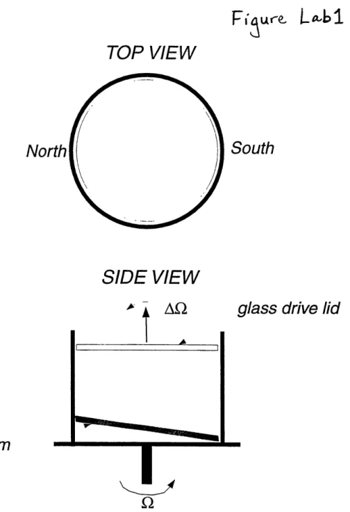
case there are two recirculations, which meet at a hyperbolic point. (see Figure Il a & b) I produce these recirculations in a 'sliced cylinder' rotating tank similar to the original model introduced by Pedlosky & Greenspan (1967). A schematic of the apparatus is shown in figure Lab 1. In this section I will briefly discuss the sliced-cylinder apparatus and the general flow regimes in the tank. I will then outline the particular procedures I employed in my data collection.
Sliced-Cylinder Apparatus:
The tank is placed on a rotating table that is spun counterclockwise at .2=2 (rad/s). The tank is 42.5 cm in diameter and is fitted with a sloping bottom and a submerged 'lid' that is differentially rotated (at a rate AQ) in order to create a 'surface' stress on the
homogeneous fluid. The resulting flow is a single layer on a topographic beta plane forced by uniform upwelling or downwelling (due to the surface stress of the lid). The mean fluid depth is H=20 cm with a total change in depth AH=6 cm. The resulting bottom slope s=O. 15, combined with the standard rotation rate for these experiments produces a topographic beta, / = fs/H = 3(ms)f. For the remainder of this work I adopt northern
-hemisphere terminology in referring to the shallow (poleward) end of the tank as 'north', and the deeper end as 'south'. In addition, in discussing the velocity field below I utilize and coordinate system with +x to the east and +y to the north. I generally ignore any motion in the +/-z direction, as the flow is assumed to be horizontal except in the frictional boundary layers.
The transparent, rotating lid fits within the circumference of the tank, supported by a ring that sits on the top edge of the tank (the top view of the tank is left open for
imaging). I control the rate of rotation of the lid through a computer interface system and a stepping motor. (Please see Appendix A for the details on this motor control system). In these experiments the lid is always rotated in the clockwise (anticyclonic) direction. This
EK WEK = A 2
EK
where v=.01 (cm / s- 1)
is the kinematic viscosity of water, the working fluid, and the lid rotation range from .0076<A.Q<.2777 (rad/s), (with the majority of experiments performed in the range: .0173<A2<.048 (rad/s)). Further details on these and other dimensional and non-dimensional values for the tank are given in Table Lab 1.
With the topographic beta and surface stress, a number of different flow regimes are conceivable. In all of these experiments the bottom slope is held constant and the lid rotation rate is variable. At low to moderate lid rotation rates, the interior the flow is close to the Sverdrup solution as the change in potential vorticity due to the Ekman downwelling is balanced by vortex columns stretching as they move 'south' across the sloped bottom. This balance is confirmed by the small value of Us / PEL2 = 0(2 x 10⁻⁴).
A return flow must balance this southward flow in the interior, and this occurs in a narrow boundary current along the western wall of the tank. On the scale of the boundary current, the surface forcing is unimportant and the structure of current depends on the primary physical factor balancing the change in topographic beta: inertia, bottom friction, or lateral friction. In this case the effects of lateral friction (which would give a Munk
boundary layer solution) and bottom friction (likewise a Stommel boundary layer) are comparable, but S, (at 0.7 cm) is larger than 6s (at 0.5 cm). Therefore the Munk solution best describes the flow in the tank at low inertial values. At higher inertial values (i.e. with stronger lid forcing) the primary balance is between the topographic beta and inertia so the western boundary becomes more jet-like. Here the boundary layer thickness' are defined as (Pedlosky, 1987):
where rek = 3Ef / D is the inverse of the spin-down time determined by the Ekman bottom layer and is equal to .0014 (1/s) in this tank. Us is the interior Sverdrup velocity. Again,
please see Table Lab 1 with the dimensional values for this tank. Many previous
investigators have explored aspects of similar experimental flows. Since my goal in this investigation is to compare two specific flow configurations, I refer readers to previous work for detailed description of the flow regimes in a sliced-cylinder tank. (Pedlosky & Greenspan (1967), Beardsley (1969, 1975(11)), Beardsley and Robbins(1975), Pedlosky,
etal. (1997) and Griffiths & Kiss (1999)). Griffiths and Kiss (1999) present an excellent account of the mechanical and technical details in this type of set-up.
As the lid forcing is increased the flow speeds up and the inertial terms in the equations of motion become more important than the frictional terms. In our present notation, this means that 6, 2 8 . The highly inertial boundary current shoots up the western edge of the tank, separates from the wall, and forms a wave-like pattern across the
northern section of the tank. (see Figure U 1 c-f which is described in the next section) At 6, /,m = 1.10 a set of closed streamlines arises in the tank south of the first large meander in the inertial jet. This 'inertial' recirculation forms north of the 'Munk' recirculation.
For a small window of lid forcing, (1.10 < S1 / ,m < 1.40) both of these
recirculations: the 'inertial' and the 'Munk' exist simultaneously (see Figure Ul). In cases with uniform lid forcing (i.e. the closest we get to steady flow) a unique hyperbolic point exists between these two recirculations, and it is exactly this feature of the flow I
investigate. The balance between the Munk and inertial boundary layer thickness' determines whether the single or double recirculation configuration exists, so I use the value 3 = 6, / M to describe the forcing. This parameter is easily computed as, with the
above parameter settings we find, 8 = 6, / b, = 8.1(A.Q/ Q)A
In order to investigate the flow in the region of a hyperbolic point in an unsteady case, I sometimes force the lid in an unsteady fashion (so that the lid rotation rate oscillates
slightly around an average value). The lid rotation rate is then:
AQunsteadv = AQ(1 + A,,s, sin(2t / Ti,>))
where A is the average or 'background' lid rotation rate, A,,., is the amplitude of oscillation, and T,, is the period of the oscillation. Most of the unsteady runs are at
A,,c =0.05, although a few are at values up to A,,c =0.15. The period of oscillation is
always set equal to the time it takes the lid to complete one full rotation because there is some slight unsteadiness at that period due to imperfections in the glass lid. Therefore
T, = T,,, and is usually on the order of a few minutes.
Data Collection Procedure:
The Pulnix camera is attached to a frame rotating with the table so that images are stationary with respect to the tank. In the resulting images we are looking down on the tank and only the lid and particles and/or dye appear to be moving. I used neutrally buoyant particles in the tank for two purposes : first I created 'trajectory' diagram which give a
general qualitative image of the flow and then I calculated the velocity field in order to quantify the time dependence in the tank. I also injected neutrally buoyant dye into the flow. Images of the dye were used for qualitative description of the flow and in calculating the effective diffusivity.
I encountered some amount of trouble with lighting the images well, both getting enough desired light and blocking out background light. Ideally, all light comes from sources rotating with the tank, so that no outside light biases the images as the tank spins.
For the particles runs I wanted to see only the laser light in the final images. I used a 6W Argon ion laser to supply light for the particles runs. The laser itself was water-cooled and sat away from the rotating table. A fiber-optic cable carried the laser beam onto the table via a coupling. Once on the table a specialized lens generated a horizontal sheet of light which shone through tank about 5 cm below the lid.
For the dye runs, I found the images were cleanest when the tank was lit from below. I therefore positioned two 20W fluorescent light bulbs facing upward below the tank. For all experiments I utilized black-out cloths suspended from the ceiling and pinned around the tank to cut down as much as possible on background light. Unwanted light did not pose a significant problem for the dye runs. Some unsteadiness in the lighting (due to both the laser and background light) may have affected the velocity calculations from the particles runs. (I return to this point in describing the velocity data in section VI).
In order to match the density of the particles to the density of the liquid in the tank I used Pliolite plastic particles p = 1.024 (kg/m') and salt water from a seawater intake
p = 1.022 (kg/m') filtered at 50gtm. These particles are hand ground with a mortar and
pestle and then sorted into size classes using a series of sieves. I chose particles of (diameter) d > 250.pm for the runs leading to trajectory diagrams and particles of
(diameter) 150ym d 250gm for the runs used for PIV analysis.
For the particle runs the lab routine was as follows. First I pumped the seawater into the tank. I then prepared whichever particles were necessary and added them to the tank water. The number of particles in the flow varied between runs, the 'trajectory'
diagrams looked better with a fairly low density while the PIV routine clearly worked better with a very high particle density. The next step was to arrange the laser lighting, camera focus, and black-out cloths (as noted above). The VCR or Mv-1000 digital
imaging software was set to record images from the camera. Just before spinning up the tank, the lid rotation was started.
I allowed 12 minutes spin-up time for all of my experimental runs. This time was based on empirical evidence gathered from the general nature of the 'trajectory' diagrams of the flow. Unsteadiness in the flow associated with the spin-up process were not seen after about 7 or 8 minutes (the time for the fastest topographic Rossby wave to cross the tank is 32 seconds and the calculated spin-up time associated with the Ekman bottom layer (1/rek)
is 70 seconds); twelve minutes allowed a generous margin of error. Once spin-up was completed I recorded images.
The trajectory diagrams were created by adding together a series of snapshots taken over some period of time (this process is described below in section VI). In order to calculate the velocity field I utilized a method known particle image velocimetry (PIV). This process finds the velocity field implied by the difference in particle locations between two snapshots taken in close succession (again, see section VI).
In addition to observing the motion of neutrally buoyant particles, I also injected neutrally buoyant dye into the flow. The dye for these experiments is McCormick red food coloring p = 1.02391(kg / m'). In order to create a neutrally buoyant dye [relative to pond water in tank p = 1.022 (kg/m3 ) ], I mixed this dye with pond water and fresh water, in the
approximate ratio: dye:pond:fresh = 50:40:10. This mixture sat in a reservoir (on the rotating table) and was pumped through tygon tubing and into the feed needle by a variable flow, peristaltic pump. I found the pump worked best if I primed the entire injection system before filling the tank. This Variable Flow Mini Pump fed the dye flow through a section of tubing: 1/50" I.D. at a rotor rpm - 0.5. This results in a calculated flow rate of approximately 6 x 10- 3(cm
/s),
which would result in a total input of 8 cm3 over the courseof each run.
The dye was injected for twenty-three minutes in each case used for effective
diffusivity calculations. This time was equal to a single 'winding' time for the slowest case (r=2.5 cm & = 8, / 8,= 1.00) so that the dye line formed a closed circuit before being shut off (For more details on effective diffusivity see section VIII). To show the development of exchange lobes in the tank I simply captured images while the dye was still being
injected. (for details see section VII). In terms of specific procedure, I simply followed the routine outlined above, skipping the addition of particles, using bottom lighting rather than the laser, and beginning the dye injection after 12 minutes of spin-up.
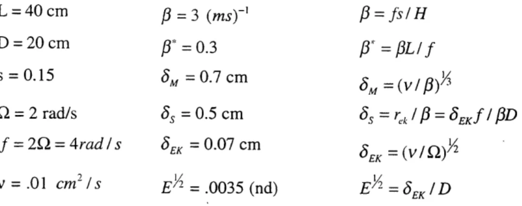
Table Lab 1: Constant Dimensional and Non-Dimensional values for sliced-cylinder lab tank: / = 3 (ms)-' p13= 0.3 8M = 0.7 cm
13=
Js/H X = LIf Q = 2 rad/s f = 2Q = 4rad / s v =.01 cm 2 / s 3s = 0.5 cm SEK = 0.07 cm EI2 = .0035 (nd) (S = r / = 5EKf / PD EK =(v/ )A EK = EK /IDTable: Lab2 Variable Dimensional and Non-Dimensional values for sliced-cylinder lab tank:
A92 (1/s) AGi = (nd) 5 L= 8.1 35m (nd) wEK = -AK2 3EK (cm/s) Us = wEK / S (crn/s) Uwb = us. L/ 5,,, (cm/s) US / L2 Re = UL/v (nd) Ro = Us / JfL (nd) Ro = AQ/ 22 (nd) SE (nd) .0076 .0038 0.50 .00053 .0035 .047 7.3 x 10-' 14 .0173 .0087 0.75 .00120 .008 .107 1.7 x 10⁻⁴ ,0480 .0240 1.25 .00336 .022 .293 4.6 x 10⁻⁴ 2.2 x 10- 5 5.0 x 10- 5 1.4 x 10⁻⁴ .0019 1.08 .0044 2.47 .012 6.86 L = 40 cm D =20 cm s = 0.15 .2777 .0139 3.00 .0194 N/A N/A N/A 516 N/A .070 39.71
TOP
VIEW
SIDE VIEW
glass drive lid
sloping bottom
Figure Lab 1: Schematic of 'sliced-cylinder' rotating tank apparatus. The entire tank
system rotates at 9 =2 rad/s, while a differentially rotating glass lid spins at AQ, exerting a (variable) surface stress on the fluid. The false bottom is sloped to invoke a topographic beta effect. The resulting flow mimics a subtropical ocean basin with the shallow end of the tank analogous to the poleward or 'North' direction and the deep end representing the equatorward or 'South' direction.
10u