Cardy embedding of random planar maps and a KPZ formula for mated trees

Cardy embedding of random planar maps and

a KPZ formula for mated trees

by

Nina Holden

Submitted to the Department of Mathematics

in partial fulfillment of the requirements for the degree of

Doctor of Philosophy

at the

MASSACHUSETTS INSTITUTE OF TECHNOLOGY

June 2018

@

Massachusetts Institute of Technology 2018. All rights reserved.

Author ...

...

Signature redacted

Department of Mathematics

May 4, 2018

C ertified by ...

...

Accepted by ...

Signature redacted

Scott Sheffield

Leighton Family Professor of Mathematics

Thesis Supervisor

Signature redacted

N

-'Wi

liam P. Minicozzi II

Department Committee on Graduate Theses

Chairman,

MASSACHUSETTS INSTITUTE

OF TECHNOLOGY

MAY

3

0

2018]

Cardy embedding of random planar maps and

a KPZ formula for mated trees

by

Nina Holden

Submitted to the Department of Mathematics on May 4, 2018, in partial fulfillment of the

requirements for the degree of Doctor of Philosophy

Abstract

The Schramm-Loewner evolution (SLE) is a random fractal curve which describes the scaling limit of interfaces in a wide range of statistical physics models. Liouville quantum gravity (LQG) is a random fractal surface which arises as the scaling limit of discrete surfaces known as random planar maps (RPM).

First, we study Hausdorff dimensions for SLE curves. We prove a KPZ-type formula which relates the Hausdorff dimension of an arbitrary subset of an SLE curve to the Hausdorff dimension of a time set for a two-dimensional correlated Brownian motion. Using our formula, we obtain new and simple proofs for a number of SLE Hausdorff dimensions, and we prove an explicit formula which says how much the Hausdorff dimension of a deterministic set increases upon being conformally mapped to an SLE curve. This is joint work with Gwynne and Miller.

Then we introduce a mating-of-trees construction of SLE in Euclidean geometry in collaboration with Sun. This is the Euclidean counterpart to the mating-of-trees construction of SLE in an LQG environment by Duplantier, Miller, and Sheffield, which plays an essential role throughout the thesis. Finally, we prove scaling limit results for uniformly sampled RPM known as triangulations. In a joint work with Bernardi and Sun we show that a number of observables associated with critical site percolation on the triangulation converge jointly in law to the associated observables of SLE₆ on an independent

V8/3-LQG

surface. In a joint work with Sun we use this and other results to prove convergence of the triangulation under a discrete conformal embedding which we call the Cardy embedding. The conformally embedded triangulation induces an area measure and a metric on the complex plane, and we show that this measure and metric converge jointly in the scaling limit to an instance of the

V8/3-LQG

disk (equivalently, to an instance of the conformally embedded Brownian disk).

Thesis Supervisor: Scott Sheffield

Acknowledgments

Thanks to my advisor Scott Sheffield for his mentorship, advise, and support, and for generously sharing his many ideas and insights. His creativity and enthusiasm is inspiring, and has lead to an interesting research area which I am grateful for the chance to work in.

During my PhD I have collaborated with several people: Stephane Benoist, Olivier Bernardi, Christian Borgs, Jennifer Chayes, Henry Cohn, Christophe Garban, Lisa Hartung, Tom Hutchcroft, Ewain Gwynne, Greg Lawler, Xinyi Li, Russ Lyons, Jason Miller, Serban Nagu, Robin Pemantle, Yuval Peres, Tom Salisbury, Avelio Sepulveda, Scott Sheffield, Xin Sun, Omer Tamuz, and Alex Zhai. Thanks to each of you for the ideas and time you have contributed. Our collaborations have not only been the best way to get acquainted with a wide range of topics in math; it has also made the work on my PhD much more enjoyable.

The mathematics department at MIT has provided wonderful surroundings for the completion of this thesis. There are too many individuals to mention in person, both among professors, fellow graduate students, staff, and instructors. I am thankful for being part of such a stimulating and friendly environment.

I would like to thank Christian Borgs, Jennifer Chayes, Yuval Peres, and Wendelin Werner for their help and advise with the job search process, and Stephane Benoist and Alexei Borodin for agreeing to be on my thesis committee.

I was supported by the Norwegian Research Council for three years of my PhD. I am grateful for this support, particularly since it made it possible to spend half a year at the Newton Institute in Cambridge, UK.

Finally, a special thanks to my family, my close friends, and Georgy for all their support, and for giving me some breaks from research over the past years.

Contents

1 Introduction

1.1 Schramm-Loewner evolutions and Liouville quantum gravity. 1.2 Hausdorff dimensions for SLE and the KPZ formula . . . . 1.3 SLE as a mating of trees in Euclidean geometry . . . . 1.4 Scaling limit results for uniform triangulations to LQG . . . . . 2 An almost sure KPZ relation for SLE and Brownian motion

2.1 Introduction . . . . 2.2 Exam ples . . . . 2.3 SLE and GFF estimates . . . . 2.4 Intersection of the thick points of a GFF with a Borel set . . . 2.5 Proof of Theorem 2.1.1 .

2.6 Multiple points of space-f 2.7 Open questions . . . . .

. . . .

Rling SLE . . . .

. . . . 3 Dimension transformation formula for conformal

an SLE curve

3.1 Introduction . . . . 3.2 P roofs . . . . 3.3 Open questions . . . . 4 SLE as a mating of trees in Euclidean geometry

4.1 Introduction . . . . 4.2 Imaginary geometry and space-filling SLE . . . . . 4.3 Convergence of discrete contour function for , = 8 4.4 Existence and properties of the contour functions

4.5 4.6

maps into the complement of 9 10 14 16 16 23 23 33 41 56 61 65 78 81 81 87 94 97 97 102 105 . . . 108 The SLE is measurable with respect to the pair of contour functions

Proof of Proposition 4.5.5 and Lemma 4.5.7 . . . .

. . . 114 . . . 119 5 Percolation on triangulations: a bijective path to Liouville quantum gravity

5.1 Introduction . . . . 5.2 A bijection between Kreweras walks and percolated triangulations . . . . 5.3 Discrete dictionary I: Spine-looptree decomposition . . . . 5.4 Discrete dictionary II: Exploration tree . . . . 5.5 Discrete dictionary III: Percolation interfaces and pivotal points . . . . 5.6 Continuum mating of trees . . . . 5.7 Convergence to CLE6 on V8/3-LQG . . . .

5.8 Proofs of the bijective correspondences . . . .

7 125 125 131 142 149 158 163 169 175

.

.

.

. . . . . . . . . . . .

5.9 Proofs of the scaling limit results . . . 193

6 Convergence of uniform triangulations under the Cardy embedding 215 6.1 Introduction . . . 215

6.2 Prelim inaries . . . 219

6.3 Proof of the main theorems . . . 223

6.4 The scaling limit of critical percolation . . . 227

6.5 Liouville dynamical percolation through lattice approximation . . . 231

6.6 Liouville dynamical percolation through random triangulations . . . 241

Chapter 1

Introduction

Many random discrete models show particular (random or deterministic) characteristic behavior when the size of the model grows. Often we can define a notion of convergence for the model when its size goes to infinity, and we say that the model has a scaling limit. The limiting object is typically a random continuum object with certain properties that characterize the large-size behavior of the discrete model. A classical example of a scaling limit is Brownian motion, which arises as the limit of random walks. Scaling limits exhibiting the following two properties are of particular interest in this thesis (see Figure 1-1):

" conformal invariance, i.e., the law of the limiting object is invariant under conformal transfor-. mations, and

" universality, i.e., a wide range of discrete models converge to the same limiting object, and the convergence result is not too sensitive to the details of the discrete dynamics.

This thesis studies three such objects and relationships between them: " the random curves known as Schramm-Loewner evolutions (SLE), " the random surfaces known as Liouville quantum gravity (LQG), and e the random distribution known as the Gaussian free field (GFF).

Beside their role as scaling limits for a wide range of discrete models in physics, probability, and geometry, these objects are of interest since one can argue that

combinatorics, they represent 0 0 * 0 0 0 0 0 0 0 0 0 * 0

Figure 1-1: Conformal invariance and universality for Brownian motion. Left: A simple random walk on Z2 and its image under a conformal transformation both converge to Brownian motion in the scaling limit. Figure from S. Smirnov. Right: Random walk on a wide range of graphs (here, a Voronoi tesselation) converge to Brownian motion in the scaling limit.

particularly canonical or natural probability measures on the space of non-crossing curves, the space of surfaces, and the space of distributions (generalized functions), respectively.

In the remainder of this introduction we first give a brief introduction to these objects. Then we give a brief summary of the results in the remainder of the thesis. First we present our results on SLE curves, and then we present scaling limit results for certain discrete surfaces known as random planar maps to LQG.

1.1

_{Schramm-Loewner evolutions and Liouville quantum gravity}

We start by giving a brief introduction to two universal random objects with conformal symmetries: Schramm-Loewner evolutions (SLE) and Liouville quantum gravity (LQG). Then we introduce the

mating-of-trees construction of SLE and LQG. This construction plays an important role throughout

the thesis, and illustrates a natural interplay between SLE and LQG.

1.1.1 Schramm-Loewner evolutions

The Schramm-Loewner evolution is a family of random fractal curves indexed by a parameter , > 0. SLE curves were first introduced by 0. Schramm [SchOO] as a candidate for the scaling limit of the loop-erased random walk (LERW) and the peano curve of the uniform spanning tree (UST). Later they have been proved to arise as the scaling limit of interfaces in a variety of statistical mechanics models, including the LERW for , = 2 [LSWO4a, LV16], percolation for K = 6 [Smi0l], the contour lines of the GFF and the harmonic explorer for r, = 4 [SS09, SS05], the Ising/FK-Ising model for , = 3,16/3 [CS12, CDCH+14, KS16], and the UST for r, = 8 [LSWO4a]. It is also conjectured to describe the scaling limit of the self-avoiding walk for , = 8/3 [LSWO4b].

Schramm-Loewner evolutions can be characterized as the unique family of non-self-crossing curves satisfying two natural properties: conformal invariance and domain Markov property. 0. Schramm [SchOO] proved that there is a one-parameter family of curves satisfying these two axioms, by showing that the driving function of the so-called Loewner evolution associated with the curves must be a constant multiple K of a standard Brownian motion.

Properties of SLEK depend strongly on the value of r,, and SLEK has the following three phases: For r, E [0, 4], SLEK is a simple curve. For , E (4,8), SLE, is a curve which hits its past and the

domain boundary infinitely often, but whose trace has zero Lebesgue measure. For , > 8, SLEK is space-filling, i.e., every single point of the domain is hit by the curve. More recently there has also been constructed a space-filling variant of SLE, for r, E (4,8) [MS17]. This curve is closely related to regular SLEK, and plays an important role in large parts of this thesis. See Figures 1-2 and 1-3 for illustrations.

n(7) (0) 77(o)

E (0,4] K E (4,8) , > 8

Figure 1-2: The phases of SLE (schematic drawing).

The introduction of SLE revolutionized the understanding of several important statistical mechanics models and their scaling limits. Using a relationship between SLE6 and Brownian motion,

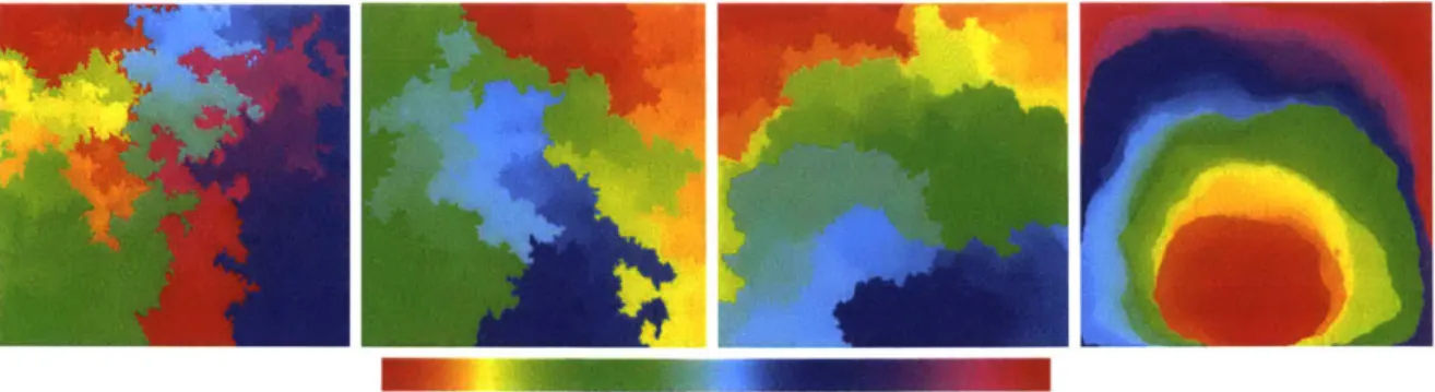
Figure 1-3: Space-filling SLE, in the unit square for , = 6,8,16, 128 (increasing n from left to right). The

color indicates the order in which the points of the square are visited by the curve. Simulations by J. Miller

and S. Sheffield.

the intersection exponents for Brownian motion were rigorously derived [LSW01a, LSW01b, LSW02c,

LSWO2a], confirming conjectures from the physics literature [DK88, Dup98] and Mandelbrot's

conjecture [Man82] that the Hausdorff dimension of the frontier of a planar Brownian motion equals 4/3. Exponents for critical percolation on the triangular lattice were derived in [SW01, LSWO2b],

also confirming conjectures from the physics literature. Furthermore, as we will see later in this thesis, the introduction of SLE has greatly improved the understanding of LQG.

We refer to [Wer04, Law05, BN16] for further background on the SLE.

1.1.2 Liouville quantum gravity

The Gaussian free field (GFF) [She07] is a random distribution [DS11, MS16c, MS17]. Given a

simply connected domain D C C the zero boundary GFF h is the standard Gaussian on the Hilbert

space closure Hl(D) of Co (D) for the Dirichlet inner product (f, g)v := fD Vf - Vg dx dy. In other words, if

#1,

02,... is an orthonormal basis for Co (D) and Oz, O2, ... are i.i.d. standard Gaussians, we can define h formally by h =

Zl

aj#$. This infinite sum does not converge in the space of functions, but it does converge in the space of distributions, and an instance h of the GFF is almost surely an element in the Sobolev space H-(D) for any E > 0. One can also define the GFF with

free boundary conditions and the whole-plane GFF. These distributions are defined modulo a global

additive constant, since (f, g)v = (f + c, g)v for any constant c E R and any functions

f,

g E Hl (D)

or f, g E H1(C). The GFF is conformally invariant, i.e., if

#

: D' -+ D is a conformal map and h is GFF on D, then h o

#

has the law of a GFF on D'. The Gaussian free field may be viewed as a generalization of a standard Brownian motion to two time dimensions (and still one space dimension). Furthermore, one can argue that it represents a natural random perturbation of a harmonic function, since the Hamiltonian used to define the discrete GFF is minimized for harmonic

functions. The GFF arises as a scaling limit in a wide variety of settings [Ken01, RV07, BG15, JLS14].

The setting of primary interest in this thesis is the one of random planar maps (see the end of this

subsection).

Given -y E (0, 2) and with h a GFF or a related kind of field, '-Liouville quantum gravity (y-LQG) can be formally defined as the random Riemannian manifold with metric e-h(dX2 + dy2).

Since h is a distribution and not a function, this definition does not make literal sense. However,

one can prove [DS 11, RV14] that the area measure eyh dx dy associated with this metric can be rigorously defined by considering regularized versions of the field. If hE is a regularized version of h with regularization parameter e > 0, then e-h: dx dy defines an area measure on C. For many natural definitions of h, this area measure can be proved to converge as E -+ 0, such that the limiting

area measure is independent of the exact definition of hE.

The GFF can also be used to define LQG measures supported on certain other subsets of

C [DS11, Berl7]. For example, it induces a natural length measure along SLEK type curves for r E (0, 8), and the free boundary GFF induces a length measure along OD. Later in this thesis we also define an LQG measure supported on the so-called pivotal points associated with an instance of the conformal loop ensemble CLE6 [She09], which is the loop version of SLE6.

Miller and Sheffield [MS15b, MS16a, MS16b] proved in a series of works that for y = 85/3, a -- LQG surface can also be equipped with a natural metric or distance function. They proved that the resulting metric space is equivalent to an instance of the Brownian map. See Section 1.4 for further details.

Figure 1-4: The discrete Gaussian free field on (22)

n

[0, 1]2 for n 20 (left) and n 100 (right). The discrete GFF converges to the continuum GFF in the scaling limit. Simulations by J. Miller and S. Sheffield.

I I"

Figure 1-5: Left and middle:

y-LQG

for -y 1, 1.5, 1.75 (increasing -y from left to right). The simulations have been made such that each of the squares in the figure contains approximately the same -LQG area, e.g., the large gray squares represent regions where the GFF is rather small. Right: A metric ball on a 85/3-LQG

surface (equivalently, on an instance of the Brownian map conformally embedded into the complex plane). The colors indicate the distance to the midpoint of the square, and the black region contains the points in the complement of the metric ball. Simulations by J. Miller and S. Sheffield.

A planar map is a proper embedding of a connected planar graph in the 2-dimensional sphere,

considered up to deformation (i.e., orientation preserving homeomorphism). A triangulation is a planar map where all faces have three edges. See Figure 1-6. The study of planar maps goes back to Tutte [Tut68], who worked on enumerating planar maps in the context of the four color theorem. Mullin [Mul671 worked on enumerating planar maps with a distinguished spanning tree. In the physics literature random maps have been extensively studied using random matrix techniques and as a model for random geometry [BIPZ78, DFGZJ95]. For algebraic and geometric motivations for the study of planar maps see e.g. [LZO4].

Figure 1-6: Triangulations with sphere topology, disk topology, and whole-plane topology, respectively. A triangulation of a disk is a planar map where all faces have three edges, except for a distinguished face with arbitrary degree and simple boundary.

4

I

,# (

Figure 1-7: Random planar maps in three universality classes which converge to y-LQG in the scaling limit. We see that the distortion of the Euclidean sphere is larger for large y. Left: Bipolar-oriented map,

y

4/3 1.15. Middle: FK-weighted map, q = 0.5 and -y

a

1.24. Right: Uniformly sampled map, -y =,8/3 1.63. Simulations by J. Bettinelli.

The set of planar maps may be equipped with several natural probability measures. For example, from a certain class of planar maps (e.g. triangulations, quadrangulations, or simple maps) with a given number of vertices, one may choose a map uniformly at random. In the physics literature it is also common to sample a planar map such that the probability of sampling a particular map is proportional to the partition function of some statistical physics model on the map. For example, one may consider the Ising model, an FK model, or the uniform spanning tree.

Random planar maps (RPM) sampled from several of these probability measures converge (or are conjectured to converge) to -- LQG in the scaling limit. Uniformly chosen random planar maps correspond to -y = /3. When discussing convergence of random planar maps one may consider a variety of different topologies. We will discuss some of these in Section 1.4. The surfaces which typically arise in these scaling limit results are variants of -- LQG known as the -y-LQG sphere, the -y-LQG disk, and the -- LQG plane, respectively, depending on the topology of the discrete surface.

1.1.3 The peanosphere and mating of trees

The peanosphere is the random object we obtain when considering a pair (q, h), where

" q is a space-filling SLE, in C starting and ending at oc, " h is the field on C associated with the -y-LQG cone with y2

(0) = 0

Figure 1-8: The boundary length process for a space-filling SLE,, on top of an independent -y-LQG surface

for -y2_{ir = 16 has the law of a correlated two-dimensional Brownian motion Z = (L, R).}

and q and h are independent. The peanosphere was first introduced by Duplantier, Miller, and Sheffield [DMS14]. They proved that an instance of the peanosphere is encoded by a correlated planar Brownian motion Z = (Li, Rt)tc-, _{in the sense that an instance of Z and an instance of} (,q, h) can be coupled together so they generate the same

a-algebra.

Given (r, h), we obtain Z by studying the boundary length process for q parametrized by -- LQG mass. More precisely, for any t - R, Lt (resp. Rt) is the LQG length of the left (resp. right) frontier of 'q((-oo, t]), relative to the length of the frontier at time 0. The correlation between the coordinates of Z is - cos((y27r)/4)

[DMS14, GHMS17]. See Figure 1-8 for an illustration.

The peanosphere Brownian motions L and R each encode an instance of an infinite-volume continuum random tree [Ald9la, Ald9lb, Ald93]. The peanosphere may be interpreted as a welding or gluing of these two trees. It is therefore often referred to as the mating-of-trees construction of

SLE and LQG. See Figure 4-3.

The peanosphere provides a powerful tool for studying SLE and LQG, and it has recently been used to prove a number of new properties of SLE, LQG, and the associated discrete models

[MS15b, MS16a, MS16b, GHS18a, GM17b, GM17a, GM16, GHS17, GMS17] (see additional references

in the discussion of the peanosphere topology in Section 1.4). The peanosphere allows to prove properties of SLE and LQG using properties of Brownian motion, and it provides a natural framework for proving scaling limit results for discrete models. We will see an example of the former application of the peanosphere in the first part of the thesis, and an example of the latter application of the peanosphere in the third part of the thesis, and in the second part of the thesis we will study a variant of the mating-of-trees construction in a Euclidean environment.

1.2

_{Hausdorff dimensions for SLE and the KPZ formula}

Since the introduction of SLE 20 years ago there have been multiple works studying the fractal properties of SLE by computing the Hausdorff dimension of the curve or of related sets [ABV16,

AS08, Bef08, GMS18b, JVL12, MSW14, MW17, MWW15, NW11, RS05, SSW09, WW15]. This has

improved the understanding of the associated discrete models, due to the close relationship between exponents for rare events in statistical physics models and Hausdorff dimensions for SLE.

Many dimensions and exponents calculated rigorously by mathematicians using SLE were first conjectured in the physics literature. One famous example of this is the Brownian intersection exponents (see the introduction of Chapter 2 for further background and references). One commonly used method in the physics literature for such calculations is the KPZ formula. The KPZ formula [KPZ88] is a non-rigorous and explicit formula which relates exponents for statistical physics models on random planar maps to the corresponding exponents for the model on a Euclidean lattice. In some cases the calculation of the exponent is much easier on the random planar map.

In recent years several versions of the KPZ formula have been established rigorously. In Theorem 2.1.1 we prove a new rigorous version of the KPZ formula in the framework of the peanosphere. Observe that on the peanosphere any subset X c C may be associated with a time set X :=

-1(X)

for 77. Equivalently, X is a time set for the correlated planar Brownian motion Z = (L, R) which describes the evolution of the boundary lengths. We prove the following explicit formula, which relates the a.s. Hausdorff dimension dimw(X) of X to the a.s. Hausdorff dimension dimwj(X) of X, under the assumption that X is independent of the -- LQG surface

2 2

dim((X) = 2 +

)

dim(Z) dimH(Z)2

2 2

We interpret dimn(X) as the -- LQG dimension of X. See Figure 1-9.

'(I)

X = r(X) C C

XcR

Figure 1-9: We interpret the Brownian motion dimension dim-(X) in the KPZ formula (1.1) as the y-LQG dimension of X

c C. This interpretation is natural, since any cover of

X by intervals I c R provides a cover of X (and vice versa), and the length of I equals the -y-LQG mass of the associated subset 71(I) of C.

Our formula is directly useful for computations, since the LQG dimension is explicitly given as a Brownian motion dimension. In many cases the Brownian motion dimension is easier to calculate than the SLE dimension. We give several examples of this in Sections 2.2 and 2.6 by giving new and very short proofs for the dimension of several SLE sets of interest, including the trace of the SLE curve, SLE double points, SLE cut points, and SLE m-tuple points. Our KPZ formula is also interesting since, unlike most of the other KPZ formulas in the math literature, it does not rely on the underlying Euclidean geometry.

In Theorem 3.1.3 we use the KPZ formula (1.1) and the one-dimensional KPZ formula of Rhodes and Vargas [RV1 1] to describe how the dimension of a set Y C R changes upon being mapped to an SLE curve by a conformal map. More precisely, if 77 is a chordal SLEK in H for ,?

$

4, Kt c H is the unbounded complementary component of

([0,

t]) for t E

R,

and ft : Kt -+ H is a conformal map which fixes infinity, then the following holds a.s. for any deterministic set Y C R on the event that {f '(Y) c 77}

dim-H fJ-1(Y) = 4), (dim-H Y), (1.2) where 4) is the explicit function given in (3.2). See Figure 1-10 for an illustration, and see Theorem 3.2.1 for a related result.

()dim-H(X) _{dimw (Y)}

X f(Y) _{BM KPZ Id KPZ}

s . dimQ(X) - dimQ(Y)

o

Figure 1-10: Left: Illustration of the dimension transformation formula (1.2). Right: An illustration of the proof of (1.2), where dimQ(-) denotes (some notion of) quantum dimension. Using the Brownian motion KPZ formula (1.1) we relate dimw(X) and the quantum dimension dimQ (X) := dimn (X). Using a one-dimensional KPZ formula we obtain a similar correspondence for Y C R. The quantum dimensions may be related by using invariance of LQG measures under conformal transformations.

1.3

SLE as a mating of trees in Euclidean geometry

In Chapter 4 we introduce the natural mating-of-trees construction of SLE in a Euclidean environment. We consider an instance T of space-filling SLE, n > _{4, in C, parametrized by Lebesgue area measure.} Then we define the Euclidean contour functions Z = (Lt, Rt)tCR to be the continuous processes that describe the evolution of the 1 + 2/r,-Minkowski content of the left and right, respectively, frontier of 77.

We prove that, as in the case of SLE, on a 4/A-dLQG surface, the instance q of space-filling SLEK is determined by the pair of contour functions Z. Therefore 77 may be obtained by mating or gluing of the pair of trees encoded by L and R. Furthermore, we show that the discrete contour functions associated with an instance of the uniform spanning tree on Z2 converge in the scaling limit to Z for K = 8.

1.4

Scaling limit results for uniform triangulations to LQG

Recall from Section 1.1.2 that the discrete surfaces known as random planar maps (RPM) converge to LQG in the scaling limit. When discussing convergence of RPM one may consider at least three different topologies:

" Gromov-Hausdorff topology, i.e., the random planar map converges as a metric space. " Weak topology on measures on C and uniform convergence for metrics (i.e., distance functions)

on C, where the measure and metric associated with a map is obtained by a discrete conformal embedding of the map into a subset of C.

" Peanosphere (or mating-of-trees) topology, which is defined by convergence in law to the peanosphere Brownian motion Z of certain random walks encoding the planar map decorated by a statistical physics model.

We will briefly describe each of these notions of convergence, starting with the Gromov-Hausdorff topology. A planar map defines a metric space if we let the distance between two vertices be proportional to their graph distance. It has been proved by Le Gall [LG13], Miermont [Mie13], and others [BJM14, Abr16, ABA17, BLG13, BMR16, GM17c, CLG14] that certain uniformly sampled planar maps converge in law for the Gromov-Hausdorff distance to the metric space known as the Brownian map (or to related Brownian surfaces). The Brownian map is an abstract metric measure space with the topology of the sphere and has Hausdorff dimension 4. The Brownian disk (resp. plane) is a variant of the Brownian map with disk (resp. whole-plane) topology. Recall from

Section 1.1.2 that an instance of the Brownian map (or the disk or plane variants) is equivalent to 8/3-LQG in the sense that the two surfaces can be coupled together so they determine each other in a natural way. In particular, a 8/3-LQG surface has a metric or distance function. For

y

: V8/3 a -- LQG surface is not known to be equipped with a natural metric, and convergence of

RPM in the associated universality classes for the Gromov-Hausdorff topology has not been proved. A planar map embedded into a subset of the complex plane defines an area measure on C. The area of U C C is proportional to the number of vertices contained in U. It is conjectured (see e.g. [DS11]) that for a large class of embeddings with conformal properties this area measure converges in the scaling limit to the -y-LQG area measure for some -y depending on the universality class of the planar map. See Figure 1-11. In Theorem 6.1.3 we prove the first convergence result of this kind for uniform planar maps, conditional on a series of other works (see also Section 1.4.1).

bijection

(M, P) (Wk) kEZ

convergence measurability

(h, ) (Zt)

Figure 1-11: Two commonly considered notions of convergence for RPM. Left: A uniformly sampled triangulation is embedded into the sphere. Counting measure on the vertices defines an area measure on the sphere, which we prove converges to 8/3-LQG in the scaling limit for the Cardy embedding. Figures by N. Curien. Right: Illustration of peanosphere convergence. A map M with a statistical physics model P is encoded bijectively by a walk W. By the peanosphere construction, an instance (h, 77) of SLE,-decorated 4/#-LQG is equivalent to an instance of a planar Brownian motion Z. The walk W converges to the Brownian excursion Z in the scaling limit, which we interpret as a convergence result of (M, P) to (h, q).

Certain maps decorated with statistical physics models may be encoded bijectively by two-dimensional walks. Often this encoding is a discrete analog of the peanosphere encoding of SLE and LQG. If the walk converges to a correlated Brownian motion Z in the scaling limit, we say that the decorated map converges in the peanosphere topology to the SLE-decorated -- LQG surface associated with Z. See Figure 1-8. The value of , and -y may be determined by calculating the correlation between the coordinates of the random walk [DMS14, GHMS 17]. Convergence results for decorated planar maps in this topology have been established for maps in several universality classes [Shel6b, GMS18a, GS17, GS15, GKMW18, KMSW15, GHS16].

In Chapter 5 we prove a peanosphere convergence result for percolation-decorated triangulations to SLE6-decorated 8/3-LQG. The bijection, which is illustrated in the left part of Figure 1-13, is

based on a ten-year-old bijection by 0. Bernardi [Ber07a]. Furthermore, we strengthen the topology of convergence of the percolation-decorated map by showing convergence of a number of interesting percolation observables. For example, we study the percolation cycles, the percolation exploration tree, and the pivotal points (see Figure 1-14). The scaling limit of the observables can be described in terms of an instance of SLE6 on V8/3-LQG. The observables we study are encoded in a nice way

by the random walk, and we prove the scaling limit result by showing sufficiently strong convergence of the random walk to Brownian motion. The scaling limit of the observables can be described in terms of an SLE6 q on top of an independent V8/3-LQG surface.

17

Figure 1-12: The figure illustrates the idea of three common ways to embed a planar map into a sphere or a subset of the complex plane. Left: We obtain a Riemannian manifold by equipping each face of a triangulation with the standard Euclidean metric. By the uniformization theorem, this manifold may be embedded by a conformal map into either the sphere, the unit disk, or the complex plane. Middle: A circle packing of a planar map associates each vertex with a circle, and two circles are tangent if and only if the corresponding vertices are adjacent. For triangulations of a sphere the circle packing exists and is unique up to M6bius transformations. Figure from J.-F. Le Gall. Right: In the Tutte embedding the coordinates of each interior vertex is the average of the coordinates of the neighboring vertices. Existence and uniqueness of the Tutte embedding holds if we fix the position of the boundary vertices. Our embedding result in Theorem 6.1.3 uses a fourth embedding, which is illustrated in Figure 1-15.

R (M,P) b W a babcbbabccacc z L

Figure 1-13: Left: Bijection between percolation-decorated triangulations and walks with steps a = (1, 0),

b = (0, 1), and c = (-1, -1) that make a cone excursion. Right: By the peanosphere construction, an SLE6-decorated 8/3-LQG surface is equivalent to an instance of a Brownian cone excursion with correlation

1/2. The L (resp. R) coordinate of Z describes the length of the left (resp. right) frontier of r/ or exposed parts of 0D. Compare with the infinite volume case in Figure 1-8.

1.4.1

Convergence of Cardy embedded uniform triangulations

In Chapter 6 we prove convergence to a /8/3-LQG disk (equivalently, to the Brownian disk) of conformally embedded triangulations. We remark that two of the papers [GHS18b,ASW18] which are referred to in the proof are still in preparation. We embed the planar map into an equilateral triangle A using an embedding we call the Cardy embedding, named after Cardy's formula [Car92, Smi0l] for percolation crossing probabilities. The embedding is defined by considering crossing probabilities for percolation on the planar map.

The embedded triangulation defines an area measure on A (the vertex counting measure) and a metric or distance function on A (the graph distance). We show that these quantities converge in the scaling limit to the area measure and distance function, respectively, of a V8/3-LQG disk. Furthermore, if we decorate the triangulation by critical percolation, the percolation cycles will converge to an instance of CLE6 which is independent of the 8/3-LQG surface.

The proof proceeds by proving a quenched scaling limit result for percolation on uniform triangulations to SLE6. See Figure 1-16. Convergence of the Cardy embedding can be deduced

Figure 1-14: Theorem 5.7.4 gives convergence in law of several interesting observables of a uniformly sampled triangulation with percolation. Left (upper): The percolation cycles describe the interface between red and blue clusters. We show joint convergence in law of number of observables of these cycles, e.g. the length of the cycles and the number of vertices enclosed by each cycle. Left (lower): The exploration tree defines an exploration of the faces of the map, such that the branch towards a given face (when possible) has blue (resp. yellow) on its left (resp. right) side. We show convergence of the finite marginals of this tree, where each branch is parametrized such that one edge is crossed in one unit of time. Right and middle: A pivotal point is a vertex such that changing its color makes percolation cycles merge or split. The figure shows four kinds of pivotal points in orange for an instance of percolation on a triangulation. We show convergence of counting measure on the pivotal points.

almost immediately from this convergence result. To our knowledge, our convergence result is the first quenched scaling limit result to SLE6 for critical percolation since Smirnov's famous proof of

conformal invariance of critical site percolation on the triangular lattice [Smi011.

In the remainder of this section we briefly outline the proof of the quenched convergence result, with reference to important results we take as an input. In [GHS18b] we prove joint convergence in metric and peanosphere topology for a uniform triangulation with percolation. The idea of the proof is to iterate the convergence result of [GM17a], where joint convergence is proved for metric topology and a variant of the peanosphere topology for a single (non-space-filling) percolation interface. This implies in particular that if we consider a coupling such that (Ma, Pn) -+ (h, q) and

(Mn, Pn) -+ (h, _{ff) a.s., jointly in metric and peanosphere topology and with Pn and Pn independent,} then h and

h

are associated with the same instance of the Brownian disk.

The above paragraph gives an annealed convergence result to SLE6 for percolation on the planar

map. To obtain a quenched convergence result we need to argue that if we resample the percolation on the planar map, we get an independent SLE6 in the scaling limit. In particular, the curves q

and i considered above are independent. We proceed by proving a mixing result [GHSS18] for continuum Liouville dynamical percolation (LDP), which describes the scaling limit' of dynamical percolation on the planar map. Dynamical percolation on a planar map is a process where the color of the vertices are dynamically updated so we obtain a percolation valued process (Pt)tgo. Liouville dynamical percolation is a dynamically changing instance (qt)tmo of space-filling SLE6 on

a 58/3-LQG surface. The mixing result for continuum LDP is obtained by studying LDP on the triangular lattice and prove that the scaling limit of this process is continuum LDP. Our proofs use

In fact, we do not prove that continuum LDP is the scaling limit of dynamical percolation on the planar map. Instead, we prove that a cut-off version of dynamical percolation converges to a cut-off version of continuum LDP, which is also sufficient.

B

OX

C A

3a (V =IP

a

- C

Figure 1-15: Illustration of the definition of the Cardy embedding. The three marked vertices a, b, c are mapped to the vertices A, B, C, respectively, of the equilateral triangle A. The interior vertex v is mapped to the point x E A, such that certain percolation crossing probabilities for v are (approximately) the same as the CLE6 crossing probabilities for x. More precisely, we consider the probability

ja(v)

that there is a

blue percolation crossing separating a and v from b and c, and the corresponding probability PA(x) in the continuum, in addition to the same probabilities PB(x), PC(x), Pb(v), Pc(v) with the roles of a, b, c permuted.

7- .K w W W 7 *~.I 4-*

~-

-*A-1 4

~

* *-o~-.

*

I

/ .~ >~, Wi

Figure 1-16: S. Smirnov proved that the percolation interface between blue and yellow for critical percolation on the triangular lattice (left) converges to SLE6 in the scaling limit. Theorems 6.1.3 and 6.1.5 prove the

same result in a quenched sense for uniform random triangulations which are Cardy embedded into a subset of the complex plane (right; schematic drawing of the embedding).

Figure 1-17: Discrete and continuum LDP. Left: Dynamical percolation on a triangulation. Each vertex is associated with an independent Poisson clock, and when the clock of a vertex rings its color is flipped. (The vertex changing color is marked in orange.) Observe that the changes to the percolation cycles are small, except when the vertex which changes color is pivotal. The limiting dynamics are completely governed by the color of the pivotal points. Right: Continuum Liouville dynamical percolation. For an instance of CLE6

(equivalently, space-filling SLE6) on top of a /8/3-LQG surface we sample a Poisson point process (PPP) on

the pivotal points, where the intensity of the PPP is given by an LQG measure supported on the pivotal points. When the "color" of a pivotal point is changed, CLE6 loops merge or split. The purpose of the solid

color inside the

loops

is to distinguish between the different loops.

PA(X) = Ii2

4

results on dynamical percolation in [GPS10, GPS13, GPS18] and our study of the Euclidean pivotal measure in [HLLS18, HLS18]. See Chapter 6 and Figure 1-17 for further details.

Chapter 2

An almost sure KPZ relation for SLE

and Brownian motion

The peanosphere construction of Duplantier, Miller, and Sheffield provides a means of representing a -- Liouville quantum gravity (LQG) surface,

y

E (0, 2), decorated with a space-filling form of Schramm's SLE, , = 16/y 2 E (4, oo), q as a gluing of a pair of trees which are encoded by a correlated two-dimensional Brownian motion Z. We prove a KPZ-type formula which relates the Hausdorff dimension of any Borel subset A of the range of q which can be defined as a function of 77

(modulo time parameterization) to the Hausdorff dimension of the corresponding time set q-1(A). This result serves to reduce the problem of computing the Hausdorff dimension of any set associated with an SLE, CLE, or related processes in the interior of a domain to the problem of computing the Hausdorff dimension of a certain set associated with a Brownian motion. For many natural examples, the associated Brownian motion set is well-known. As corollaries, we obtain new proofs of the Hausdorff dimensions of the SLEK curve for r,

$

4; the double points and cut points of SLEK for r, > 4; and the intersection of two flow lines of a Gaussian free field. We obtain the Hausdorff dimension of the set of m-tuple points of space-filling SLEK for r, > 4 and m > 3 by computing the Hausdorff dimension of the so-called (m - 2)-tuple 7r/2-cone times of a correlated planar Brownian motion.

This chapter is based on a joint work with Ewain Gwynne and Jason Miller [GHM15].

2.1

Introduction

2.1.1 Overview

The Schramm-Loewner evolution (SLE,,) [SchOO] and related processes such as SLE,(p) [LSWO3, SW05, MS16c] and the conformal loop ensembles (CLEK) [She09, SW12] have been an active area of research for the past sixteen years. One line of research in this area has been the confirmation of exponents computed non-rigorously by physicists in the context of discrete models from statistical physics. Many of these exponents were derived using the so-called KPZ relation [KPZ88], which is a non-rigorous formula which relates exponents for statistical physics models on random planar maps to the corresponding exponents for the model on a Euclidean lattice, such as Z2. Exponents derived in this way are said to be obtained from "quantum gravity methods." This method of deriving exponents has been very successful because the computation of an exponent in many cases boils down to a counting problem which turns out to be much easier when the underlying lattice is random (i.e., one considers a random planar map). Perhaps the most famous example of this type are the so-called

Brownian intersection exponents, which give the exponent of the probability that k Brownian motions

started on OBE(O) at distance proportional to

e

from each other make it to 1D without any of their traces intersecting. These exponents were derived using quantum gravity methods by Duplantier in [Dup98]. The values of the Brownian intersection exponents were then verified mathematically in one of the early successes of SLE by Lawler, Schramm, and Werner in [LSW01a, LSW01b, LSWO2c]. Following these works, a number of other exponents (hence also Hausdorff dimensions) have been calculated using SLE techniques, many of which were previously predicted in the physics literature

[ABV16, ASO8, Bef08, GMS18b, JVL12, MSW14, MW17, MWW15, NW11, RS05, SSW09, WW15].

Our main result is a rigorous version of the KPZ formula that relates the a.s. Hausdorff dimension of a set associated with space-filling2 SLEK, [MS17], ' E (4, oc), to the a.s. Hausdorff dimension of a certain Brownian motion set in the context of the so-called peanosphere construction of [DMS14], which we review below. This serves to reduce the problem of calculating the Hausdorff dimension of any set associated with SLE, SLEK(p), or CLEr for ,

$

4 in the interior of a domain to the problem of calculating the Hausdorff dimension of a certain (explicitly described) set associated with a correlated two-dimensional Brownian motion. There are numerous formulations of the KPZ formula in the literature, see e.g. the original physics paper [KPZ88], in addition to more recent and

rigorous formulations in e.g. [Arul5, BGRV16, BJRV13, BSO9b, DMS14, DRSV14b, DS11, RV11]. As

explained just above, the KPZ formula is typically applied to compute the Euclidean dimension of fractal sets, after deriving the quantum dimension heuristically or rigorously by quantum gravity techniques. In our formulation the quantum dimension is explicitly given by the dimension of some Brownian motion set, hence our formula is directly useful for computations.

To illustrate the application of our main theorem, we will obtain new proofs of the a.s. Hausdorff dimensions of several sets, including the SLE curve for K : 4, the double points of SLE, the cut points of SLE, and the intersection of two flow lines of a Gaussian free field [Shel6a, MS16c, MS16d, MS16e, MS17]. We will also use our theorem to calculate the a.s. Hausdorff dimension of the m-tuple points of space-filling SLEK,, ' E (4,8), by calculating the Hausdorff dimension of the so-called

(m - 2)-tuple cone times for correlated two-dimensional Brownian motion. The statement and the proof of the dimension result for (m - 2)-tuple cone times do not rely on quantum gravity techniques or results in the remainder of the chapter.

The main motivation of our theorem is to convert SLE dimension questions into Brownian motion dimension questions, since these are often much easier to solve. However, the result also works in the reverse direction. One example of a Brownian motion set whose dimension has not yet been directly computed to our knowledge is the set of times not contained in any left cone interval. Under the peanosphere correspondence, this set corresponds to the CLEK, gasket for ' E (4,8), the Hausdorff dimension of which is computed in [MSW14, SSW09].

In Chapter 3, the main theorem of the present chapter (along with a theorem of Rhodes and Vargas [RV111) will be used to prove the following additional dimension formula for SLEK. If q is an SLEK curve for , E (0, 4), and Y is a deterministic subset of R with Hausdorff dimension d E [0, 1], then it is a.s. the case that

dimW

f1(Y)

= 3 4 + - 16Kd 12 + 3K + (4 + K)2 - 16Kd)

for almost every choice of conformal map

f

from

H

to a complementary connected component of 77

which satisfies f(Y) c 77.

'The Brownian intersection exponents were also derived earlier using a different method by Duplantier and Kwon in [DK88].

2

In order to be consistent with the notation of [MS16c, MS16d, MS16e, MS171, unless explicitly stated otherwise we will assume that K E (0, 4) and ,' = 16/K E (4, oo).

2.1.2

_{Review of Liouville quantum gravity and the peanosphere}

We will now provide a brief review of Liouville quantum gravity and the peanosphere construction which will be necessary to understand our main result below. Suppose that h is an instance of the Gaussian free field (GFF) on a planar domain D and -y E (0, 2). The -y-Liouville quantum gravity (LQG) surface associated with h formally corresponds to the surface with Riemannian metric

e-h(z) (dX 2 + dy2), (2.1)

where z x + iy = (x, y) and dx2

+

dy2 denotes the Euclidean metric on D. This expression does not make literal sense because h takes values in the space of distributions and does not take values at points. The area measure

Ph

associated with (2.1) has been made sense of using a regularization procedure (see e.g., [DS11]), namely by taking eyh(z)dz to be the weak limit as e -+ 0 of Ec2/2yh,(z)dz, where hE(z) is the average of h on the circle

BE(z).

One can similarly define a length measure vh by taking it to be the weak limit as

e

-

0

of O7/4eYhe(z)/2dz. We refer to Pa (resp. vh) as the

quantum area (resp. boundary length) measure associated with h. Quantum boundary lengths are well-defined for piecewise linear segments [DS11], their conformal images, and SLE type curves for

y = 2 [Shel6a]. The metric space structure associated with (2.1) has also been recently constructed

in [MS15a, MS15b, MS16a, MS16b, MS15c] in the special case that -y = 8/_13, in which case it is

isometric to the Brownian map [Miel3, LG13]. It remains an open question to construct the metric space structure for -y ,4 //3.

One of the main sources of significance of LQG is that it has been conjectured that certain forms of LQG decorated with SLE or CLE describe the scaling limit of random planar maps decorated with a statistical physics model after performing a conformal embedding, where different y values arise by considering different discrete models [DS11]. So far, this conjecture has been proven only in the case of the Tutte embedding of the -y-mated-CRT map (a discretized version of the peanosphere) for -y E (0, 2) [GMS17]. However, the convergence of other random planar maps decorated with a statistical physics model to LQG decorated with SLE/CLE has been proved with respect to the peanosphere topology, which we will describe below [Shel6b, DMS14, GMS18a, GS17, GS15, MS15c,

GKMW18, KMSW15, GHS16, LSW17]. See also the works [GM16, GM17a] for scaling limit results

for self-avoiding walk and percolation, respectively, on random planar maps toward SLE-decorated V8/3-LQG with respect to the Gromov-Hausdorff-Prokhorov-uniform topology, a variant of the Gromov-Hausdorff topology for curve-decorated metric measure spaces [GM17c].

If D, D are planar domains, W: D -* D is a conformal map, and

h=ho p1 +Qlogl( p-1 )'J where Q= +

,

(2.2)

-y 2

then ph(A) = pjt(op(A)) for all Borel sets A C D. The boundary length measure is similarly

preserved under such a change of coordinates. A quantum surface is an equivalence class of pairs

(D, h) where two such pairs are said to be equivalent if they are related as in (2.2). We refer to a

representative (D, h) of a quantum surface as an embedding of the quantum surface.

One particular type of quantum surface which will be important in this article is the so-called -- quantum cone. This is an infinite volume surface which is naturally parameterized by C and is marked by two points, called 0 and oc, neighborhoods of which respectively have finite and infinite Ph-mass. We will keep track of the extra marked points by indicating a 'y-quantum cone with the notation (C, h, 0, oo). In Section 2.1.4 below, we will describe a precise method for sampling from the law of h for a particular embedding of a

7-quantum

cone into C. This surface naturally arises, however, in the context of any 'y-LQG surface (D, h) with finite volume as follows. Suppose that

z E D is sampled from Ph. Then the surface one obtains by adding C to h, translating z to 0, and then rescaling so that

Pah

assigns unit mass to D converges as C -+

00

to a -- quantum cone. That is, a -y-quantum cone describes the local behavior of a -y-LQG surface near a typical point chosen from Ph.

As explained in [Shel6a, DMS14], it is very natural to decorate a y-LQG surface with either an SLE, , = -y2 , or an SLEs,, ' = 16/7y2. In the case of a -y-quantum cone (C, h, 0, oo), it is particularly natural to decorate it with the space-filling SLE,' process q' [MS17] where q' is first sampled independently of h (as a curve modulo time parameterization), then reparameterized by quantum area so that Ph (17'([s, t])) = t - s for all s < t, and then normalized so that q'(0) = 0. In this setting, it is shown in [DMS14] that the pair Z = (L, R) which, for a given time t, is equal to

the quantum length of the left and right boundaries of 7', evolves as a correlated two-dimensional Brownian motion. Since these quantum boundary lengths are in fact always infinite, it is natural to normalize Z so that Lo = Ro = 0. By [DMS14, Theorem 9.1] (in the case ' E (4,8]) and [GHMS17, Theorem 1.1] (in the case

s'

> 8), the variances and covariances of L and R are given by

4ir

Var(Lt) =

alti,

Var(Rt) =

alti,

Cov(Lt,Rt) = -acoselt, 0 = , (2.3)

with a a constant depending only on r'.

One of the main results of [DMS14] is that the pair (L, R) almost surely determines the pair consisting of the 7-quantum cone (C, h, 0, oo) and the space-filling SLE., process

i'.

That is, the latter is a measurable function of the former (and it is immediate from the construction that the former is a measurable function of the latter). This is natural in the context of discrete models [Shel6b] which can also be encoded in terms of an analogous such pair and, in fact, the main result of [Shel6b] combined with [DMS14] gives the convergence of FK-decorated random planar maps to CLE decorated LQG with respect to the topology in which two surfaces are close if the aforementioned encoding functions are close. This is the so-called peanosphere topology.

As explained in Figure 2-1, L and R have the interpretation of being the contour functions associated with a pair of infinite trees, and (C, h, 0, oo) and q' have the interpretation of being the embedding of a certain path-decorated surface into C which is generated by gluing together the pair of trees encoded by L, R [DMS14].

We remark that the construction in [DMS14] deals with the setting of infinite volume surfaces. The setting of finite volume surfaces is the focus of [MS15c] and the corresponding convergence result in the finite volume setting is established in [GMS18a, GS17, GS15].

2.1.3 Main result

Our main result is a KPZ formula which allows one to use the representation (L, R) of an SLE decorated quantum cone to compute Hausdorff dimensions for SLE and related processes.

Theorem 2.1.1. Let ' > 4 and y = 4/v'7 . Let (C, h, 0, oo) be a -y-quantum cone and let

i'

be an independent space-filling

SLEs,,

parameterized by -y-quantum mass with respect to h and satisfying

7'(0) = 0. Assume that h has the circle average embedding (see Definition 2.1.6 below). Let X

be a random Borel subset of C such that X is independent from h (e.g. X could be a set which is determined by the curve q' viewed modulo monotone reparameterization). Almost surely, for each Borel set X C R such that q'(X) = X, we have

A space-filling SLEK, encodes an entire imaginary geometry of flow lines, which in turn encodes both SLE, and SLEs,-type paths and a CLEK, (see [MS17] and Section 2.1.4 below). The forthcoming work [MSW17] will show that the imaginary geometry framework also encodes a CLE,. Therefore, Theorem 2.1.1 reduces the computation of the dimension of any set in the interior of a domain associated with SLE, or CLE, for , _{, 4 to computing the dimension of the corresponding set}

associated with the correlated Brownian motion Z. As we will discuss in Section 2.1.4 it is often possible to characterize special sets associated with SLE, and CLE,, as time sets of Z with particular properties. Examples of such sets are

1. SLE, curves for K , 4 [Bef08, RS05],

2. double points of SLEK, for K' > 4 [MW17],

3. cut points of SLE,, for ,' > 4 [MW17],

4. intersection of two GFF flow lines [MW17],

5. m-tuple points of space-filling SLEK, for m > 3 and ' E (4,8), and 6. CLEK, gasket for ' E (4, 8) [MSW14, SSW09].

See Table 2.1 for a summary of these sets and their dimensions. We will use Theorem 2.1.1 to calculate the Hausdorff dimension of the first five of these sets in Sections 2.2 and 2.6. The original proofs relied on rather technical two-point estimates for correlations, while our formula provides alternative proofs. In cases where the Hausdorff dimension of the SLE set is known, Theorem 2.1.1 also gives the dimension of the corresponding Brownian motion set. We will use this direction of Theorem 2.1.1 to calculate the dimension of the Brownian motion time set corresponding to the

CLE., gasket in Section 2.2.

The random set X does not have to be measurable with respect to the space-filling SLEK,. However, Theorem 2.1.1 does not hold without the hypothesis that X is independent from h. For example, suppose we take X to be the

7-thick

points of h (see [HMP10] as well as Section 2.4). The -y-quantum measure Ph is supported on X

[DS11,

Proposition 3.4], so since 7' is parameterized by quantum mass, we have dimh(?7')- 1(X) = 1. On the other hand, it is shown in [HMP10] that dimn X = 2 - y2/2, so (2.4) does not hold for this choice of X.

Theorem 2.1.1 is in agreement with the KPZ formula [KPZ88] if the "quantum dimension" of X is defined to be twice the Hausdorff dimension of the Brownian motion set X.

Remark 2.1.2. Theorem 2.1.1 only applies to sets associated with SLE and CLE in the interior of a domain. In order to calculate the Hausdorff dimension of sets associated with chordal or radial SLE which intersect the boundary one may apply [RV11, Theorem 4.1], which implies the following one-dimensional KPZ formula. Let h be a free boundary GFF in the upper half-plane and let

Vh

be the associated boundary measure. Define the quantum dimension of a set X C [0, oc) to be

dimW(X), X := {vh([0,x]) x X}.

Then it holds a.s. that

2 2

dim (X) = ( + 4 dimW(Z- dim-(Z)2. (2.5)

4

4

(The function ( in the statement of [RV11, Theorem 4.1] can be obtained using the scaling properties of the free boundary GFF and [RV11, Proposition 2.5].) At the end of Section 2.2 we will include a