The characterization of particle clouds using optical imaging techniques

(1)

The Characterization of Particle Clouds using Optical

Imaging Techniques

by Elizabeth J. Bruce B.S. Electrical Engineering University of Washington, 1994

SUBMITTED TO THE DEPARTMENT OF OCEAN ENGINEERING IN PARTIAL FULFILLMENT OF THE

REQUIREMENTS FOR THE DEGREE OF

MASTER OF ENGINEERING IN OCEAN ENGINEERING JOINT PROGRAM IN MARINE ENVIRONMENTAL SYSTEMS

AT THE

MASSACHUSETTS INSTITUTE OF TECHNOLOGY AND THE

WOODS HOLE OCEANOGRAPHIC INSTITUTION JUNE 1998

Signature of Author

ep -artfment of Ocean Engineering May 1998 Certified by

Dr. E. Eric Adams Senior Research Engineer Department of Civil and Environmental Engineering Thesis Advisor Certified by

7)/) ,,

Dr. Judith T. Kildow Associate Professor of Ocean Policy Department of Ocean Engineering Faculty Advisor Certified by

i"

b'V L-i-C6Mchael S. Triantafyllou

Chairman, Joint Committee for Applied Ocean Science and Engineering Accepted by

MASSACHUSETTS INSTITUTE

OF TECHNOLOGY

nr.T 231998

Dr. J. Kim Vandiver Chairman, Department Committee on Graduate Studies

(2)

The Characterization of Particle Clouds using Optical

Imaging Techniques

by

Elizabeth J. Bruce

Submitted to the Department of Ocean Engineering on May 22, 1998 in Partial Fulfillment of the

Requirements for the Degree of

Master of Engineering in Marine Environmental Systems Abstract

Optical imaging techniques can be used to provide a better understanding of the physical properties of particle clouds. The purpose of this thesis is to design, perform and evaluate a set of experiments using optical imaging techniques to characterize parameters such as shape factor and entrainment coefficient which govern the initial descent phase of particle clouds in water. Several different aspects of optical imaging are considered and evaluated such as the illumination, camera, and data acquisition components. A description of the experimental layout and procedure are presented along with a description of the image processing techniques used to analyze the data collected.

Results are presented from a set of experiments conducted with particle sizes ranging from 250 to 980um. A shape factor is used to demonstrate how the cloud's shape changes from approximately spherical to approximately hemispherical over depth. The entrainment coefficient is shown to vary both as a function of depth and particle size diameter. The experimental cloud velocity is compared to the output of a simplified version of the model, STFATE, used to simulate the short term fate of dredged materials in water. This analysis provides a method of evaluating the experimental results and examining the feasibility of using the experimental data to refine the input parameters to the model.

Thesis Advisor Dr. E. Eric Adams Senior Research Engineer

Department of Civil & Environmental Engineering Faculty Advisor Professor Judith T. Kildow

Associate Professor of Ocean Policy Department of Ocean Engineering

(3)

ACKNOWLEDGMENTS

There are many people that I would like to thank for all of their support during this project. Dr. Adams your support and guidance will always be remembered -your help in completing this thesis has been invaluable. Thank you for all the encouragement, patience, and constructive feedback. Professor Kildow, you have provided encouragement and motivation all the way through -thank you so much.

I would like to thank Gordon Ruggaber for working with me throughout this entire project -I could not have done it without you. Thank you for all of the advice and assistance.

Thank you Dr. Fantone for reading my thesis, for advising me on the optics-related aspects of this thesis, and for all of the encouragement. I would also like to acknowledge Optikos Corporation (Cambridge, MA) for the loan of equipment used during this thesis. A huge thank you to Timothy Prestero - for all of your help in reading and editing this thesis. Thank you Scott Socolofsky for your assistance in setting up equipment and running experiments. To my friends, thank you so much for your endless support -you are all truly wonderful.

(4)

LIST OF FIGURES AND TABLES

Table 1. Default Initial Parameters and Conditions for CDMOD Sensitivity Analysis. 17 Figure 1. Sensitivity of cloud radius (left) and cloud velocity (right) predicted by

CDMOD varying Cd between 0.1 and 1.0 in increments of 0.1. ... 18

Figure 2. Sensitivity of cloud radius (left) and cloud velocity (right) predicted by CDMOD varying Cm between 1.0 and 1.5 in increments of 0.1... 18

Figure 3. Sensitivity of cloud radius (left) and cloud velocity (right) predicted by CDMOD varying a between 0.05 and 0.4 in increments of 0.05 ... 19

Figure 4. Sensitivity of cloud radius (left) and cloud velocity (right) predicted by CDMOD varying initial volume between 50 and 350 mL in increments of 50 mL... 19

Figure 5. Sensitivity of cloud radius (left) and cloud velocity (right) predicted by CDMOD varying initial velocity the intermediate velocities are 0.0, 1.0, and 5.0-50.0 cm/sec in increments of 5.0 cm/sec... ... 20

Figure 6. Experimental setup for laboratory tests. Source: Ruggaber, 1997 ... 22

Table 2. Summary of particle size ranges and mean values. ... 24

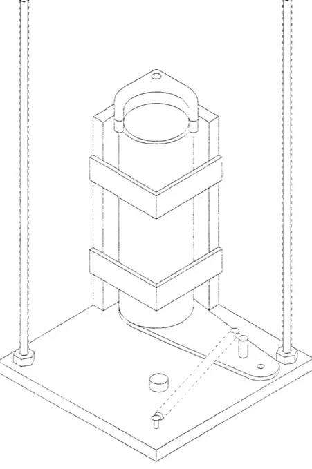
Figure 7. Sediment release mechanism (scale: base is 6" x 6") ... 25

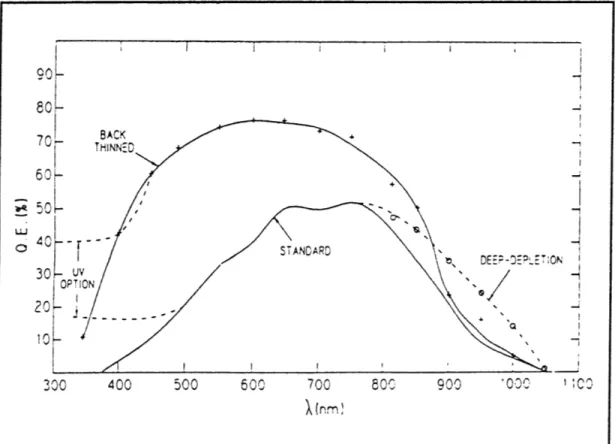
Figure 8. Spectral response of standard CCD detector. Source: Instruments S.A., Inc.27 Table 3. Summary of equipment. ... ... 33

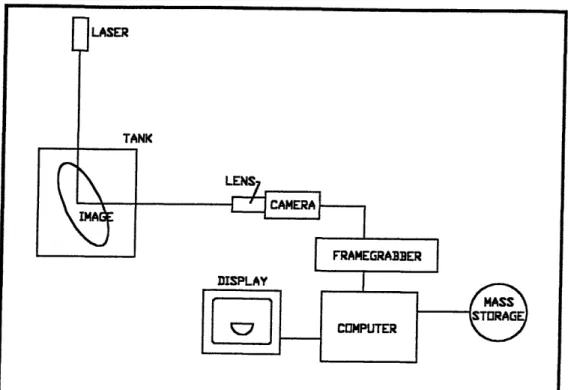
Figure 9. Data acquisition and imaging system layout... 34

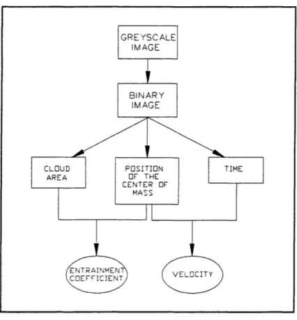
Figure 10. Diagram of data processing routine ... 36

Figure 11. Greyscale image and corresponding binary image for different threshold values. ... 37

Figure 12. Cloud area vs. depth for four particle sizes ... 38

Figure 13. Position of the center of mass vs. time... ... 40

Figure 14. Cloud width vs. depth for four particle sizes... 41

Table 4. Summary of experiments ... 43

Figure 15. Determination of the fall velocity of a spherical particle ... 44

Figure 16. Cloud images of particle size 980um during mid-descent ... 45

Figure 17. Cloud images of particle size 116um during mid-descent ... 46

Figure 18. Images from different stages of the cloud descent for 704um particles... 47

Figure 19. Cloud shape factor, where nr/4 is spherical and nr/8 is hemispherical ... 49

Figure 20. Entrainment coefficient vs. depth for the 704um particles ... 50

Figure 21. Cloud radius vs. depth for 980um particles size ... 51

Figure 22. Cloud radius vs. depth for 250um particles size ... 51

Table 5. Average value of the entrainment coefficient for each particle size ... 52

Figure 23. Cloud velocity vs. depth for four different particle sizes. ... 53

Table 6. Initial conditions used as input to CDMOD ... 54

Figure 24. Variations in CDMOD output velocity for different initial velocities. CDMOD output is for values of a varying from 0.05 (right) to 0.40 (left) in 0.05 increm ents. ... 55

(6)

Figure 25. CDMOD output and experimental cloud velocity for 980um particles. CDMOD output is for values of Cd varying from 0.1 (right) to 1.0 (left) in 0.1

increm ents. ... 56 Figure 26. CDMOD output and experimental cloud velocity for 704um particles.

CDMOD output is for values of Cd varying from 0.1 (right) to 1.0 (left) in 0.1

increm ents. ... 57 Figure 27. CDMOD output experimental cloud velocity for 498um particles. CDMOD

output is for values of Cd varying from 0.1 (right) to 1.0 (left) in 0.1 increments.... 58 Figure 28. CDMOD output and experimental cloud velocity for 250um particles.

CDMOD output is for values of Cd varying from 0.1 (right) to 1.0 (left) in 0.1

increm ents. ... 59 Figure 29. CDMOD output and experimental cloud velocity for 980um particles.

CDMOD output is for values of a varying from 0.05 (right) to 0.4 (left) in 0.05 increm ents. ... 61 Table 7. Initial and final cloud numbers for each particle size. ... 62 Figure 30. Reynolds number vs. drag coefficient, for determination of the real world

particle size (Source: Daily and Harleman, Fluid Dynamics). ... 63 Table 8. Real world particle diameters and corresponding depth ranges for an initial

volume of lm3 and 1000m3 scaled from the experimental data ... 64 Figure 31. Differences in image quality of a standard CCD camera and a progressive

(7)

1. INTRODUCTION

As a result of the long-term build-up of contaminated materials in the bottom sediments of

most major harbors, the safe disposal of material dredged from these harbors has become

an increasingly important issue. When disposing of these contaminated sediments in water it is crucial the different characteristics of sediment transport are understood in order to predict the short-term fate of these sediments. With this knowledge, disposal techniques can be evaluated and refined to accommodate particular situations, depending on different sediment characteristics and water properties such as tidal fluctuations and water depth. A better understanding of the transport of different sediment types in water will help in substantially reducing or even eliminating the amount of contaminated sediment lost to the surrounding water column.

Optical imaging techniques can be used to provide a better understanding of the physical properties of particle clouds. The purpose of this thesis is to design, perform and evaluate a set of experiments using optical imaging techniques to characterize certain parameters of the initial descent phase of particle clouds in water. Several different aspects of optical imaging are considered and evaluated such as the illumination, camera, and data

acquisition components. Experiments are performed in the laboratory and the data is analyzed using different image processing techniques. Results are compared to the output of a simplified version of the sediment transport model, STFATE, to evaluate the

experimental results and to examine the feasibility of using the experimental data to refine certain input parameters to the model.

1.1 Overview of the Management of Contaminated Sediment Disposal

Many different types of particulate waste are dumped into our oceans, including: dredged material, sewage sludge, construction debris, and industrial waste products . Dredged

1 Short-Term FATE, a numerical model developed by Johnson and Fong (1995) of the

(8)

materials make up the largest portion of this waste in the United States, with an

approximately constant value of 100 million wet tons per year for the period 1973 to 1986 (Bohlen, 1990). Managing the disposal of dredged material has become an even more important issue today given the increasing levels of contamination stored in the bottom sediment of our harbors.

Dredged material typically consists of sediment with bulk densities ranging from 1.2 to 2.0 g/cm3_{, depending upon the mineral composition, grain size, and deposit age, and upon the} dredging techniques employed. The finer-grained sediment and higher organic-content particles usually have a higher concentration of contamination. (Bohlen, 1990).

Technically, there is no strict definition for the term 'contaminated sediment'. A 1989 report published by the National Research Council (NRC) defined the term as "a sediment that contains chemical concentrations that pose a known or suspected threat to the

environment or human health" (NRC, 1997). Contaminants, which originate from municipal and industrial outfalls, terrestrial run-off, and accidental spills, include: polychlorinated biphenyl's (PCBs), polyaromatic hydrocarbons, pesticides, trace metals and nutrients (Curran, et. al, 1998) Contaminated sediment must often be dealt with during maintenance of a port or shipping channel, requiring the dredging of bottom sediment. It may also become necessary to remove contaminated sediment from a particular area due to environmental concerns resulting from the long-term build-up of contaminants. There are several different techniques used in the management of

contaminated sediment, ranging from placement of the material in designated open-water sites to in-situ chemical treatment (Pederson and Dolin, 1991).

There are several issues that must be addressed in the disposal of contaminated sediment. One of these issues is how and when the contaminated material should be released from a vessel, since the material's placement may be significantly influenced by currents or tidal fluctuations. Another issue involves how the contaminated material will disperse upon reaching the bottom based on the characteristics of the material.

(9)

Most capping has been employed "in-place", a technique involving careful placement of a clean material over the contaminated material without causing relocation or disruption of the original bed. Alternatively, capping has also been employed in conjunction with the construction of a disposal cell in which contaminated sediments are placed prior to capping (NRC, 1997). In either case, caps typically consist of a natural granular material

such as sand. If capping is to be used the engineers and planners must consider how the capping material will be distributed over the top of the contaminated material, and how effective the cap will be over time.

In order to predict how much of the contaminated sediment will be lost to the surrounding waters and how both the sediment and the capping material will disperse upon hitting the bottom, we must better understand the processes that govern the descent of sediment clouds in water. Relatively little work has been done to characterize the short term fate of sediment in shallow waters despite the fact that the consequences of miscalculating the placement dynamics are much more severe.

The Boston Harbor provides a good example of a shallow water disposal site where accurate placement and capping of contaminated sediment will play a critical role in efforts to deepen portions of the Inner Harbor. The main portion of the Boston Harbor and the principal channel are 40 feet deep whereas portions of the Inner Harbor, including the majority of the port terminals, are only 35 feet deep. In order to increase the number of ships that can access the terminals located within the major tributaries of the Boston Harbor, and to reduce time restrictions on shippers entering the Port of Boston, the US Army Corps of Engineers and the Massachusetts Port Authority (Massport) have entered into a project called the Boston Harbor Navigation Improvement Project (BHNIP).

The Boston Harbor Navigation Improvement Project had to consider several different issues, including the determination of the most efficient manner in which to dispose of the

(10)

dredged material and the development of a means of monitoring the disposal and its environmental impacts. Results of tests conducted on sediment and silt from the bottom of Boston Harbor revealed levels of contamination unsuitable for open-water disposal (Final Environmental Impact Report/Statement EPA, 1995). These results were based on bulk chemistry, bioassay and bioaccumulation data. A proposed open-water disposal site, the Mass Bay Disposal Site, was not selected due to the concerns over the feasibility of accurately placing the contaminated sediment and capping materials in deep water

(approximately 100 meters). Environmental impacts were also a factor in the rejection of the proposed site due to concerns over the loss of contaminated sediments in the water column during placement.

After weighing the costs and benefits of several disposal options, the US Army Corps of Engineers and Massport decided that the most feasible method of safe disposal would be to dredge the channel deeper than necessary, remove the underlying clean material, and dispose of the contaminated material in the channel itself i.e., create in-channel disposal cells. The contaminated material would then be capped by approximately three feet of sand. The clean material will be disposed of offshore. The total cost for the in-place capping project in Boston Harbor is approximately $59 million. The estimated cost for disposing of the clean material is $8 per cubic yard, whereas the cost of disposing of the contaminated material is estimated at $32 per cubic yard (personal communications, Tom Fredette, US Army Corps of Engineers). A good understanding of how both dredged material and capping material behave after being released from the water surface is necessary to ensure the success of this project and justify the added expense of capping. Furthermore, it could be argued that a better understanding of such processes could have lead to a more reliable estimate as to the efficacy of placement and capping in open-water sites, potentially making the originally proposed open-water disposal site a feasible option and significantly reducing the overall cost of the project.

(11)

1.2 Thesis Overview

This thesis examines how optical imaging techniques can be used to characterize the transport of sediment in the laboratory. Four main sections are included. The first section

introduces a simplified version of the STFATE model and discusses its governing

equations, including a brief sensitivity analysis of the model. The second section discusses the equipment tested for both the imaging and the data acquisition systems. In addition, this section presents the experimental layout and an overview of the data processing routine and image analysis. The third section shows the experimental results, including examples of the data images and graphs of the derived parameters. This section also includes a comparison of the output of the sediment cloud model with the experimental data. The final section discusses various experimental issues and presents the overall conclusions of this work.

(12)

2. BACKGROUND

The behavior of sediment clouds has been investigated in the past using both experimental techniques and mathematical models. Abdelrhman and Dettmann (1993) used a model to examine the transport of dredged material released from a hopper dredge in deep waters. Like other applications, their sediment cloud model was based on a modification of the model developed originally by Koh and Chang (1973) and presented by Brandsma and Divoky (1976). Johnson (1978) used field data to calibrate this sediment transport model for shallow waters and the Army Corps of Engineer's STFATE (Johnson and Fong, 1995) derives from this model. Li (1997) investigated the descent of particles using a three-dimensional model and compared the model output with experimentally derived values. The descent of sediment clouds in homogenous fluids has been examined experimentally by Nakatsuji et al. (1990), Bihler et al. (1991), and by Rahimipour and Wilkinson (1992). The descent of sediment clouds in a density stratified fluid has been studied by Luketina and Wilkinson (1994). These previous studies have characterized the convective descent of sediment clouds into three separate phases:

a. The InitialAcceleration Phase occurs within the first few seconds of descent. Depending on release conditions, the cloud of particles accelerates rapidly until the

turbulent forces at the edge of the cloud cause the particles to disperse. The density of the cloud is reduced through the rapid entrainment of ambient fluid.

b. The Self-Preserving Thermal Phase occurs when the cloud organizes itself into a three-dimensional, axi-symmetric, vortex structure similar to a vortex ring. The term "thermal" is used to describe the shape of the cloud in this phase. (The term thermal originates from previous research on atmospheric thermals, where the source of buoyancy was heat. In the case of particle descent, the buoyancy is negative and the source of

buoyancy is the particles themselves rather than heat; however, the word thermal is still used.) During the thermal phase the material in the cloud acts like a homogenous dense liquid and the fall velocities of the individual particles within the cloud are much less than

(13)

the velocity of the cloud itself. As the sediment cloud descends in the water column and shear stresses are induced at the fluid boundaries, ambient fluid is drawn into the cloud. This is known as the entrainment process. The parameter that describes this process is the entrainment coefficient, a. The cloud decelerates until it reaches the third phase of

descent.

c. The Dispersive Phase is characterized by the deceleration of the cloud to the point where individual particles settle out of the cloud. If there are particles of different sizes, the faster settling ones move to the front of the cloud. Eventually, all of the particles in the cloud move downward, and the velocity of the cloud is equal to the settling velocity of the individual particles. The size of the cloud continues to increase and the velocity remains constant.

The dynamic collapse of a sediment cloud occurs when the cloud reaches the bottom surface or when a state of neutral buoyancy is reached. Neutral buoyancy occurs only in stratified waters when the descending cloud entrains positively buoyant fluid from upper layers. Laboratory experiments conducted by Richards (1961), reveal that with sufficient depth and stratification, dynamic collapse of a sediment cloud will occur when the cloud reaches neutral buoyancy, at which point the sediment particles will begin to spread horizontally. Since the majority of sediment disposal projects have been conducted in relatively shallow water, the dynamic collapse of sediment clouds within the water column has not been observed in the field. The understanding of such phenomena is important because finer-grained material will be lost to the water column when the point of neutral buoyancy is reached, potentially causing contamination of the surrounding waters. The experiments conducted in this project are limited to a non-stratified environment; future experiments based on this work will utilize salt water to generate a density-stratified environment, allowing the investigation of the effects of different ambient conditions on the depth of dynamic collapse.

(14)

A TRANSPORT MODEL: CDMOD

The descent of dredged material can be simulated in open waters using the numerical computer model Short-Term FATE (STFATE) developed by Johnson and Fong, 1995. This model derives from the original model developed by Koh and Chang (1973) and currently represents the state-of-the-art in the modeling of discrete discharges of dredged material from barges. The model assumes that the dredged material acts like a hemi-spherical shaped cloud of dense liquid composed of discrete solid components acting independently of each other. Individual particle groups will have different settling rates depending on the values input by the user. Thus smaller, fine-grained particles will remain in the cloud during descent whereas larger-sized particles will settle out of the cloud at an earlier stage, when the vertical fall velocity of the particles exceeds that of the cloud itself.

The STFATE model allows the user to select different values for the entrainment

coefficient. Typically this value is based on either experimental results (Scorer, 1957 and Richards, 1961) or empirically-derived values based on the ratio of percent moisture to liquid limit of the dredged material (Bowers and Goldenblatt's, 1978). Because the duration of convective descent will be highly dependent on the value entered for the entrainment coefficient, it is important to estimate this parameter as accurately as possible when attempting to predict at what depth the cloud will collapse.

The purpose of developing a simplified model, CDMOD (Cloud Descent MODel), is to extract the relevant equations from the STFATE model for the purposes of this project. The equations included in CDMOD characterize only the convective descent stage. CDMOD eliminates certain variables from STFATE and reduces the amount of user-interface. CDMOD also makes it easier to vary and control certain parameters, such as the numerical time step, which enable a more detailed analysis of the initial acceleration phase. CDMOD allows the user to generate output data files based on certain key parameters, which facilitate the graphical representation of data via image-processing programs such as MATLAB.

(15)

3.1 Governing Equations

For the purposes of CDMOD, it is assumed that a single particle cloud will form a spherical vortex structure as it descends. This type of structure has a tendency to draw in fluid from behind it, eventually causing the cloud to become hemispherical. The cloud is assumed to be a hemisphere which remains symmetrical during the entire stage of

convective descent. These assumptions are consistent with the assumptions made in the STFATE model. The equations governing the motion of the cloud are based on the conservation of mass, momentum, and buoyancy. The cloud of particles will descend through the fluid based on its initial momentum and the initial buoyancy of the cloud (Brandsma and Divoky, 1976). As the cloud descends it will displace the ambient fluid, experience drag as a result of the surrounding flow field, and entrain a portion of the ambient fluid. Eventually, particles will drop out of the bottom of the cloud.

The CDMOD input parameters are:

>

initial cloud volume (cc)

>

initial cloud density (grams/cc)

>

initial cloud velocity (cm/sec) > entrainment coefficient (a)

>

drag coefficient (Cd)

>

apparent mass coefficient (Cm)

The model output parameters, each described as a function of time, include:

>

depth

>

average cloud velocity (u) > cloud radius (r)

At each time step i, the cloud radius, r, is calculated based on the volume, V, of a hemisphere:

(16)

As the cloud grows and entrains fluid, the volume is found using: Vi= V(i-1) +

r(i-)

* At

where F is the rate of entrained volume per unit time and At is the time step. F is the product of the surface area of the hemispherical front (27r2), the entrainment coefficient, and the velocity:

r(i-l) = 2 * nt * r(i-) 2* * U(i-1)

The average cloud velocity, u, is derived based on the following equation: ui = Mi / Cm *mi

where,

M = momentum m = mass of the cloud

Momentum is defined by the following formula: M = m u * Cm

where,

Cm = apparent mass coefficient. and is found using:

Mi = Mi-1) + AM * At

The change in momentum, AM, is defined by summing all the forces acting on the system:

AM = [ V(i-) * (P(i-a) -Pa) * g ] [ D(i-1) where,

p = mean density of the cloud pa= ambient water density

g = acceleration due to gravity (981 cm/sec2) D = drag force

The drag force in the vertical direction, D, is described by the following equation: D = 0.5 * pa * Cd * r2 * U(i-1)2

where,

(17)

The mass of the cloud, m, is found by accounting for the volume of fluid entrained by the cloud,

mi = m(i-I) + Pa * F(il) * At

Appendix A includes the code for the MATLAB program CDMOD.

The STFATE model and CDMOD both assume that the entrainment coefficient, a,

remains constant for a non-stratified environment. Typical values used for the entrainment coefficient vary from about 0.15 to 0.35 (Bowers and Goldenblatt, 1978). The value of the drag coefficient, Cd, is typically estimated to be around 0.5 and the value of the apparent mass coefficient, Cm, is estimated to be between 1.0 and 1.5 (Brandsma & Divoky, 1976).

3.2 Model Sensitivity Analysis

CDMOD was run with a range of input values to demonstrate how the cloud velocity and radius varied as a function of the entrainment coefficient, drag coefficient, apparent mass coefficient, volume, and velocity. The output cloud velocity and radius is plotted as a function of depth for these different parameters and initial conditions (see Figures 1-5). Table 1 shows the value of the default initial input conditions used in the following model runs.

Table 1. Default Initial Parameters and Conditions for CDMOD Sensitivity Analysis.

Entrainment Coefficient (a) 0.25

Drag Coefficient (Cd) 0.5

Apparent Mass Coefficient (Cm) 1.00

Initial Volume 100 mL

Initial Velocity 10.0 cm/sec

(18)

0 - 20--8 ---100-- --120 0 5 10 15 20 25 30 3 Cloud Radius (cm) -20 -10 0 -120 10 15 20 25 30 31

Cloud Ve cty (cmisec)

Figure 1. Sensitivity of cloud radius (left) and cloud velocity (right) predicted by CDMOD varying Cd

between 0.1 and 1.0 in increments of 0.1.

O - - -0 -20- -20 1.5 1. 60- -80 -40 0 -80 -80---100- -100---120--- - -120---0 5 10 15 20 25 30 35 5 10 15 20 25 30 35 40

Cloud Radius (cm) Cloud Velocity (cm sec)

Figure 2. Sensitivity of cloud radius (left) and cloud velocity (right) predicted by CDMOD varying C.

between 1.0 and 1.5 in increments of 0.1.

(19)

0 5 10 15 20 25 30 35 0 10 20 30 40 50 60 Cloud Radius (cm) Cloud Velocity (cm/ec)

Figure 3. Sensitivity of cloud radius (left) and cloud velocity (right) predicted by CDMOD varying a between 0. 05 and 0. 4 in increments of 0. 05.

Figure 4. Sensitivity of cloud radius (left) and cloud velocity (right) predicted by CDMOD varying initial volume between 50 and 350 mL in increments of 50 mL.

19 OA -50 -100 -150 ph .05 -200 250 20 -350m. -40- - -- - --140 - - - -g ₀ ₅5so ₁₀ 25 15 20 25 30 35 40 Cloud Radius (cm)

d

a

(20)

I 15 2 Cloud Radius (cm)

20 30

Cloud Velocty (cm/sec)

Figure 5. Sensitivity of cloud radius (left) and cloud velocity (right) predicted by CDMOD varying

initial velocity the intermediate velocities are 0. 0, 1.0, and 5.0-50. 0 cm/sec in increments of 5.0 cm/sec.

The CDMOD output shows that both the cloud velocity and radius are relatively sensitive to the entrainment coefficient compared to the other input parameters. The peak cloud velocities vary from a maximum value of 42 cm/sec to about 24 cm/sec for the range of entrainment coefficients (0.1 to 0.5). In comparison, the peak cloud velocities varies from a maximum value of 34.5 cm/sec to 28 cm/sec for the entire range of drag coefficient values (0.1 to 1.0). The peak cloud velocity ranges from 31 cm/sec to approximately 36 cm/sec for the range of apparent mass coefficient values (1.0 to 1.5). The radius does not appear to have any significant dependence on the apparent mass coefficient. The initial volume which, for a constant initial cloud density is proportional to cloud buoyancy, influences both the cloud radius and the velocity, although the impact is not as significant as the entrainment coefficient given the range of input volumes (50 - 350 mL). The initial velocity does not influence the cloud radius and its effect on the velocity over depth is restricted to the first 10 centimeters, beyond which the velocities converge.

This CDMOD output data clearly demonstrates the range of sensitivities to different model input parameters and initial conditions. Based on this output, it is evident that a

further understanding of how to more accurately predict the entrainment coefficient of the cloud during the convective descent stage would be useful in refining the numerical

(21)

EXPERIMENTAL METHODS

In designing a system for optical imaging there are many factors that need to be

considered. The object that is to be imaged must be properly illuminated in order for the camera to detect the object. A light source must be selected that will provide adequate and relatively uniform intensity over the entire region that is to be imaged. The image must then be detected using an appropriate camera along with the associated optics and captured for later processing and analysis.

An imaging system is comprised of several different components depending on the complexity of the system. Each of these components will contribute to defining the characteristics of the system as a whole. For example, the amount of light that reaches the detector will be a function of both the illuminating intensity and the response of the

camera. In designing the imaging system for the experiments performed in this project certain options were considered, experiments were performed in the laboratory, and a final layout was configured. These options and feasibility tests are described below. The final layout does not constitute the most optimum configuration, as the choices were also a function of cost and time. The final layout is the best configuration obtained given the constraints of these two factors.

4.1 Basic Experimental Setup in the Laboratory

The laboratory setup, used in all of the experiments described below, included a tank and several attached dark rooms (see Figure 6). The tank measures approximately 4 x 4 x 8 feet. Dark rooms, attached to each tank wall, were constructed by attaching a heavy black plastic to a wooden frame. These rooms served to block ambient light from entering the tank, thereby maximizing the image contrast seen by the camera and minimizing the amount of interference or noise caused by stray light. A light source was set up in room A, while the camera recorded the images at 90 degrees, in room B. The particle sample was released from a platform set directly above the water surface in the center of the tank.

(22)

Saltwater Tank

Room

Dark Room.

Sroom A Scale

-1 -0.5 0 in

Figure 6. Experimental setup for laboratory tests. Source: Ruggaber, 1997.

Prior to the start of an experiment, the tank was filled with filtered city water. Two filters are attached to the tank inflow, including both a 1 micron mesh filter and a 0.2 micron filter. The typical flow rate was on the order of 25gpm. A 30 micron mesh filter was

room B

Experimental Tank

D

(23)

attached to a square frame (4 ft x 4 ft) and set at the bottom of the tank to capture particles that were released during the experiments. After a set of experiments was complete, the frame could be removed and the particles dried, sieved and sorted for future experiments.

In the initial set of feasibility experiments, several different types of particles were tested including: sand particles of different sizes and glass beads (soda-lime silica). The painted sand particles used in these experiments were coated with synthetic organic colorants manufactured by Day-Glo Color Corporation (Cleveland, OH). The colorants consisted of a magenta toner and a yellow toner which were dissolved in acetone and then mixed into the sand with a mechanical stirrer. Various colors were produced and tested by mixing different ratios of the two toners.

While testing, it was discovered that the painted sand samples leaked excess paint, coloring the water content of the initial sample volume. This colored water created additional clouds of fluorescing material when released into the tank which obscured the sand itself. After several experiments, which are described below in more detail, it was determined that the glass beads provided a superior imaging signal due to their high reflectivity in water (refractive index of the beads: 1.51-1.52). In addition, they did not

clump or release excess undesirable material. Glass beads provide a good particle for basic cloud characterization and they are readily available in pre-sorted size ranges for a reasonable price.

A selection of glass beads, ranging in size from 2.3mm to 0.044mm, was purchased from Dawson-MacDonald Co., Inc (Wilmington, MA). The beads have a density of 2.50g/cc. A summary of the particle size ranges and their geometric mean values are shown below in Table 2. The mean values are used in the remainder of this report to refer to each group of particle size ranges.

(24)

Table 2. Summary ofparticle size ranges and mean values.

Particle Size Range Mean Size

Name (microns) (microns)

A-100 1200-800 980

A 840-590 704

B 590-420 498

D 297-210 250

AE 150-90 116

Initial feasibility experiments utilized a pneumatic pinch valve as the release mechanism for the particles. One of the problems discovered during the feasibility experiments was the difficulty in generating an axi-symmetric 'thermal-like' sediment cloud using this type of release mechanism. Both the sand and sediment tended to cling to the sides of the valve which resulted in a non-uniform "lopsided" cloud. This non-uniform cloud caused problems in precisely defining the initial conditions of the cloud. In addition, it proved to be much more difficult to characterize using digital imaging techniques. A new release mechanism was designed and used in the remainder of the experiments. This release mechanism uses a long cylindrical LexanTM tube, with inner diameter of 4.4cm, as the container for the particles. A rubber gasket was fitted into the bottom of the cylinder to make it water-tight. The plastic tube provides a smooth surface from which the particles are ejected, resulting in less residual clinging. A plastic lever arm, held in place by the tube itself and a clamp, is connected to a spring which quickly moves the lever arm out from under the tube when the clamp is slightly loosened (see Figure 7).

The sediment samples originally released in the feasibility tests were dry. These samples tended to fall out of the release mechanism in a clump which did not disperse at all during the initial part of the descent. To more accurately simulate the release of wet sediment from a barge or scow, and in an attempt to limit the variation in initial conditions caused by the particles forming clumps, wet samples were used in all subsequent experiments. It was also determined, based on these feasibility tests, that the optimal initial sample

(25)

prevented the particles from reaching the sides of the tank walls as the cloud grows in diameter and minimized any boundary affects associated with the surrounding flow field which would cause disruption in the natural descent of the cloud with depth, altering the

clouds characteristics. I, K, I F

x

. . i '1I i

,u

_>

ii!-]I 1 -II --; K. -4 -h~-4

(26)

4.2 Imaging System Considerations.

In putting together an imaging system for the set of experiments conducted in this project, considerations associated with each of the following components were analyzed and some feasibility tests were performed in the laboratory:

>

illumination

>

camera and lens

>

data collection

>

image processing and data storage.

4.2.1 Illumination

In order to test illumination techniques, different light sources were set up in the laboratory and several types of particles were released into the tank and recorded onto videotape using a standard camcorder (Sharp, Model#VL-L63U).

Imaging with an Ultraviolet Source

Initially, the feasibility of using ultraviolet light as a source for stimulating fluorescence of painted sand particles was tested. The advantage of using painted sand particles is that the color of the paint can be used to distinguish the different particle size characteristics. This technique is most useful during experiments when more than one particle size is released

at the same time.

A vertical plane of light through the tank was created based on simple geometric optics. The source was placed at a set distance from the tank within the constraints of the dark room. Two slits (-0.25" thick), created using cardboard sheets, were placed as far apart as possible between the light source and the tank. Two different ultraviolet sources were obtained and tested. The first lamp was a 100 Watt BIB-100P, Built-in-Ballast Ultraviolet Lamp manufactured by Spectronics Corporation. The ultraviolet radiation from this lamp did not penetrate effectively through the tank, since the majority of the ultraviolet light

(27)

was attenuated by the glass walls. As painted sand particles were released into the water we were only able to observe fluorescence from the sand when the particles were

illuminated from the top of the tank, where the glass did not attenuate the light intensity. The second source tested, a 400 Watt ultraviolet lamp, was rented from a local company (Crimson Tech. Cambridge, MA). Again, it was found that the amount of radiation that penetrated through the glass into the water was not sufficient to illuminate the sand particles. The signal recorded by the video camera was also further attenuated due to the fact that CCD arrays, the light sensing devices used in commercial camcorders, typically have a peak response in the red portion of the spectrum; the response is significantly lower in the blue and ultraviolet region (see Figure 8). It was concluded, given our experimental setup, that ultraviolet lamps do not provide enough intensity for characterizing sediment clouds in the laboratory.

70 BA

30 _OPTIONUv

2I

r I

200 400 500 600 700 800 900 '00C', O C'

(28)

Imaging with a Laser Source

Another set of experiments was performed to examine the feasibility of using laser light to illuminate the painted sand particles. A 6 watt argon-ion laser, with output wavelengths of 488nm and 514nm, was used to create a light sheet that extended the entire length of the tank. The laser light was coupled directly into a fiber optic cable. A cylindrical lens was placed at the output of the fiber to expand the light in one plane, thus creating a vertical sheet of light measuring about 0.5" in width. Painted sand particles were released into the tank and the Sony camcorder was used to videotape the experiment. It was visually apparent during observation of the experiment that the amount of light intensity penetrating the walls of the tank was much greater than in the previous experiments with the ultraviolet light. The videotape also revealed a much brighter image, such that it was possible to distinguish individual sand grains in the tank. It was concluded that the argon-ion laser provided sufficient intensity for recording the images of the particle clouds on camera. Note, that the light detected by the camera was primarily scattered light, since the blue-green laser source did not provide energy in the ultraviolet region for stimulating fluorescence of the painted sand.

4.2.2 Camera & Lens

There are several different types of cameras that could be utilized in this particular application, including: standard charge coupled device (CCD) cameras, progressive scan cameras, and digital cameras. All of these cameras are commercially available; however, the price range varies significantly from a standard monochrome CCD camera to a high end digital camera. Each type of camera differs in how the signal is read out and the manner in which the video signal is produced.

Typical consumer video cameras utilize CCD arrays, making standard CCD cameras a relatively low cost option. The CCD imager is comprised of a matrix of solid-state photosensitive elements on a silicon substrate (Inglis, 1993). Each one of the elements is called a pixel. Typical monochrome CCD cameras have a pixel size on the order of 6-12

(29)

microns. Each of these elements accumulates and stores an electric charge that is proportional to the amount of light incident on the surface of each array element. The

charge is then transferred from element to element through the substrate, using a shift register, to the device output. The clocking out of this output signal then generates an analog output signal which can be digitized and stored or saved directly in analog form on videotape. The number of photosensitive elements in the CCD array determines the resolution of the camera. Each row of elements provides the signal for one scanning line and the number of elements in each column determines the horizontal definition (Inglis,

1993). The sensitivity of the CCD camera is a function of the number of elements

contained in the array; as the number of elements in the device increases, the sensitivity is lowered because the charge generated within each pixel is directly proportional to its area.

Most image sensors in CCD cameras are of interline transfer structure, meaning that after the elements are exposed to the incident light, the charge is integrated, and then

transferred to a vertical register adjoining each element. This charge is then shifted out and horizontally transferred out of the register to be read out as the video signal. Each video output frame is comprised of two fields; one field contains the horizontal odd lines and one field contains the horizontal even lines. Each field is scanned at a rate of 60 Hz per field. A complete frame, containing one odd and one even field, is completed at a rate of 30 Hz. Progressive scan cameras are also interline transfer format; however, instead of incorporating two separate fields in each frame, the progressive scan camera scans all lines sequentially from top to bottom at a rate of 60 Hz. This type of format provides higher resolution, on the order of 484 vertical TV lines, whereas a standard CCD camera is typically limited to a vertical resolution on the order of 350 TV lines. The vertical limiting resolution is the number of horizontal lines that can be distinguished in a dimension equal to the picture height. The horizontal limiting resolution is the number of black and white vertical lines that can be distinguished in a dimension equal to the picture height (Inglis,

1993). Monochrome cameras typically have a higher resolution and better signal-to-noise

(30)

time and storage space, and depending on the application, may not yield significantly more information. Monochrome cameras also have increased light sensitivity compared to a color camera of comparable price.

For this project, two monochrome cameras were selected and tested based on

performance and availability considerations. A Burle TC651 premium interline transfer CCD camera was acquired, with a 1/2 inch format CCD imager and a horizontal resolution of 383 TV lines. The output of the camera is NTSC (RS-170 standard

interlaced scanning at 30 frames/sec) which is the North American monochrome standard video format. The number of active picture elements in the imager is 510 H x 492V. A Pulnix TM-6705AN progressive scan camera was also acquired for testing and

comparison. This camera uses a 1/2 inch progressive scan interline transfer CCD imager with a horizontal resolution of 500 TV lines. The number of active picture elements is 648H x 484V. The advantage of using a progressive scan camera is that it scans every line in every field, avoiding the problems of the interlace scanning format, which become more of an issue when trying to capture a sharp image of an object that is moving

relatively rapidly. However, twice the bandwidth is required for progressive scan cameras compared to the output of standard CCD cameras.

A manual wide-angle zoom video lens was used with both of the cameras. The main advantage of using the zoom lens was the variable focus adjust. The lens had a focal length range of 12.5 to 75 mm. The performance of variable focal length lenses is usually lower than fixed focus lenses. However, the advantages of making final minor

adjustments to the focus outweighed any degradation in system performance resulting from use of the zoom video lens.

4.2.3 Data Collection & Storage

In order to capture and display or store the images from a camera, a data acquisition device must be incorporated into the imaging system. The data acquisition device takes

(31)

the output signal from the camera and stores it in a continuous memory array so that the signal can be displayed or saved as an image file. This type of device is typically called a framegrabber. For standard CCD cameras with a video signal out, the framegrabber includes an analog to digital converter (ADC) which converts the output from the camera to a digital signal (standard framegrabbers use 8 bits per pixel). For digital cameras the CCD charge is converted to a digital signal within the camera. The framegrabber has a separate input which bypasses the ADC so that the signal is captured and stored directly from the camera, minimizing the problems associated with transmission of analog video. Typically a software interface is used with the framegrabber which initializes the board and allows the user to collect a specific number of frames at a certain capture rate. Usually it is the computer processing speed that limits frame capture rate.

Framegrabbers are also capable of converting the output analog signal from a VCR to a digital image data file. One technique that was initially considered for the data acquisition was to record the experiments on videotape and then use the framegrabber to capture the images from the videotape. The disadvantage of this technique is that the signal quality from the VCR would be degraded somewhat compared to the signal received directly from the output of the camera. Over time, the quality of the data stored on magnetic tape would also degrade due to the stretching and wear of the tape itself. Initial feasibility experiments were recorded on videotape and a low-end framegrabber board from Data Translation Inc. was used to acquire images from the videotape for processing. The quality of these images was relatively poor. This was attributed to both the VCR and the framegrabber board that was used in capturing the images. The images contained

significant amounts of noise across the entire image. Video noise is generally defined as any unwanted or irrelevant signal unrelated to the source of data being measured, typically random or thermal noise producing "snow" in the image. Frame averaging techniques were used to try and reduce the noise; however, a significant reduction in noise was not possible. Another disadvantage of using the VCR and the Data Translation Framegrabber was the difficulty in accurately timing the data collection. Since the Data Translation software interface did not allow for sequentially timed frame grabbing, it became

(32)

necessary to rely on the VCR timing which was limited to a resolution of one second. This level of accuracy and image quality proved inadequate.

After considering several different framegrabber boards, the MuTech MV- 1000 board was selected on the basis of processing speed, user interface software capabilities, and cost. The framegrabber board was installed in a Compaq 266 MHz PC computer with 288 Mbytes of RAM. Windows NT was installed as the operating system. This system allowed us to capture up to 700 sequential frames at a rate of 30Hz, which equates to a continuous time period of 23 seconds -a long enough time period for all planned experiments. Each image data file was stored in bitmap form, requiring 302 Kbytes per image file. The framegrabber was able to capture at a rate of 30 Hz and save up to 700 data files. The high data collection rates were obtained because the data was stored in system memory during the capture sequence, which saved processing time by not writing the data to the hard drive. The MV-1000 board is capable of capturing images of a rate up to 200 Hz which was more than sufficient for this project.

The amount of data generated in image processing systems can be enormous. With each experiment using up to 700 image files, approximately 200 Mbytes of drive space is required to store the data. CD-Recordable discs, which can store up to 650 Mbytes of data per CD, were used to backup and store the data for future reference. The amount of

data per experiment could be reduced in future experiments by incorporating certain data reduction or compressing techniques prior to storage. Also, the number of files stored could be reduced by capturing the initial portion of the experiment (approximately the first 3 to 5 seconds) at a rate of 30 Hz and then reducing the rate to 5-15 Hz for the remaining portion of the experiment when the descent velocity of the particles in the water is much lower.

(33)

4.2.4 Image Data Processing

Image processing and analysis was performed in MATLAB, using the image processing toolbox. Standard image processing tools include a wide range of operations, including

image display, filtering, image conversions, analysis, and image transformations. Since the output images from the monochrome cameras used in these experiments are greyscale images, MATLAB stores the data as an intensity image in a single matrix. The intensity matrix is comprised of double precision values ranging from 0.0 to 1.0, representing various intensities - such that 0.0 represents black and 1.0 represents white. Each element of the matrix corresponds to a single image pixel. Intensity matrices can then be

converted to binary images, which is a special type of intensity matrix containing only two intensity levels, black (0.0) and white (1.0). The MATLAB toolbox was used to import, display, and analyze the images acquired from the data acquisition system.

4.3 System Layout

A summary of the equipment used to acquire the data processed in this thesis is shown in Table 3, and the final system layout is diagrammed in Figure 9.

Table 3. Summary of equipment.

Illumination Coherent 6 Watt Argon-ion Laser

Camera Burle TC651 CCD camera

Framegrabber MuTech MV-1000 Board

Computer Compaq 266Mhz PC

Acquisition Software MuTech Sequence Software

(34)

Figure 9. Data acquisition and imaging system layout.

4.4 Experimental Procedures

After filling the tank with water, a target was placed in the image plane located in the center of the tank, for adjustment and focusing of the camera and for later calibration of the relationship between image pixels and distance in the image plane. The target

consisted of both a ruler and a standard optical target comprised of alternating white and black lines, used for judging the contrast and resolution of the imaging system. The

(35)

particle release mechanism was adjusted such that the center of the release tube was aligned at the top of the tank with the cross-section of the laser sheet. The target was then

suspended directly below the sediment release mechanism and illuminated by the laser light. The aperture setting, focal length, f#, gamma value, and gain of the camera were adjusted to obtain adequate intensity and optimal focusing of the system. The camera was rotated and mounted to maximize the vertical distance along the tank imaged by the camera. A calibration image frame was then captured using the framegrabber and stored for later analysis.

The glass beads were weighed and mixed with water such that the mixture was just saturated. The mixture of glass beads and water was then released into the tank. The framegrabber was initialized via the control software to collect a specific number of frames, which varied depending on the length of the experiment, at a rate of 30 Hz. As the glass particles were released and the cloud descended through the water, data images were collected and stored as bitmap images in the computer's system memory. After the experiment, images were saved to the hard drive and eventually backed up and stored on CD-ROM.

4.5 Data Processing

A data processing routine was established and programmed in MATLAB, using the image

processing toolbox, for batch processing of the image files generated in these experiments.

All MATLAB programs written for image processing are located in Appendix 1. Figure 10 shows a block diagram outlining the main processing routine described below.

The following steps outline the processing routine performed for each image file:

1. Convert Image from Greyscale to Binary. Each greyscale image file is imported into

(36)

Figure 10. Diagram of data processing routine.

subsequently used in all of the processing routines. In order to convert a greyscale image to a binary image, a threshold level must be selected such that for all pixels with luminance

values less than the threshold level the pixel value is mapped to 0.0 (black), while all other pixels are mapped to 1.0 (white). In this manner, the threshold level ultimately defines the

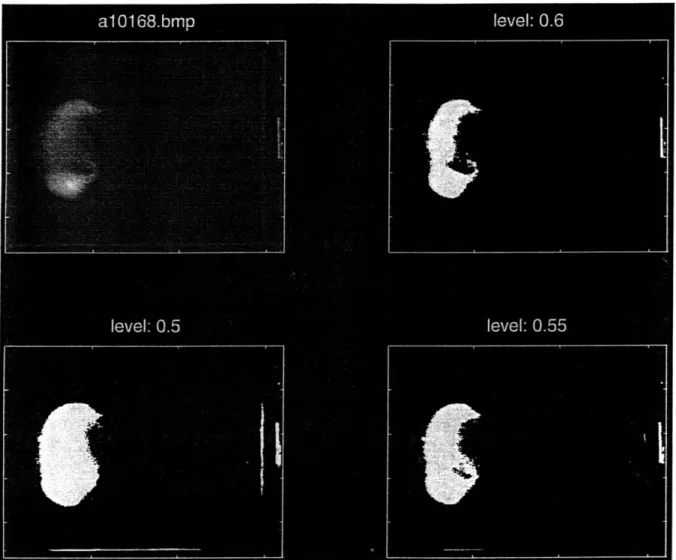
area of the cloud. When the threshold level is selected at higher values, the amount of noise in the resultant binary image is reduced or eliminated. Noise typically includes excess or stray light that appeared in the image due to light reflected into the camera by anything other than the glass particles. Noise also includes light scattered off suspended particles in the water (particles not considered to be included in the cloud) and air bubbles. Reflections off the back walls and edges of the tank, and light reflecting off the bottom edge of the release mechanism are also considered noise. As the threshold value is decreased the amount of noise in the binary image is increased. Figure 11 shows a typical

(37)

Figure 11. Greyscale image and corresponding binary image for different threshold values.

cloud image in greyscale and the resultant binary images using a range of threshold values between zero and one. In processing the images from these experiments, an optimal threshold level was individually selected for each experiment. This was necessary due to the changes in absolute intensity of the image. A significant variation in the initial cloud intensity was due to the variability in how the release mechanism was positioned on the top of the tank with respect to the cross-sectional laser sheet. As a result of these

(38)

variations in intensity, a threshold value was chosen which maximized the sensitivity of cloud detection to account for the entire area of the cloud, and yet minimized the impacts of noise which biased the calculations.

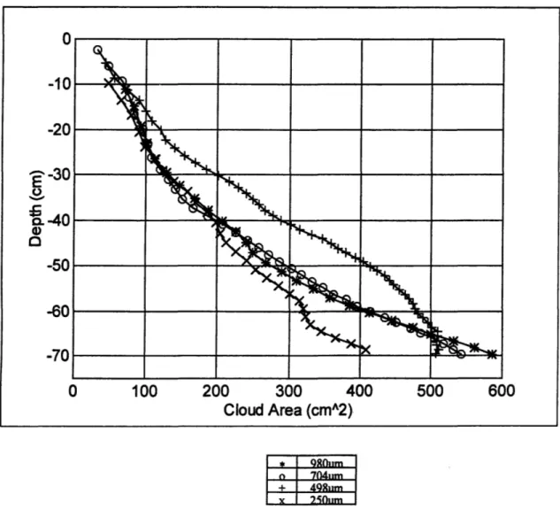
2. Calculate Area of the Cloud. The area of the cloud in the binary image is calculated using a built-in MATLAB routine, bwarea, which estimates the area of the objects in the image using bit quads, 2 x 2 pixel patterns (Pratt, Digital Image Processing, 1991, p.633). Figure 12 shows a plot of cloud area increasing as a function of depth calculated for four of the experiments using different particle sizes.

area vs. dethforfourarti sizes. A 704nm

+ 49Rum

x 750um

(39)

3. Calculate Position of the Center of Mass of Cloud. The position of the center of mass of the cloud in the vertical direction (ybar) is calculated by summing up the total number of pixels with a value of one in the binary image (equivalent to the mass of the cloud in the image), weighted by the index of the pixel's y value and dividing by the total number of pixels with a value of one:

ybar = I(j *BW)/ I BW

where,

ybar position of the center of mass

j value of the pixel's position in the vertical direction

BW value of the pixel's intensity (either 0 or 1 for binary image)

A series of frames captured prior to the release of particles, called blank frames, are used to calculate an average blank value for the position of the center of mass. This value is then used in the following formula to find the position of the cloud's center of mass and eliminate any bias that may be introduced by consistent levels of background noise:

ybarc = ybarf(mf/m) - ybaro (mo/me) where:

mf mass of the image frame mo mass of the blank frame mc mass of the cloud

ybarf position of the center of mass of the image frame ybaro position of the center of mass of the blank frame ybar, position of the center of mass of cloud

Figure 13 shows the position of the cloud's center of mass plotted versus time for four experiments using different particle sizes.

(40)

* 98Mum n 704um + 4M8um

x ?50nm

Figure 13. Position of the center of mass vs. time.

4. Calculate Cloud Width. Next, the maximum diameter, or the nominal cloud width, is determined. The term "width" is used here to prevent confusion with the derived cloud diameter and radius which are calculated based on the cloud area assuming that the cloud is hemispherical. Figure 14 shows how this diameter increases as a function of the position of the center of mass. Note that the cloud width was found by determining, for all values of y, the maximum horizontal distance between pixels with a value of one. It was determined that this calculated width differed on average by only about 0.3 cm from

70 S60 0_S50 -O 0 C 0 20-10 0 1 ₂ 3 4 5 6 Time (seconds)

(41)

the cloud width determined by using the maximum horizontal distance between pixels with a value of 1.0 at the position of the cloud's center of mass. This suggests that the position of the center of mass was located at a point very close to, if not exactly at, the position of the maximum cloud width.

10 15 20 25

Cloud Width (cm)

30 35

n 704unm

+ 49Rum

Figure 14. Cloud width vs. depth for four particle sizes.

5. Calibration. The position of the center of mass, the cloud area, and the cloud width are converted from image pixel values to centimeters by multiplying by the pixel

calibration factor. This factor is determined using the calibration image collected prior to O -10 -20 -30

.

-40 -50 -70

(42)

the start of each set of experiments. The ruler increments in the calibration image were used to calculate the number of image pixels that corresponded to a set distance. The pixel calibration factor is the distance represented by one image pixel. For the set of experiments described in this thesis the pixel calibration factor was determined to be: 0.17 + 0.01 cm. Previous figures have used this pixel calibration factor in converting pixel value to distance in centimeters.

6. Cloud Radius. The cloud radius is derived based on the assumption that the cross

sectional area of the cloud can be approximated as hemispherical (consistent with the assumption made in the STFATE model), thus:

radius = ( (area*2)/ n )1/2

7. Entrainment Coefficient. It is easy to demonstrate that the entrainment coefficient a, defined previously to relate the increase in cloud volume to the cloud velocity, is identical to the cloud spreading rate (increasing in cloud radius with distance). Thus, the

entrainment coefficient of the cloud (a) is calculated using:

a = A radius / Aybar

The entrainment coefficient is also calculated by simply fitting a linear regression to the cloud radius and the position of the center of mass data.

8. Cloud Velocity. The cloud velocity is calculated using the position of the center of mass (ybar) and time increment (time) between each frame, assuming that one frame was

captured every 0.033 seconds:

(43)

5. EXPERIMENTAL RESULTS & ANALYSIS

A summary of the experiments is shown in Table 4, including: the mass of the glass beads, the volume of water used to saturate the beads, and the calculated fall velocity or settling velocity (cos).

Table 4. Summary of experiments.

Mean Particle Initial Initial Particle

Particle Size Dry Water Fall

Size Range Mass Volume Velocity'

(microns) (microns) (grams) (mL) (cm/sec)

1 980 1200-800 100 31 14.4 2 704 840-590 70 20 10.2 3 498 590-420 50 19 6.8 4 250 297-210 40 15 2.9 5 116 150-90 50 19 1.0 1

Fall velocities were calculated based on the mean diameter of each size range.

The fal velocities were calculated based on the following:

>

particles assumed to be spherical

>

diameter = mean diameter of the particle size range

>

specific gravity of particles = 2.5

>

kinematic viscosity = 10-2 cm2/sec

The graph shown in Figure 15 was used to determine the individual fall velocities (class notes for subject 1.67, Professor O. Madsen, MIT, Dept. of Civil and Environmental Engineering).

Although images from Experiment 5 are shown and qualitatively discussed, the analysis presented in this thesis is based on the data collected in Experiments 1-4. This is due to difficulties in Experiment 5 with the release of the smaller particle sizes. Small particles tend to clump upon release into the water, so they were stirred just prior to release. Because it is difficult to predict exactly how the effects of stirring will influence the initial