Optimal Exclusive Perpetual Grid Exploration by Luminous Myopic Opaque Robots with Common Chirality

HAL Id: hal-03130277

https://hal.uca.fr/hal-03130277

Submitted on 3 Feb 2021

HAL is a multi-disciplinary open access

archive for the deposit and dissemination of

sci-entific research documents, whether they are

pub-lished or not. The documents may come from

teaching and research institutions in France or

abroad, or from public or private research centers.

L’archive ouverte pluridisciplinaire HAL, est

destinée au dépôt et à la diffusion de documents

scientifiques de niveau recherche, publiés ou non,

émanant des établissements d’enseignement et de

recherche français ou étrangers, des laboratoires

publics ou privés.

Distributed under a Creative Commons Attribution - NonCommercial - NoDerivatives| 4.0

International License

Optimal Exclusive Perpetual Grid Exploration by

Luminous Myopic Opaque Robots with Common

Chirality

Quentin Bramas, Pascal Lafourcade, Stéphane Devismes

To cite this version:

Quentin Bramas, Pascal Lafourcade, Stéphane Devismes. Optimal Exclusive Perpetual Grid

Ex-ploration by Luminous Myopic Opaque Robots with Common Chirality. International Conference

on Distributed Computing and Networking, 2021, Nara, Japan. �10.1145/1122445.1122456�.

�hal-03130277�

Optimal Exclusive Perpetual Grid Exploration by Luminous

Myopic Opaque Robots with Common Chirality

Quentin Bramas

CNRS, France

Pascal Lafourcade

Aubière, France

Stéphane Devismes

Stephane.Devismes@univ-grenoble-alpes.fr

Université Grenoble Alpes, VERIMAG

ABSTRACT

We consider swarms of luminous myopic opaque robots that run in synchronous Look-Compute-Move cycles. These robots have no global compass, but agree on a common chirality. In this con-text, we propose optimal solutions to the perpetual exploration of a finite grid. Precisely, we investigate optimality in terms of the visibility range, number of robots, and number of colors. In more detail, under the optimal visibility range one, we give an algorithm which is optimal w.r.t. both the number of robots and colors: it uses two robots and three colors. Under visibility two, we design two algorithms: the first one uses three robots with an optimal number of colors (i.e., one), the second one achieves the best trade-off be-tween the number of robots and colors, i.e., it uses two robots and two colors.

KEYWORDS

Luminous myopic robots, perpetual exploration, finite grid, chiral-ity, opacchiral-ity, exclusiveness.

ACM Reference Format:

Quentin Bramas, Pascal Lafourcade, and Stéphane Devismes. 2018. Optimal Exclusive Perpetual Grid Exploration by Luminous Myopic Opaque Robots with Common Chirality. In Woodstock ’18: ACM Symposium on Neural Gaze Detection, June 03–05, 2018, Woodstock, NY . ACM, New York, NY, USA, 12 pages. https://doi.org/10.1145/1122445.1122456

1

INTRODUCTION

We consider swarms of autonomous robots endowed with visibility sensors, motion actuators, and lights of different colors. These so-called luminous robots [16] run in synchronous Look-Compute-Move cycles, where they first sense the environment (Look), then choose a destination and update their light color (Compute), and finally move to the chosen destination (Move).

We deal with luminous robots having very low capabilities. First, they are myopic, i.e., they are only able to sense their surroundings within a limited visibility range. Then, they are opaque. Opacity means that a robot is able to see another robot if and only if no other robot lies in the line segment joining them. Furthermore, they have no global compass, i.e., they agree neither on a North-South, nor a East-West direction. Finally, except from their lights, robots have neither persistent memories nor communication capabilities. This study was partially supported by the French anr projects ANR-16-CE40-0023 (descartes) and ANR-16 CE25-0009-03 (estate).

Woodstock ’18, June 03–05, 2018, Woodstock, NY 2018. ACM ISBN 978-1-4503-XXXX-X/18/06. . . $15.00 https://doi.org/10.1145/1122445.1122456

However, they all agree on a common chirality, i.e., when a robot is located on an axis of symmetry in its surroundings, it is able to distinguish its two sides, one from another.

We are interested in coordinating such weak robots, endowed with both typically small visibility range and few light colors (only a constant number of them), to solve an infinite global task called the perpetual exploration. In this problem, space is partitioned into locations, e.g., rooms in a building, that should be visited by robots. Here, we consider a finite discrete space which is conveniently represented as a graph, where nodes represent locations and edges represent the possibility for a robot to move from one location to another, e.g., through a door or a corridor. In this context, the perpetual exploration requires each node to be visited infinitely often by at least one robot. The direct application of such an exploration is, of course, patrolling in a zoned (maybe hazardous) area.

In this paper, we investigate optimal exclusive solutions to the perpetual exploration of a finite grid, where exclusiveness [1] re-quires any two robots to never simultaneously occupy the same position nor traverse the same edge.

Related Work. The robots we consider are known as luminous robots in the literature. They have been introduced by Peleg [16].

Up to now, exploration tasks have been considered in various topologies, e.g., lines [13], rings [2, 7, 10, 14, 15], trees [12], torus [9], finite [3, 8] and infinite grids [4, 5].

In the context of finite graphs, two main variants, respectively called the terminating and perpetual exploration, have been consid-ered. The terminating exploration requires every possible location to be eventually visited by at least one robot, with the additional constraint that all robots stop moving after task completion. In contrast, the perpetual exploration requires each location to be visited infinitely often by all or a part of robots. Terminating ex-ploration has been tackled in [7–10, 12–14] while [2, 3] deal with the perpetual exploration problem. Notice that Ooshita and Tixeuil consider the two variants of the problem in [15].

In contrast with the present paper, a large part of the literature is devoted to “non-myopic” robots, i.e., robots with an unbounded visibility range, meaning that the snapshot of each robot captures in the whole system configuration; see [2, 3, 8–10, 12–14]. In such a context, robots are always assumed to be anonymous and oblivious, i.e., they have no state and cannot remember the past. Furthermore, opacity and chirality have never been considered in such settings. Exploration algorithms satisfying exclusiveness are proposed in both finite [2, 3] and infinite graphs [4, 5].

However, only few works dedicated to discrete environment, e.g., in (infinite) graphs [4], assume robots have a common chirality. Actually, up to now this property was rather considered in the 2D Euclidean plan; see e.g., [11]. Now, the common chirality has an

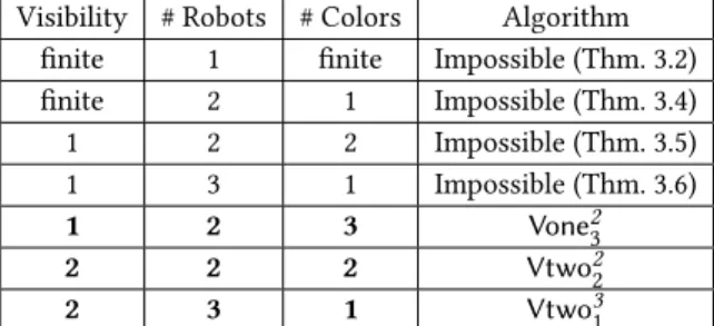
Visibility # Robots # Colors Algorithm finite 1 finite Impossible (Thm. 3.2) finite 2 1 Impossible (Thm. 3.4) 1 2 2 Impossible (Thm. 3.5) 1 3 1 Impossible (Thm. 3.6) 1 2 3 Vone2₃ 2 2 2 Vtwo2₂ 2 3 1 Vtwo3₁

Table 1: Summary of our results.

impact on the number of robots necessary to solve exploration: for example, with visibility range one and few colors (𝑂 (1)), five (resp. six) synchronous robots are necessary and sufficient to ex-plore an infinite grid with (resp. without) the common chirality assumption [4, 5].

To the best of our knowledge, until now exploration with myopic robots was only addressed in finite rings [7, 15] or infinite grid [4, 5]. Hence, the present work is the first study of (perpetual) exploration with myopic (luminous) robots in finite grids.

Contribution. We investigate optimal solutions to the exclusive Perpetual Finite Grid Exploration (PFGE) in synchronous settings using luminous myopic opaque robots. Our contributions are sum-marized in Table 1 and can be split into tight lower bounds and algorithms matching those bounds.

Lower bounds: Under our settings, we establish several lower bou-nds. First, we show in Theorem 3.2 that one robot is not sufficient to solve the PFGE problem, whatever the visibility range is. Then, we prove in Theorem 3.4 that two robots with only one color are not able to solve the PFGE problem, whatever the visibility range is. When the visibility range is one, we demonstrate in Theorem 3.5 that it is impossible to solve the PFGE problem with only two robots and two colors, and in Theorem 3.5 that it is impossible to solve the PFGE problem with only three robots and one color. Notice that all these bounds hold even if exclusiveness is not required. Optimal exclusive algorithms: According to the previous lower

bounds, we propose three optimal algorithms denoted by Vone3₂, Vtwo2₂, and Vtwo1₃, respectively. All these algorithms achieve exclusiveness. Under visibility range one, Vone3₂ solves the PFGE problem using only two robots and three colors. Under visibility range two, Vtwo2₂solves the PFGE problem using two robots and two colors, while Vtwo1₃solves the problem with three oblivious robots (equivalently, three robots with only one color).

Notice also that we explain how to modify our non-oblivious solutions to obtain terminating exploration algorithms, with a con-stant overhead in terms of colors. Finally, we describe a simple transformation to make Vone3₂work in fully asynchronous setting, yet under visibility range two.

Roadmap. Section 2 is devoted to the computational model and definitions. In Section 3, we propose four impossibility results, giving our lower bounds. In Section 4, we describe an algorithm

which is optimal not only w.r.t. the visibility range but the number of robots and colors. In Section 5, we give two solutions for visibility range two, the former uses three robots with an optimal number of colors (one), and the latter achieves the best trade-off between the number of robots (i.e., two) and the number of colors (i.e., two). We conclude with extensions and perspectives in Section 6.

2

MODEL

We consider a set of 𝑛 > 0 robots located on a finite grid made of L ≥ 𝑛 lines and C ≥ 𝑛 columns, i.e., robots evolve in the undirected graph 𝐺 (𝑉 , 𝐸) where 𝑉 = {(𝑖, 𝑗) : 𝑖 ∈ [0, C − 1], 𝑗 ∈ [0, L − 1]} and 𝐸 = {{(𝑖, 𝑗), (𝑘, 𝑙)} : (𝑖, 𝑗) ∈ 𝑉 ∧ (𝑘, 𝑙) ∈ 𝑉 ∧ |𝑖 −𝑘 | + | 𝑗 −𝑙 | = 1}. The size of the grid is then L × C. Grid coordinates are used for the analysis only, i.e., robots cannot access them.

We assume discrete time and at each round, the robots syn-chronously perform a Look-Compute-Move cycle. In the Look phase, a robot gets a snapshot of the subgraph induced by the nodes within distanceΦ ∈ N∗from its position.Φ is called the visibility range of the robots. The snapshot is not oriented in any way as the robots do not agree on a common North. However, it is implicitly ego-centered since the robot that performs a Look phase is located at the center of the subgraph in the obtained snapshot. Then, each robot computes a destination (either Up, Left, Down, Right or Idle) based only on the snapshot it received. Finally, it moves towards its computed destination. We also assume that robots are opaque, i.e., they obstruct the visibility in such way that if three robots are aligned, the two extremities cannot see each other.

We forbid any two robots to occupy the same node simulta-neously. A node is occupied when a robot is located at this node, otherwise it is empty. Robots may have lights with different colors that can be seen by robots within distanceΦ from them. We denote by Cl the set of all possible colors.

The state of a node is either the color of the light of the robot located at this node, if it is occupied, or ⊥ otherwise. In the Look phase, the snapshot includes the state of the nodes (within distance Φ). During the compute phase, a robot may decide to change the color of its light.

In all our algorithms, we also prevent any two robots from traversing the same edge simultaneously. Since we already for-bid them to occupy the same position simultaneously, this means that we additionally prevent robots from swapping their position. Algorithms verifying this property are said to be exclusive. How-ever, to be as general as possible, we do not make this additional assumption in our impossibility results.

Configurations. A configuration 𝐶 in a grid 𝐺 (𝑉 , 𝐸) is a set of pairs (𝑝, 𝑐), where 𝑝 ∈ 𝑉 is an occupied node and 𝑐 ∈ Cl is the color of the robot located at 𝑝. A node 𝑝 is empty if and only if ∀𝑐, (𝑝, 𝑐) ∉ 𝐶. We sometimes just write the set of occupied nodes when the colors are clear from the context.

Views. We denote by 𝐺𝑟the globally oriented view centered at the robot 𝑟 , i.e., the subset of the configuration containing the states of the nodes at distance at mostΦ from 𝑟, translated so that the coordi-nates of 𝑟 is (0, 0). We use this globally oriented view in our analysis to describe the movements of the robots (see, for example, Fig. 1): when we say “the robot moves Up”, it is according to the globally

oriented view. However, since robots do not agree on a common North, they have no access to the globally oriented view. When a robot looks at its surroundings, it instead obtains a snapshot. To model this, we assume that, the local view acquired by a robot 𝑟 in the Look phase is the result of an arbitrary indistinguishable trans-formation on 𝐺𝑟. The set IT of indistinguishable transformations contains the rotations of angle 0 (to have the identity), 𝜋 /2, 𝜋 and 3𝜋 /2, centered at 𝑟 . Moreover, since robots may obstruct visibility, the function that removes the state of a node 𝑢 if there is another robot between 𝑢 and 𝑟 is systematically applied to obtain the local view. Finally, we assume that robots are self-inconsistent, meaning that different transformations may be applied at different rounds. It is important to note that when a robot 𝑟 computes a destination 𝑑, it is relative to its local view 𝑓 (𝐺𝑟), which is the globally oriented view transformed by some 𝑓 ∈ IT . So, the actual movement of the robot in the globally oriented view is 𝑓−1(𝑑). For example, if 𝑑 = Up but the robot sees the grid upside-down (𝑓 is the 𝜋 -rotation), then the robot moves Down = 𝑓−1(Up). In a configuration 𝐶, 𝑉𝐶(𝑖, 𝑗 ) denotes the globally oriented view of a robot located at (𝑖, 𝑗). Algorithm. An algorithm A is a tuple (Cl, Init, 𝑇 ) where Cl is the set of possible colors, Init is a mapping from any considered grid to a non-empty set of initial configurations in that grid, and 𝑇 is the transition function 𝑉 𝑖𝑒𝑤𝑠 → {Idle, Up, Left, Down, Right} × Cl, where 𝑉 𝑖𝑒𝑤𝑠 is the set of local views. When the robots are in Configuration 𝐶, a configuration 𝐶′obtained after one round satisfies: for all ((𝑖, 𝑗), 𝑐) ∈ 𝐶′, there exists a robot in 𝐶 with color 𝑐′∈ Cl and a transformation 𝑓 ∈ IT such that one of the following conditions holds: • ( (𝑖, 𝑗 ), 𝑐′) ∈ 𝐶 and 𝑓−1(𝑇 ( 𝑓 (𝑉𝐶(𝑖, 𝑗 )))) = (Idle, 𝑐), • ( (𝑖 − 1, 𝑗), 𝑐′) ∈ 𝐶 and 𝑓−1(𝑇 ( 𝑓 (𝑉𝐶(𝑖 − 1, 𝑗)))) = (𝑅𝑖𝑔ℎ𝑡, 𝑐), • ( (𝑖 + 1, 𝑗), 𝑐′) ∈ 𝐶 and 𝑓−1(𝑇 ( 𝑓 (𝑉𝐶(𝑖 + 1, 𝑗)))) = (𝐿𝑒 𝑓 𝑡, 𝑐), • ( (𝑖, 𝑗 − 1), 𝑐′) ∈ 𝐶 and 𝑓−1(𝑇 ( 𝑓 (𝑉𝐶(𝑖, 𝑗 − 1)))) = (𝑈 𝑝, 𝑐), or • ( (𝑖, 𝑗 + 1), 𝑐′) ∈ 𝐶 and 𝑓−1(𝑇 ( 𝑓 (𝑉𝐶(𝑖, 𝑗 + 1)))) = (𝐷𝑜𝑤𝑛, 𝑐). We denote by 𝐶 ↦→ 𝐶′the fact that 𝐶′can be reached in one round from 𝐶 (n.b., ↦→ is then a binary relation over configurations). An execution of Algorithm A in a grid 𝐺 is then a sequence (𝐶𝑖)𝑖_∈Nof configurations such that 𝐶0∈ Init (𝐺) and ∀𝑖 ≥ 0, 𝐶𝑖↦→ 𝐶𝑖+1. Perpetual Finite Grid Exploration. An execution (𝐶𝑖)𝑖_∈Nin a grid 𝐺 = (𝑉 , 𝐸) achieves the Perpetual Finite Grid Exploration (PFGE) if for every node 𝑢 ∈ 𝑉 and for every time 𝑡 , there exists a time 𝑡′≥ 𝑡 such that 𝑢 is occupied in 𝐶𝑡′.

An algorithm A that uses 𝑛 robots solves the Perpetual Finite Grid Exploration (PFGE) problem if for every finite grid 𝐺 = (𝑉 , 𝐸) with at least 𝑛 lines and 𝑛 columns and every initial configuration 𝐶₀∈ Init (𝐺), we have every execution of A in 𝐺 starting from 𝐶0 that achieves the PFGE.

Well-defined Algorithms. Recall that robots are assumed to be self-inconsistent. In this context, we say that an algorithm (Cl, Init, 𝑇 ) is well-defined if the global destination computed by a robot does not depend on the applied indistinguishable transformation 𝑓 , i.e., for every globally oriented view 𝑉 , and every transformation 𝑓 ∈ IT , we have 𝑇 (𝑉 ) = 𝑓−1(𝑇 ( 𝑓 (𝑉 ))). All our algorithms are well-defined. However, to be as general as possible, we do not make this assump-tion in our impossibility results. We notice that an execuassump-tion of a

𝑅₁ 𝑅₂ 𝑅₃ R R R B R R R B R R R B

Figure 1: Examples of rules.

well-defined algorithm is uniquely determined by its initial config-uration.

An Algorithm as a Set of Rules. We write an algorithm as a set of rules, where a rule is a triplet (𝑉 , 𝑑, 𝑐) ∈ 𝑉 𝑖𝑒𝑤𝑠 × {Idle, Up, Left, Down, Right} × Cl.

We say that an algorithm (Cl, Init, 𝑇 ) includes the rule (𝑉 , 𝑑, 𝑐), if 𝑇 (𝑉 ) = (𝑑, 𝑐). By extension, the same rule applies to indistin-guishable views, i.e., ∀𝑓 ∈ IT , 𝑇 (𝑓 (𝑉 )) = (𝑓 (𝑑), 𝑐). Consequently, we forbid an algorithm to contain two rules (𝑉 , 𝑑, 𝑐) and (𝑉′, 𝑑′, 𝑐′) such that 𝑉′= 𝑓 (𝑉 )for some 𝑓 ∈ IT . Hence, an algorithm corre-sponds to a set of rules if each destination is the result of applying one of its rules.

As an illustrative example, consider the rule 𝑅1given in Fig. 1. This rule is defined for robots having a visibility range of two. This rule means that, when a blue robot 𝐵 sees three robots with color 𝑅, one on top, one on the left, and one in diagonal, then the blue robot is dictated to move Up. Notice that, due to the opacity of the robots, the state of the topmost node, and the leftmost node, are not accessible. This is indicated by a cross inside the node (to help the reader only). By extension the same rule applied if the view is rotated by 𝜋 , but in that case, the destination would be Down.

In the same figure, rule 𝑅2is a rule where the three black nodes represent a part of the outer boundary of the grid, that we call a wall in the remaining of the paper. Notice that a wall is never hidden behind a robot (due to the opacity) as it simply represents the absence of a node. In our algorithms, we often define similar rules that apply regardless of the presence of a wall in some part of the view. Thus, to avoid defining several time rules with very similar views, we propose a notation to represent several rules in just one picture. For example, rule 𝑅3in Fig. 1 has three nodes hatched with vertical lines, which means that the rule applies regardless of the presence of a wall located at those nodes. In practice, every rule that contains such vertical (resp. horizontal) hatched lines, represents a set of rules obtained by replacing each of those lines either by walls, or by empty nodes. For example, rule 𝑅3in Fig. 1 is a concise representation of rules 𝑅1and 𝑅2.

For a more complex example, refer to the first rule in Fig. 13, which represents a set of 33rules, as there are 3 potential walls (top, right, bottom), and the rule applies whether those walls are at distance 1, 2 or more (i.e., not visible).

Algorithms having locally-defined initial configurations. In a given grid, the set of possible initial configurations of an algo-rithm can be reduced to a singleton. In such a case, the scalability and flexibility of the algorithm is weak. To be more general, we pro-pose algorithms with locally-defined sets of initial configurations.

Configurations in a locally-defined set of initial configurations are defined by colors and relative positions of the robots only. Hence, every two possible initial configurations are equal up to a transla-tion applied to all robot positransla-tions and for a given grid, the set of all possible initial configurations is closed by such translations.

3

IMPOSSIBILITY RESULTS

In this section we prove our four impossibility results; see Table 1 for a summary. Due to the lack of space, several proofs have been moved in the appendix. The technical lemma below is trivial yet very useful since it allows us to consider initial configurations where one robot has an arbitrary position, without the loss of generality. Lemma 3.1. Let A = (Cl, Init, 𝑇 ) be an algorithm that solves the PFGE problem using 𝑛 robots. For every grid 𝐺 with at least 𝑛 lines and 𝑛 columns, for every node 𝑢 in 𝐺, there exist a configuration 𝐶 where a robot is located at 𝑢 and an algorithm A′ = (Cl, Init′, 𝑇) where Init′is identical to Init unless 𝐶 ∈ Init′(𝐺) such that A′solves the PFGE problem using 𝑛 robots.

When there is a single robot that is far enough not to see any wall (using the previous lemma, one can assume that the robot is initially in a center of a large enough grid), then, due to to the self-inconsistency assumption, there exists a possible execution where the robot visits at most two adjacent nodes, hence follows.

Theorem 3.2. The PFGE problem is not solvable with only one robot, for any finite visibility range.

Proof. Assume, by the contradiction, that A solves the PFGE problem with one robot. LetΦ > 0 be the visibility range of the robot. Consider a grid 𝐺 of size greater than (2Φ + 3) × (2Φ + 3). By Lemma 3.1, we can assume, without the loss of generality, that A solves the problem starting from the initial configuration where the unique robot is at a center of 𝐺. Thus, the robot sees no wall. If the algorithm dictates the robot to stay idle, then the robot will stay idle forever, a contradiction. So, the robot moves toward one direction in the globally oriented view, say 𝑑 ∈ {Up, Down, Left, Right}. Now, after the move, the robot is in the same situation: it sees no wall. So, it will again move and the chosen destination in its local view will be the same. However, since the robot is self-inconsistent and the four possible destinations look identical, there is a transformation 𝑓 ∈ IT such that the destination of the robot in the globally oriented view is actually the opposite of 𝑑. Hence, there is a possible execution where the robot starts at a center of the grid and forever alternates between two positions. The perpetual exploration is not achieved in this execution, a contradiction. □ Remark 1. Consider any algorithm solving the PFGE problem with two robots and any configuration where the two robots have the same color and do not see the border of the grid. In this situation, there exist two transformations (e.g., the identity transformation and the 𝜋-rotation), one for each robot, that make their local views identical. In this case and even if the algorithm is not well-defined, whenever one decides to move, the other moves too and the two robots move in opposite direction in the global view, e.g., if one moves Up in the global view, the other moves Down. Conversely, if one stays idle, the other stays idle too. Moreover, if one robot decides to change its color, the other also switches to the same color.

When there are only two robots, the following lemma states that, in many large grids, there exists an execution where the two robots eventually see each other, while one of them is located at a center. This is useful to prove the next two theorems, involving only two robots.

Lemma 3.3. Consider any algorithm A that solves the PFGE prob-lem with two robots and a grid 𝐺 of size at least (4Φ + 6) × (4Φ + 6) whose number of lines or columns is even.

Then, there exists an execution of A in 𝐺 that contains a configu-ration where the two robots see each other and one of them is located at a center of 𝐺.

Proof. We proceed by the contradiction. Remark first that 𝐺 contains at least two centers, 𝑐1and 𝑐2, which are neighbors, by definition. Then, by Lemma 3.1, we can consider, without loss of generality, that A solves the PFGE problem starting from an initial configuration 𝐶 where a robot 𝑟 is located at one of the two centers of 𝐺. Let 𝑟′be the other robot. Now, each time 𝑟 is located at 𝑐1or 𝑐2, 𝑟 does not see any wall by construction of 𝐺 and does not see 𝑟′by the contradiction. So, in such a case if 𝑟 decides to move, all destinations look identical and there is a transformation that makes it move from 𝑐1to 𝑐2if located at 𝑐1, and from 𝑐2to 𝑐1otherwise. Hence, there is a possible execution where 𝑟 visits at most 𝑐1and 𝑐₂and never sees 𝑟′. Consider now such an execution.

Let 𝑢1be a node at distanceΦ + 1 from 𝑐1and distanceΦ + 2 from 𝑐2. By construction of 𝐺, 𝑢1is at distance at leastΦ + 2 from a wall. Moreover, 𝑢1is eventually visited because A solves the PFGE problem. By construction, 𝑢1is necessarily visited first by 𝑟′. Moreover, 𝑟 stays at 𝑐1or 𝑐2and 𝑟′is never in the visibility range of 𝑟meanwhile. When the first visit of 𝑢1by 𝑟′occurs, robots neither see each other nor any wall. Moreover, 𝑢1as a neighboring node, say 𝑢2, at distanceΦ + 1 from a wall, distance Φ + 2 from 𝑐1, and distanceΦ + 3 from 𝑐2. From that point, there exist transformations such that every time 𝑟′decides to move, the applied transformation makes 𝑟′alternatively moves from 𝑢1to 𝑢2, and vice versa, while 𝑟still alternates between 𝑐1and 𝑐2. Hence, from that point, there exists a possible execution suffix where all nodes, except 𝑐1, 𝑐2, 𝑢1, and 𝑢2, are never more visited, a contradiction. □ Theorem 3.4. The PFGE problem is not solvable with two robots and only one color, for any finite visibility range.

Proof. Assume, by the contradiction, that an algorithm A solves the PFGE problem with two robots and one color. Consider a grid of size at least (4Φ+6) × (4Φ+6) whose number of lines or columns is even. By Lemmas 3.1 and 3.3, we can assume, without the loss of generality, that A solves the PFGE problem starting from an initial configuration 𝐶 where a robot 𝑟 is located at a center of the grid and the other is located within distanceΦ from 𝑟. Then, due to the size of the grid (at least (4Φ + 6) × (4Φ + 6)), no robot sees a wall in this initial configuration.

Consider now an execution, starting from 𝐶, where every time the robots see each other without seeing a wall, the applied trans-formations are those that make the local views of the two robots identical. Since initially both robots see each other and one of them is in a center of the grid (i.e., at distance at least 2Φ + 3 from any wall), the other robot is at distance at leastΦ + 3 from any wall.

𝑉₁ 𝑉₂

B

R

R

B

Figure 2: The two views of two robots with colors 𝑅 and 𝐵. Hence, initially their local views are the same and their destinations in the globally oriented view are opposite; see Remark 1 (of course, they cannot stay idle). Thus, in that execution, the middle of the two robots remains constant at least until one robots sees a wall. More formally, if robots respectively have coordinates (𝑥, 𝑦) and (𝑥′, 𝑦′), then the two real numbers 𝑀𝑥 = 𝑥+𝑥

′

2 and 𝑀𝑦 = 𝑦+𝑦′

2 remain constant until at least one robot sees a wall.

Initially, the robot 𝑟 located at a center, say at coordinates (𝑥, 𝑦), is at distance at least 2Φ + 3 from any wall, i.e., 𝑥 ≥ 2Φ + 3 and 𝑦 ≥ 2Φ + 3. The other robot being within distance Φ from 𝑟, so |𝑥 − 𝑥′| ≤Φ and |𝑦 −𝑦′| ≤Φ. Thus, we have 𝑥′≥Φ + 3, 𝑦′≥Φ + 3, 𝑀𝑥 >3₂Φ + 3, and 𝑀𝑦> 3₂Φ + 3.

Consider now the first visited node which is at distanceΦ+2 from a wall. Without loss of generality, assume that one of the closest wall is the left one, i.e., its abscissa is 𝑥 =Φ+2. Since no robot has yet see a wall, we still have 𝑀𝑥 >3

2Φ + 3. By replacing 𝑥 by its current value, we obtain: Φ+2+𝑥₂ ′ > 3

2Φ + 3 ⇔ 𝑥 ′

>2Φ + 4 ⇔ 𝑥′− 𝑥 >Φ + 2. Hence, the two robots neither see each other, nor a wall. From that point, using the same argument as in Theorem 3.2, we can construct a possible execution suffix where each robot either stays idle or alternates between two nodes. Now, in that suffix, there are many nodes that are never visited, a contradiction. □ In the following, we say that a robot is isolated whenever no other robot is within its visibility range.

Theorem 3.5. The PFGE problem is not solvable with two robots, two colors and visibility range one.

Proof. Assume by the contradiction that an algorithm A solves the PFGE problem in this setting. Consider a grid 𝐺 of size at least 10 × 10 whose number of lines or columns is even. By Lemmas 3.1 and 3.3 (recall thatΦ = 1), we can assume, without the loss of generality, that A solves the PFGE problem starting from an initial configuration 𝐶 where a robot 𝑟 is located at a center of the grid and the other is located at the neighboring node. Moreover they have different colors, since otherwise we have a contradiction using the same argument as in the proof of Theorem 3.4. Indeed, the argument remains valid even if robot can change their color because robots with same views modify their color in the same way.

Let’s say that in 𝐶, a robot is blue (𝐵) and the other is red (𝑅). We can choose an execution and the transformations such that, every time a red robot sees a blue robot, its local view is 𝑉1in Fig. 2 and every time a blue robot sees a red robot, its local view is 𝑉2, in Fig. 2. A outputs a single destination 𝑑1, resp. 𝑑2, for the local view 𝑉1, resp. local view 𝑉2. Moreover, in 𝐶, robots initially have local views 𝑉₁and 𝑉2. After one round, robots are either isolated, they have the same color, or their views are 𝑉1and 𝑉2respectively (n.b., the two robots still do not see the border of 𝐺 in this latter case). If robots are

(𝑏)or(𝑐)

(3) (2)

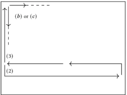
Figure 3: The movement leading to a contradiction.

isolated, we can construct a possible execution where robots remain isolated forever and, depending on the algorithm, they either stay idle or alternate between two positions forever. Hence, in that case, the perpetual exploration is not achieved, a contradiction. If now the robots have the same color after one round, then depending on the algorithm, we can construct an execution where they either stay idle or swap their position forever while maintaining their colors identical, or they become isolated after the second round. In the latter case, they still do not see the border of 𝐺, so we can make the perpetual exploration fails, as previously explained.

Hence, the only remaining case is the one where their views of the two robots are 𝑉1and 𝑉2after the first round. In this case, the movements of robots are periodic while they do not reach a wall. So, either robots alternate between two configurations, or the two robots move in a straight line until at least one robot reaches a wall. In the former case we immediately obtain a contradiction. So, we focus now on the latter case: when a robots reaches a wall, there exists a constant 𝑆 (independent of the size of the grid) such that the two robots can either (1) remain indefinitely in a subgrid of size 𝑆, or (2) remain in a subgrid of size 𝑆 for a finite number of rounds, then leave the wall and move straight toward the opposite wall, or (3) remain at distance at most 𝑆 from the wall until they reach a corner. Fig. 3 illustrates the last two cases. In Case (1), some nodes will not be visited if 𝐺 is large enough, a contradiction. In Case (2), when the robots leave the wall they must be in the same relative positions as initially, rotated by angle 𝜋 (to move to the opposite direction). Indeed, we have just seen that this is the only way the two robots can travel without seeing walls. Hence, when reaching the opposite wall, since they cannot distinguish between the two walls, the robots will perform the same turn, remains in a subgrid of size 𝑆for the same finite number of rounds, then leave the wall to move straight towards the first wall. All the movements are the same as the movement performed when reaching the first wall, but rotated by 𝜋 . Hence, they will end up in the exact same initial position. The two robots will continue this periodic movement infinitely, leaving nodes unvisited if 𝐺 is large enough, a contradiction.

Consider now Case (3). After following the wall (staying at distance at most 𝑆 from it until reaching another wall), the robots reach the corner and again we have three possibilities: either (𝑎) they remain in a subgrid of size at most 𝑆′where 𝑆′is a constant (independent of the size of the grid), (𝑏) they follow a wall (either the same one on the opposite direction, or the new encountered one) for a finite number of rounds, then leave the wall to move in straight line until reaching the opposite wall, or (𝑐) they follow

a wall until reaching another corner. In Case (𝑎), some nodes are never visited if 𝐺 is large enough, a contradiction. In Cases (𝑏) and (𝑐), there exists a constant 𝑆′′(independent of the size of the grid) such that the robots always stay at distance at most 𝑆′′from a wall, and when they reach a new wall, the same thing occurs again, so if 𝐺is large enough, some nodes that are far from all walls are never visited, leading to a contradiction. □ Theorem 3.6. The PFGE problem is not solvable with three robots, one color, and visibility range one.

Sketch of Proof. This theorem is proven by contradiction. As-suming there exists an algorithm solving the PFGE problem in these settings, we first show that, in large enough grids, there is a reach-able configuration where the three robots are far from all walls. We then show that it is possible, within one or two rounds, to make one robot isolated while keeping all robots not seeing any wall (to prove this, there are only few cases to consider, up to rotations, with three robots, one colors, and visibility one). From this latter situation, we show that it is possible to make all robots isolated still while maintaining the walls out of the visibility range of all robots. Being isolated and seeing no wall, robots either stay idle, or there is an execution where each robot alternates between two adjacent nodes while maintaining them isolated and seeing no wall,

a contradiction. □

4

VISIBILITY RANGE ONE: Vone

We present an algorithm, denoted by Vone3₂, which assumes a visibil-ity range one and uses two robots and three colors. By Theorem 3.2, Vone3₂is optimal w.r.t. the number of robots, and by Theorem 3.5, Vone3₂is also optimal w.r.t. the number of colors. An animation illustrating the behavior of Vone3₂is available online; see [6].

Initially, one robot, called the follower, has color 𝐹 and the other robot, called the leader, has any of the two colors 𝐿 and 𝑅. The initial positions of the two robots are arbitrary in the grid, except that they should be neighbors. Hence, the set of all possible initial configurations is locally-defined.

The follower is colored 𝐹 all along the execution, while the light of the leader alternates between color 𝑅 and color 𝐿. Moreover, the two robots always stay neighbors during the execution: we say that they form a group all along the execution. For the purpose of explanation only, we now consider an arbitrary orientation of the grid (n.b., the robots do not know this orientation since they do not agree on a common North): the four walls are respectively at the top, bottom, left, and right in the grid.

For example, consider the initial configuration 𝐶 where (1) the leader has color 𝑅, (2) the group of robots is placed along a line linking the left wall to the right one, and (3) the leader is closer from the left wall than the follower.

From 𝐶, the group first performs an ascending phase: the group moves straight from a wall to another (n.b., from 𝐶, the group first moves toward the left wall), moreover the group moves Up and turns around every time it reaches a wall. Once the group reaches the top wall, it does the same but now moves Down every time it reaches a wall: it switches to a descending phase. So, the group visits all the nodes following a serpentine belt alternating forever between ascending and descending phases.

To achieve these principles, we use the relative positions of the two robots as well as the two colors of the leader to give a kind of direction. Actually, the follower always moves toward the leader without changing its color. In contrast, the leader always moves from its current position to one of its three free neighboring nodes. In some particular cases, the leader uses its color to make the choice. Overall, the leader takes all decisions on the behalf of the group.

For instance, if the robots do not see any wall, the leader moves away from the follower and the follower follows the leader; see the rules in Fig. 4. This makes the group move straight.

F L F R F L F R

Figure 4: Moving straight.

Consider now the case where the leader reaches a wall during an ascending (resp. descending) phase and the leader is not on the line along the top (resp. bottom) wall. Then, the group should turn to reach the immediately upper (resp. lower) line. In this case, the color of the leader is used to decide the rotation sense of the turn. Precisely, a turn is performed in two rounds. Upon reaching the wall, the leader turns Right if it has color 𝑅, Left otherwise (n.b., if the destination line is Up, the phase is ascending, otherwise it is descending). Moreover, at the second round of the turn, the leader changes its color (i.e., it either switches from 𝑅 to 𝐿 or from 𝐿 to 𝑅) while it leaves the wall. The corresponding rules are given in Fig. 5. Moreover, an illustrative example is proposed in Fig. 6.

R F R F L L F F L R

Figure 5: Turning in front of a wall for 𝑅 and 𝐿 leader.

R F R F

R F

L

F L

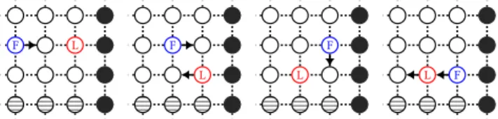
Figure 6: Sequence of configurations during a right turn in an ascending phase.

The last case to study is when the leader reaches a corner after that the group has traversed the line along the top (resp. bottom) wall in an ascending (resp. descending) phase. In this case, the leader detects that the group cannot further move Up (resp. Down). For example, the leader has color 𝐿 but cannot turn Left because the top wall is at its Left. In this case, the leader moves away from the top wall and changes its color in the same step, i.e., it moves Right and takes color 𝑅 if its color was 𝐿, it moves Left and takes color 𝐿 otherwise; see the rules in Fig. 7. Notice also that, after this turn, the leader again changes its color while leaving the wall, using the

previous rules given in Fig. 5. Overall, after turning at such a corner, the leader has changed its color twice, and consequently starts the descending (resp. ascending) phase. An example where the group switches from an ascending to a descending phase (resp. from a descending to an ascending phase) is given in Fig. 8 (resp. Fig. 9).

F L

R

F RL

Figure 7: Moving at a corner.

F L F L

R F

R

L L F

Figure 8: Sequence of configurations during a turn at a cor-ner. F R F R L L F R R F

Figure 9: Sequence of configurations during a turn at an-other corner.

Theorem 4.1. Vone2₃solves the PGFE problem with two robots and three colors.

Proof. By induction on 𝑚 × 𝑛, where 𝑚 is the number of lines and 𝑛 is the number of columns of the grid. We have validated several base cases, including even and odd values for the number of lines, using our simulation tool [6]. Precisely, we have checked that Vone2₃solves the PGFE problem on every grid of size 𝑚 × 𝑛 for 𝑚=2, 3 and 𝑛 = 2. Such a checking is easy since, from a given initial configuration, there is only one possible execution (the algorithm is well-defined and the execution is synchronous). So, we just have to execute the algorithm until reaching an already encountered configuration: at that time all nodes should have been visited.

We assume now that Vone2₃solves the PGFE problem in all grids 𝑥× 𝑦 with 2 ≤ 𝑥 ≤ 𝑚 and 2 ≤ 𝑦 ≤ 𝑛 for some values 𝑚 ≥ 3 and 𝑛≥ 2. We should show that Vone2

3solves the PGFE problem in the grids of size 𝑚 × (𝑛 + 1) and (𝑚 + 1) × 𝑛.

Consider first the grid of size 𝑚 × (𝑛 + 1). Then, it is easy to see that after adding one column, our algorithm still solves the PGFE problem. Indeed, when robots are traveling from the left to the right, they move in a straight line periodically until they reach a wall, so adding one column just increases by one the number of times they perform their periodic movement.

Consider now the grid of size (𝑚 + 1) × 𝑛. Since 𝑚 − 1 ≥ 2, the induction hypothesis applies to the case (𝑚 − 1) × 𝑛, i.e., Vone2₃ solves the PGFE problem in the grid (𝑚 − 1) × 𝑛. Now, we can remark that, after adding two lines, Vone2₃still solves the PGFE. Indeed, every time the robots travel horizontally from one wall to

the other and then come back, they are located exactly two lines above their previous location when they left the wall the first time. For example, assume (0, 0) represents the node at the bottom left corner and consider the grid of size (𝑚 + 1) × 𝑛. If the configuration is 𝐶1= {( (0, 𝑗), 𝐹 ), ((1, 𝑗), 𝐿)} at a given time, with 1 ≤ 𝑗 ≤ 𝑚 − 1, then it is 𝐶2= {( (0, 𝑗 + 2), 𝐹 ), ((1, 𝑗 + 2), 𝐿)} after 2𝑛 rounds. So, the execution is similar from 𝐶1in the grid of size (𝑚 − 1) × 𝑛 and from 𝐶₂in the grid of size (𝑚 + 1) × 𝑛, i.e., adding two lines just implies that they perform this periodic movement one more time. □

5

VISIBILITY RANGE TWO : Vtwo

AND Vtwo

Under visibility range of two, we can reduce the number of colors to two still using two robots; see Subsection 5.1. We can also use only one color, yet with three robots; see Subsection 5.2.

5.1

Algorithm Vtwo

2

The principle of Algorithm Vtwo2₂is similar to that of Algorithm Vone3₂. For example, initially, the leader robot, with color 𝐿, should be adjacent to a follower, with color 𝐹 (n.b., as a consequence, the set of all possible initial configurations is still locally-defined). However, instead of using two colors at the leader to distinguish the right and left wall, we exploit the distance between the leader and the follower. More precisely, when the leader reaches a wall while being adjacent to the follower, the two robots perform a left turn, as illustrated in Fig. 10. Conversely, if the leader is at distance two from the follower when reaching a wall, the two robots perform a right turn, as illustrated in Fig. 11.

L F F

L

F

L F L

Figure 10: Sequence of configurations during a left turn. The same sequence occurs regardless of the presence of a wall at the hatched nodes.

F L F

L

F

L L F

Figure 11: Sequence of configurations during a right turn. The same sequence occurs regardless of the presence of a wall at the hatched nodes.

When traveling from wall to wall, the two robots preserve their distance. The leader moves away from the follower, regardless its distance to the follower, the presence of walls at distance two, or the presence of a wall at distance one on a specific side, as illustrated in Fig. 12. The follower always follows the leader regardless of their distance and the presence of walls, as dictated by rules shown in Fig. 13. The only exception occurs when the follower is adjacent to the leader, and there is a wall adjacent on its right. In that case, the follower stays idle. This is done to separate the leader and the

follower during a left turn. We can see that in the second configu-ration in the sequence shown in Fig. 10, the follower is adjacent to the leader, but stays idle while the leader continues to move. After that, the leader and the follower are at distance two.

L F L F

L F L F

Figure 12: When it sees no walls, the leader moves away from the follower.

L F L F

Figure 13: The follower always follows the leader, except when there is a wall immediately on its right.

The rules executed by the leader when reaching a wall are more specific and depend on its distance to the follower. When the leader reaches a wall and is at distance two (resp. distance one) from the leader, then it turns right (resp. turns left); as shown in Fig. 14.

L F L F

Figure 14: When reaching a wall, the leader either turns right or left depending on its distance with the follower.

If the leader has turned right, the rules shown in Fig. 15 dictate the follower to move towards the wall, while the leader moves away from the wall. Then, the follower moves along the wall towards the leader, and the leader does not move, so that the leader and the follower become adjacent. After that, the leader and the follower are in a configuration from which they move straight towards the opposite wall. The entire sequence is shown in Fig. 11.

L

F L

F

L F

Figure 15: The rules to complete a right turn. After the turn the follower and the leader are adjacent.

If the leader has turned left when it reached the wall, the rules shown in Fig. 16 dictate the leader to move away from the wall while the follower stays idle. Then, the follower moves along the wall towards the leader while the leader moves away from the wall. After that the leader and the follower are at distance two. The entire sequence is shown in Fig. 10.

F

L F

L

F L

Figure 16: The rules to complete a left turn. After the turn the follower and the leader are at distance two.

The remaining rules apply when the robots reach a corner and the phase should change (from ascending to descending, or con-versely). When robots are adjacent and move along a wall on their left side, they move while ignoring the wall until the leader sees a wall in front of it. When this happens, the first rule in Fig. 17 dictates the leader to change its color. After that, both robots have color 𝐹 . Then, they perform a special move to (1) turn around in one round (the second and third rules in Fig. 17) by moving away from the wall, and (2) reverse the leader and follower roles. The complete sequence is illustrated in Fig. 18.

L F

F

F F F LF

Figure 17: The rules to move along a wall when robots are ad-jacent, until reaching a corner and then performing a right turn by switching the leader and follower roles.

L F

F F F

L

F L F L

Figure 18: Sequence of configurations at a corner. The same thing occurs in the opposite direction when robots are not adjacent, using the rules shown in Fig. 19.

F LF LF F F F

Figure 19: The rules to move along a wall when robots are not adjacent, until reaching a corner and then performing a left turn by switching the leader and follower roles.

Finally, there are three rules that are used in specific cases. The first rule in Fig. 20 applies only once in specific initial configurations.

The second rule in Fig. 20 is used when the number of columns or the number of lines is two. When this rule is executed, the robots will move along the wall and the other rules apply as usual. The last rule in Fig. 20 applies only in the grid of size 2 × 2. After this rule is executed, the leader moves to an empty node, while the follower moves to another empty node (by applying an existing rule shown in Fig. 16), hence after one round, the configuration is rotated by 𝜋 /2 so that this occurs infinitely often while each node is visited every two rounds. Those special cases can be visualized in the animation in our complementary material [6].

L F L F

F L

Figure 20: Three rules used in specific cases. Theorem 5.1. Vtwo2₂solves the PGFE problem with two robots, having two colors and visibility range two.

Proof. The induction proof is similar to Theorem 4.1 for Vone3₂. In particular, the base cases have been checked automatically using the same simulation tool [6]. □

5.2

Algorithm Vtwo

Our last algorithm, Algorithm Vtwo1₃, uses three anonymous obliv-ious robots (i.e., three robots with only one color) under visibility range two. The algorithm uses the same principle as the previous ones, but two shapes are used to distinguish what to do when reach-ing a wall. We respectively denote these two shapes by “<” and “L”. We define the set of locally-defined initial configurations as the set of configurations where the robots form an “<” shape. Fig. 21 (resp. Fig. 22) shows the rules executed by the robots to move straight when in the “<” shape (resp. when in the “L” shape). With those rules, robots are able to move straight, regardless of the presence of wall “behind” them, or on their “side”.

R R R R R R R R R

Figure 21: Rules to move straight for an “<” shape.

R

R R

R

R R R

R R

Figure 22: Rules to move straight for a “L” shape. When a robot reaches a wall, the robots “turn around”. When two robots become adjacent to a wall while robots are in an “<” shape,

two robots move down (if the wall is on the right in the global view), so that the robots now form an “L” shape; as illustrated in the sequence of configurations in Fig. 23. The rules executed by the robots during this turn are shown in Fig. 24.

R R R R R R R R R R R R

Figure 23: Sequence of configurations when robots in an “<” shape reach a wall.

R R R R R R

Figure 24: Rules to turn when robots are in an “<” shape. When a robot becomes adjacent to a wall while robots are in an “L” shape, it moves down (if the wall is left in the global view) while another robot remains idle and the last one continues to move towards the wall (because it does not see the wall as it is obstructed). After that, the bottommost robot moves away from the wall so that the robots form an “<” shape; as illustrated in the sequence of configurations in Fig. 25. The rules executed by the robots during this turn are shown in Fig. 26.

R R R R R R R R R R R R

Figure 25: Sequence of configurations when robots in a “L” shape reach a wall.

R

R R

R R

Figure 26: Rules to turn when robots are in a “L” shape. When the robots cannot perform a turn at a corner, they perform a turn around without changing their shape. This always occurs when they are in an “<” shape. The robot at the corner moves away towards the position from it came from, the robot in the middle moves up (instead of down during a standard turn), and the topmost robot, which does not see the corner, moves down as usual; as illustrated in the sequence of configurations in Fig. 27. The rules executed by the robots during this turn are shown in Fig. 28.

R R R R R R R R R R R R

Figure 27: Sequence of configurations when robots in an “<” shape reach a corner.

R R R R R R

Figure 28: Rules to turn at a corner.

Theorem 5.2. Vtwo1₃solves the PGFE problem with three robots, having only one color and visibility range two.

Proof. The induction proof is similar to Theorem 4.1 for Vone3₂. In particular, the base cases have been checked automatically using the same simulation tool [6]. □

6

CONCLUSION

We have proposed optimal synchronous solutions to the exclusive PFGE problem for swarms of luminous myopic opaque robots. The optimal algorithm Vone3₂for visibility range one requires only two robots and three colors. Yet, if we increase the visibility range to two, we can either decrease the number of colors to two (Algorithm Vtwo2₂), or decrease the number of colors to one (Algorithm Vtwo1₃) but at the price of using one additional robot. We now present some extensions and perspectives.

Asynchronous version of Algorithm Vone3₂. In the asynchronous model, a Look-Compute-Move cycle is not atomic, yet each of the three phases of a cycle is. At each round, a robot executes at most one of the phases. The time between Look, Compute, and Move phases at a given robot is finite yet unbounded.

Algorithm Vone3₂can be modified to work in the asynchronous model, yet using visibility range two. For this, the rules of the leader remain the same: the leader moves if and only if it sees that the follower was its neighbor in its previous Look phase. In contrast, the follower now moves if and only if it sees the leader at distance two in its previous look phase. In this case, it moves toward the leader, as in the synchronous algorithm. It is easy to see that this version works in the asynchronous model since all the robot movements are sequential: each move of the synchronous algorithm is emulated with exactly two moves in the asynchronous one.

From perpetual to terminating exploration. We can simply modify our non-oblivious algorithms so that they terminate once all nodes have been visited. We just have to duplicate states of the follower (four times) to encode in them the number of corners it has already visited and modify the rules accordingly. Using this encoding, when the follower detects that it has reached a corner for the fourth time, it definitely stops. Seeing the follower in a terminating state, the leader also stops. Since the follower has visited the four corners, we have the guarantee that all nodes have been visited meanwhile.

Perspectives. First, one can study the impact of removing the common chirality on the lower bounds. Then, optimality for the terminating variants needs to be investigated. In particular, find-ing an optimal (w.r.t. the number of robots) anonymous oblivious terminating solution under the small visibility range two seems to be quite challenging. Finally, even if we have already given some hints, the designing of asynchronous efficient solutions, still in the myopic context, is definitely the most exciting perspective.

REFERENCES

[1] Roberto Baldoni, François Bonnet, Alessia Milani, and Michel Raynal. 2008. Anonymous graph exploration without collision by mobile robots. Inf. Process. Letters 109, 2 (2008), 98–103.

[2] Lélia Blin, Alessia Milani, Maria Potop-Butucaru, and Sébastien Tixeuil. 2010. Exclusive Perpetual Ring Exploration without Chirality. In Distributed Computing, 24th International Symposium, DISC 2010, Cambridge, MA, USA, September 13-15, 2010. Proceedings, Nancy A. Lynch and Alexander A. Shvartsman (Eds.), Vol. 6343. Springer, Boston, Massachusetts, USA, 312–327.

[3] François Bonnet, Alessia Milani, Maria Potop-Butucaru, and Sébastien Tixeuil. 2011. Asynchronous exclusive perpetual grid exploration without sense of di-rection. In Proceedings of International Conference on Principles of Distributed Systems (OPODIS 2011), Antonio Fernández Anta (Ed.). Springer Berlin / Hei-delberg, Toulouse, France, 251–265. http://www.springerlink.com/content/ 9l3v424157681707/

[4] Quentin Bramas, Stéphane Devismes, and Pascal Lafourcade. 2020. Finding Water on Poleless using Melomaniac Myopic Chameleon Robots. In FUN 2020, 10th International Conference on Fun with Algorithms. LiPICs, Favignana, Sicily, Italy. to appear.

[5] Quentin Bramas, Stéphane Devismes, and Pascal Lafourcade. 2020. Infinite Grid Exploration by Disoriented Robot. In NETYS’2020, the 8th International Conference on NETworked sYStems. Springer, Marrakech, Morocco. to appear.

[6] Quentin Bramas, Stéphane Devismes, and Pascal Lafourcade. 2020. Optimal Exclusive Perpetual Grid Exploration by Luminous Myopic Opaque Robots: The Animations. https://doi.org/10.5281/zenodo.3947756.

[7] Ajoy Kumar Datta, Anissa Lamani, Lawrence L. Larmore, and Franck Petit. 2015. Enabling Ring Exploration with Myopic Oblivious Robots. In 2015 IEEE Interna-tional Parallel and Distributed Processing Symposium Workshop, IPDPS 2015. IEEE Computer Society, Hyderabad, India, 490–499.

[8] Stéphane Devismes, Anissa Lamani, Franck Petit, Pascal Raymond, and Sébastien Tixeuil. 2020. Terminating Exploration of a Grid by an Optimal Number of Asynchronous Oblivious Robots. Comput. J. 1 (03 2020). to appear.

[9] Stéphane Devismes, Anissa Lamani, Franck Petit, and Sébastien Tixeuil. 2019. Optimal torus exploration by oblivious robots. Computing 101, 9 (2019), 1241– 1264.

[10] Stéphane Devismes, Franck Petit, and Sébastien Tixeuil. 2013. Optimal Proba-bilistic Ring Exploration by Semi-synchronous Oblivious Robots. Theoretical Computer Science (TCS) 498 (2013), 10–27.

[11] Yoann Dieudonné, Franck Petit, and Vincent Villain. 2010. Leader Election Problem versus Pattern Formation Problem. In Distributed Computing, 24th Inter-national Symposium, DISC 2010, Nancy A. Lynch and Alexander A. Shvartsman (Eds.), Vol. 6343. Springer, Cambridge, MA, USA, 267–281.

[12] Paola Flocchini, David Ilcinkas, Andrzej Pelc, and Nicola Santoro. 2010. Remem-bering without memory: Tree exploration by asynchronous oblivious robots. Theor. Comput. Sci. 411, 14-15 (2010), 1583–1598.

[13] Paola Flocchini, David Ilcinkas, Andrzej Pelc, and Nicola Santoro. 2011. How many oblivious robots can explore a line. Inf. Process. Lett. 111, 20 (2011), 1027– 1031.

[14] Paola Flocchini, David Ilcinkas, Andrzej Pelc, and Nicola Santoro. 2013. Com-puting Without Communicating: Ring Exploration by Asynchronous Oblivious Robots. Algorithmica 65, 3 (2013), 562–583.

[15] Fukuhito Ooshita and Sébastien Tixeuil. 2018. Ring Exploration with Myopic Luminous Robots. In Stabilization, Safety, and Security of Distributed Systems -20th International Symposium, SSS 2018, Taisuke Izumi and Petr Kuznetsov (Eds.), Vol. 11201. Springer, Tokyo, Japan, 301–316.

[16] David Peleg. 2005. Distributed Coordination Algorithms for Mobile Robot Swarms: New Directions and Challenges. In Distributed Computing – IWDC 2005, Ajit Pal, Ajay D. Kshemkalyani, Rajeev Kumar, and Arobinda Gupta (Eds.). Springer Berlin Heidelberg, Berlin, Heidelberg, 1–12.

A

OMITTED PROOFS

We first give a simple technical lemma that makes easier our im-possibility proofs.

Lemma 3.1. Let A = (Cl, Init, 𝑇 ) be an algorithm that solves the PFGE problem using 𝑛 robots. For every grid 𝐺 with at least 𝑛 lines and 𝑛 columns, for every node 𝑢 in 𝐺, there exist a configuration 𝐶 where a robot is located at 𝑢 and an algorithm A′ = (Cl, Init′, 𝑇) where Init′is identical to Init unless 𝐶 ∈ Init′(𝐺) such that A′solves the PFGE problem using 𝑛 robots.

Proof. Let 𝑢 be a node of 𝐺. If A solves the PFGE problem in 𝐺, then there is an execution 𝐶1, 𝐶₂, . . . , 𝐶_𝑘, . . .starting from 𝐶₁∈ Init (𝐺) such that 𝑢 is occupied in 𝐶𝑘.

Let 𝜀′= 𝐶₁′(= 𝐶𝑘), 𝐶₂′, . . .an arbitrary execution suffix starting from 𝐶𝑘. Then, 𝐶1, . . . , 𝐶_𝑘, 𝐶′

2, 𝐶 ′

3, . . .is a possible execution of A starting from 𝐶1. By hypothesis, each node is visited infinitely often in this execution, and so is in 𝜀′. Hence, if we add 𝐶𝑘as a possible initial configuration, we still have an algorithm that solves the PFGE

problem in 𝐺. □

Lemma A.1. Consider any algorithm A that solves the PFGE prob-lem with three robots, one color, and visibility range one.

No execution of A contains a configuration where the three robots are isolated and do not see any wall.

Proof. Assume, by the contradiction, that an execution of A reaches a configuration 𝐶 where the three robots are isolated and do not see any wall. By Lemma 3.1, we can assume, without the loss of generality, that 𝐶 is this initial configuration.

Assume first that a robot remains idle in 𝐶. Now, since each robot has the same color and the same local view. All robots are idle forever, a contradiction.

Assume now that a robot is enabled to move in 𝐶. Again, each robot has the same color and the same local view, so all robots are enabled to move. Moreover, for each robot, each possible destina-tion looks identical. Consider then the smallest rectangle 𝑅 that encloses the three robots. There exist three transformations such that applying each one to a robot make them move in such a way that they are still isolated and inside 𝑅 in the reached configuration 𝐶′. In particular, they still do not see any wall in 𝐶′. So, by repeating the same mechanism, we construct a possible execution starting from 𝐶 where several nodes are never visited (precisely, all nodes outside 𝑅), a contradiction. □ Theorem 3.6. The PFGE problem is not solvable with three robots, one color, and visibility range one.

Proof. Assume, by the contradiction, that an algorithm A solves the PFGE problem with three robots, one color, and visibility range one. Let 𝑟1, 𝑟2, and 𝑟3be the three robots. Consider a grid 𝐺 of size at least 22 × 22 whose number of lines or columns is even. By Lemma 3.1 (recall thatΦ = 1), we can assume, without the loss of generality, that A solves the PFGE problem starting from an initial configuration 𝐶 where a robot is located at a center of 𝐺.

Claim 1: There is an execution starting from 𝐶 containing a configuration where the robots are all at distance at least 6 from any wall.

Proof of the claim: Let 𝑟1be the robot located at a center of 𝐺in 𝐶, hence at distance at least 11 from any wall. We have two possibles cases in 𝐶:

• In 𝐶, 𝑟1sees a robot, say 𝑟2. So, 𝑟2is at distance at least 10 from any wall. So, if 𝑟3is at distance at most 4 from 𝑟2, we are done. Assume now that 𝑟3 is at distance at least 5 from 𝑟2. Then, in the next step, 𝑟1and 𝑟2either stay idle, swap their positions, or become isolated, yet still at distance at least 10 and 9 respectively from any wall. After this step, if 𝑟3is at distance at least 6 from a wall, we are done. Otherwise, 𝑟3is at least at distance 5 and 4 from 𝑟1and 𝑟2respectively. If 𝑟1and 𝑟2are isolated, either they remain idle, or they move but all positions look identical in their respective snapshot. For each of them, there is a transformation that makes them retrieves their initial position. If they are adjacent (they were idle or swapped their position), then they remains adjacent by performing again the same move. Hence, there exists a possible execution where while 𝑟3is not at distance at least 6 from a wall, 𝑟1(resp. 𝑟2) can at most alternate between two neighboring positions. In this execution, a node at distance 6 from a wall is visited first by 𝑟3, and when it happens, all robots are at distance at least 6 from any wall. • 𝑟1is isolated in 𝐶. While isolated, 𝑟1is either idle, or there is a possible step where it moves to a neighboring center, thus remaining at distance 11 from any wall. Hence, in such an execution, there is a node at distance 9 from any wall that is visited first by another robot, say 𝑟2. When it happens, either all robots are at distance 6 from a wall and we are done, or 𝑟1and 𝑟2are both isolated and there exists a possible execution suffix where they both alternates between two positions without seeing a wall while they are isolated: the two centers at distance 11 from any wall for 𝑟1and nodes at distance 9 and 8 from any wall for 𝑟2. In such an execution, a node at distance 7 from a wall is then eventually visited by 𝑟3and when it happens, we are done.

Claim 2: If initially no robot is isolated and all robots are at distance at least 6 from any wall, then there is a reachable configuration where all robots are at distance at least 4 from any wall and at least one of them is isolated.

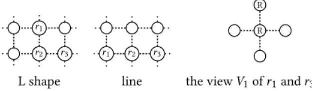
Proof of the claim: Since initially no robot is isolated, there are only two kinds of possible initial configurations for the three robots: either they form a line, or an L shape, as illustrated in Fig. 29.

We now consider an execution with well-chosen transfor-mations such that every time a robot sees only one another robot, its local view is exactly 𝑉1in Fig. 29. In the two kinds of possible initial configurations, there are two robots, say 𝑟₁and 𝑟3, with the same view 𝑉1, so their destinations are opposite in a line configuration, and rotated by 𝜋 /2 in the L configuration. Hence, they cannot move Up in 𝑉1, i.e., to-wards 𝑟2, otherwise they create a collision. If they move Down in 𝑉1, i.e., away from 𝑟2, then at least one of them be-comes isolated, and we are done. We now show that moving Left or Right in 𝑉1also leads to at least one robot becoming isolated. If the three robots initially form a line and if 𝑟1and

𝑟₁

𝑟₂ 𝑟₃ 𝑟₁ 𝑟₂ 𝑟₃

R

R

L shape line the view 𝑉1of 𝑟1and 𝑟3 Figure 29: The two possible configurations where three robots are connected, and the view of the robots 𝑟1 and 𝑟3 in both cases. 𝑟₁ 𝑟₂ 𝑟₃ 𝑟₁ 𝑟₃ 𝑟₂

Figure 30: In an L shape, if robots 𝑟1and 𝑟3with view 𝑉1move left, then, 𝑟2has to move right not to isolate 𝑟1.

𝑟₃move on the Right or the Left in 𝑉1, then at least one of them becomes isolated. If they do not move and 𝑟2moves without colliding, 𝑟2becomes isolated. If no robots move, we have a deadlock and so the exploration fails, a contradiction. If the three robots initially form an L shape and if 𝑟1and 𝑟3 move Left on 𝑉1, then in the global view illustrated in Fig. 30, 𝑟₃moves down and 𝑟₁moves right. In this case, if 𝑟2moves towards 𝑟3, the robots form a line and we retrieve a previous case. Otherwise, 𝑟1or 𝑟3becomes isolated; see Fig. 30. The same thing happens if 𝑟1and 𝑟3move Right in 𝑉1. Overall, since the robots were initially all at distance at least 6 from any wall, after one or two rounds they are at distance at least 4 from any wall and at least one of them is isolated. Claim 3: In all reachable configurations where all robots are at

distance at least 4 from any wall, no robot is isolated. Proof of the claim: Assume by the contradiction that there is an execution where the configuration at time 𝑡 satisfies the following two conditions: (1) all robots are at distance at least 4 from any wall and (2) one robot, say 𝑟3, is isolated. Then, the two other robots 𝑟1and 𝑟2are adjacent, otherwise we obtain a contradiction Lemma A.1. Thus, in the next step, 𝑟1 and 𝑟2are either idle, swap their positions, or move to be at distance 3 from one another. In the first two cases, 𝑟3either stays idle or can alternate between two nodes (using the appropriate transformations) without seeing the two other robots, so there is an execution suffix where at most 4 nodes are visited, a contradiction. In the third case, while 𝑟1and 𝑟2 are moving away from each other, 𝑟3either moves or is idle. We assume that, if 𝑟3moves between 𝑡 and 𝑡 + 1, then we apply a transformation that makes it move away from 𝑟1and 𝑟₂so that, in this case, it remains isolated at time 𝑡 + 1. So, at time 𝑡 + 1, either each robot becomes isolated, or a robot, say 𝑟2, becomes adjacent to 𝑟3at time 𝑡 + 1, but in this case 𝑟3 was necessarily idle in the step from 𝑡 to 𝑡 + 1. In the former case, we obtain a contradiction by Lemma A.1 again since no robot see a wall. In the latter case, 𝑟2and 𝑟3are adjacent at time 𝑡 + 1 and are necessarily both at distance at least 3 from 𝑟1(n.b., as 𝑟3has stand idle, it was at distance 2 from

𝑟₂and so at distance at least 3 from 𝑟1and by moving in this opposite direction from 𝑟2, 𝑟1has necessarily increased its distance to 𝑟3by one). So, 𝑟2and 𝑟3at time 𝑡 + 1 have exactly the same view as 𝑟1and 𝑟2at time 𝑡 hence execute the same rules and move at distance 3 from each other. Moreover, 𝑟1is necessarily idle at time 𝑡 + 1 since it is in the same situation as 𝑟3at time 𝑡 . So all the robots become isolated at time 𝑡 + 2 (recall that 𝑟1and 𝑟2are at distance 3 at time 𝑡 + 1). Overall, it is possible to make all robots isolated within at most two steps from time 𝑡 . Now, all robots were at distance at least 4 from any wall at time 𝑡 . So, in such a case, they still not see any wall after the two steps and we obtain a contradiction by Lemma A.1.

By Lemma 3.1 and Claim 1, we can assume, without loss of generality, robots are initially in a configuration 𝐶0where they are all at distance at least 6 from any wall. By Lemma A.1, not all robots are isolated in 𝐶0. Moreover, by Claim 2, there is a configuration 𝐶𝑖 reachable from 𝐶0where (1) all robots are at distance at least 4 from any wall and (2) at least one of them is isolated, contradicting then Claim 3.