BRIDGE: Matching Model Based Diagnosis from FDI and DX perspectives

(1)

HAL Id: hal-03089393

https://hal.laas.fr/hal-03089393

Submitted on 13 Jan 2021

HAL is a multi-disciplinary open access

archive for the deposit and dissemination of

sci-entific research documents, whether they are

pub-lished or not. The documents may come from

teaching and research institutions in France or

abroad, or from public or private research centers.

L’archive ouverte pluridisciplinaire HAL, est

destinée au dépôt et à la diffusion de documents

scientifiques de niveau recherche, publiés ou non,

émanant des établissements d’enseignement et de

recherche français ou étrangers, des laboratoires

publics ou privés.

and DX perspectives

Louise Travé-Massuyès, Teresa Escobet

To cite this version:

Louise Travé-Massuyès, Teresa Escobet. BRIDGE: Matching Model Based Diagnosis from FDI and

DX perspectives. Teresa Escobet; Anibal Bregon; Belarmino Pulido; Vicenç Puig. Fault Diagnosis

of Dynamic Systems. Quantitative and Qualitative Approaches, Springer International Publishing,

pp.153-175, 2019, 978-3-030-17727-0. �10.1007/978-3-030-17728-7_7�. �hal-03089393�

(2)

Fault Diagnosis

of Dynamic Systems

Teresa Escobet

Anibal Bregon

Belarmino Pulido

Vicenç Puig

January 16, 2019

(3)

BRIDGE: Matching Model Based Diagnosis

from FDI and DX perspectives

Louise Travé-Massuyès and Teresa Escobet

7.1 Introduction

As introduced in Chapter 1, the goal of diagnosis is to identify the possible causes explaining a set of observed symptoms. The following three tasks are commonly identified:

• fault detection discriminates normal system states from faulty states, • fault isolation, also called fault localization, points at the faulty components, • fault identification, identifies the type of fault.

Several scientific communities have addressed these tasks and contributed with a large spectrum of methods, in particular the Signal Processing, Control, and Arti-ficial Intelligence (AI) communities. Diagnosis spreads from the signal acquisition level up to levels in which relevant abstractions are used to interpret the available signals qualitatively.

Qualitative interpretations of the signals exist in terms of symbols or events. To do that, discrete formalisms borrowed from AI find a natural link with continuous models from the Control community. Different facets of diagnosis investigated in the Control or the AI fields have been discussed in the literature. [24–26] provide three interesting surveys of the different approaches that exist in these fields. These two communities have their own model-based diagnosis track:

• the FDI (Fault Detection and Isolation) track, whose foundations are based on engineering disciplines, such as control theory and statistical decision making,

Louise Travé-Massuyès

LAAS-CNRS, Université de Toulouse, CNRS, Toulouse, France, e-mail:[email protected]

Teresa Escobet

Department of Mining, Industrial and ICT Engineering; Research Center for Supervision, Safety and Automatic Control, Universitat Politècnica de Catalunya, e-mail:teresa.escobet@upc. edu

(6)

• the DX (Diagnosis) track, whose foundations are derived from the fields of logic, combinatorial optimization, search and complexity analysis.

There has been a growing number of researchers in both communities who have tried to understand and bridge FDI and DX approaches to build better, more robust and effective diagnostic systems. In particular, the concepts and results of the FDI and DX tracks have been put in correspondence and the lessons learned from this comparative analysis pointed out.

The FDI and DX streams both consider the diagnosis problem from a system point of view, which results in significant overlaps. Even the name of the two tracks are the same : Model-Based Diagnosis (MBD). This chapter presents and examines this "bridge".

The diagnosis principles are the same, although each community has devel-oped its own concepts and methods, guided by different modeling paradigms and solvers. FDI relies on analytical models, linear algebra, and non-linear system the-ory whereas DX takes its foundations in logic.

In the 2000s, although the common goals were quite clear, the underlying con-cepts and the procedures of the two fields would remain mutually obscure. There were more and more researchers who tried to understand and synergistically inte-grate methods from the two tracks to propose more efficient diagnostic solutions.

The chapter is organized as follows. After the introduction section, section7.2

first presents a brief overview of the approaches proposed by the FDI and DX model-based diagnosis communities. Although quite commonplace, this overview is neces-sary because it provides the basic concepts and principles that form the foundations of our comparative analysis. It is followed by the comparison of the mathematical objects used as input of the diagnosis procedures. Section7.3then establishes the correspondances of concepts on both sides and compares the techniques used by the two communities. Interestingly, the results obtained by the two approaches are shown to be the same under some assumptions that are exhibited. Finally, Section

7.4illustrates the DX-FDI MBD bridge with the classical example of the polybox.

7.2 DX and FDI MBD approaches

Both the FDI and DX communities have a Model-Based Diagnosis (MBD) track which can be put in correspondence. After a brief reminder of the concepts of the two tracks, this section compares the models used on each side and the sets the assumptions that are adopted to favor the comparative analysis.

7.2.1 Brief overview of the FDI approach

This section briefly summarizes the concepts presented in Chapter 3.6. The FDI community generally deals with dynamic systems represented by behavioral models

(7)

that relate system inputs u 2 U and outputs y 2 Y, gathered in the set of measurable variables Z, and system internal states defining the set of unknown variables X . The variables z 2 Z and x 2 X are functions of time. The typical model can be formulated in the temporal domain, then known as a state-space model :

BM : dx/dt = f (x(t),u(t),✓)

OM :y(t) = g(x(t),u(t),✓). (7.1) wherex(t) 2 <nx _{is the state vector,}u(t) 2 <nu _{is the input vector and}y(t) 2 <ny _is

the output vector. Thenz(t) = (u(t),y(t))T_{. ✓ 2 <}n✓ is a constant parameter vector.

The components of f and g are real functions over <. BM is the behavioral model and OM is the observation model. The whole system model is noted SM(z,x), like in [13], and assumed noise-free. The equations of SM(z,x) may be associated to components but this information is not represented explicitly. The models can also be formulated in the frequency domain, for instance in the form of transfer functions in the linear case.

Model (7.1) can be illustrated by the example of two coupled water tanks Ttand Tb. Ttis the top tank and its output fills the bottom tank Tb:

BM :⇢x1(t) = a1˙ u(t)- a2px1(t), ˙ x2(t) = a3px1(t)- a4px2(t), (7.2) OM : ⇢ y1(t) = px1(t), y2(t) = px2(t). (7.3) where ai,i = 1,...,4, ai6= 0, are model parameters. x(t) = (x1(t),x2(t))T _represents the state vector and corresponds to the level in each tank, u(t) 6⌘ 0 is the input vector, andy(t) = (y1(t),y2(t))T _{is the output vector. Measurable variables are given by the} vectorz(t) = (u(t),y1(t),y2(t))T_.

The books [10], [4], [8], [16] provide excellent surveys, which cite the origi-nal papers that the reader is encouraged to consult. The paper [26] also provides a quite comprehensive survey. The equivalence between observers, parity space and paramater estimation has been proved in the linear case [15].

The concept central to FDI methods is the concept of residual and one of the main problems is to generate residuals. Residual generators are defined in Definition3.15

of Chapter2.6and this definition is recalled below.

Definition 7.1 (Residual generator for SM(z,x)). A system that takes as input a sub-set of measured variables ˜_{Z ✓ z and generates as output a scalar r, is a residual} generator for the model SM(z,x) if for all z consistent with SM(z,x), limt!+1r(t) =

0.

Let’s consider the model SM(z,x) given by (7.1), then SM(z,x) is said to be con-sistent with an observed trajectoryz, or simply consistent with measurements z, if there exists a trajectory ofx such that the equations of SM(z,x) are satisfied. The residuals tend to zero as t tends to infinity when the system model is consistent with measurements, otherwise some residuals may be different from zero. In practice, noises may affect the residuals that are never exactly zero. Indeed, the noise-free

(8)

assumption adopted for (7.1) is never met. Statistical tests that account for the sta-tistical characteristics of noise [3,8] are used to evaluate the residuals as a Boolean value 0 or 1. The residuals are often optimized to be robust to disturbances [18] and to take into account uncertainties [1]. The reader can refer to Chapter3.6and9.6for more details about how to deal with uncertainty, using decoupling methods or with interval methods respectively.

Among the three standard FDI approches, the Bridge comparison is carried out based on the so-called parity space approach [5]. In this approach, residuals are generated from relations that are inferred from the system model by eliminating un-known variables, i.e. state variables. These relations, called Analytical Redundancy Relations (ARR), are determined off-line. ARRs are constraints that only involve measured input and output variables and their derivatives. For linear systems, ARRs are obtained eliminating unknown state variables by linear projection on a particular space, called the parity pace [5]. An extension to non-linear systems is proposed in [21]. On the other hand, structural analysis [2,22] is an interesting approach because it allows one to obtain, for linear or non-linear systems, the just overdeterminated sets of equations from which ARRs can be derived (see2.6).

Every ARR can be put in the form r(t) = 0, where r(t) is the residual.

For the two tanks system (7.2)-(7.3), the two following residuals can be obtained from the Rosenfeld-Groebner algorithm as explained in [7]:

r1(t) =-a1u+ a2y1+ 2y1y1,˙

r2(t) = a4y2- a3y1+ 2y2y2˙ . (7.4) If the behavior of the system satisfies the model constraints, then the residuals are zero because the ARRs are satisfied. Otherwise, some of them may be different from zero when the corresponding ARRs are violated. Given a set of n residuals, a theoretical fault signature FSj= [s1 j,s2 j, . . . ,sn j] given by the Boolean evaluation of each residual is associated to each fault Fj. Note that Fjmay be a simple or multiple fault. The signature matrix is then defined as follows.

Definition 7.2 (Signature Matrix). Given a set of n ARRs, the signature matrix FS associated to a set of nf faults F = [F1,F2, . . . ,Fnf] is the matrix that crosses

corresponding residuals as rows and faults as columns, and whose columns are given by the theoretical signatures of the faults, i.e. FS = [FS1,FS2, . . . ,FSn_f].

In the two tanks example system (7.2)-(7.3), let us consider a fault fT_bon the bot-tom tank, i.e. a leak lb, and a fault fTt on the top tank, i.e. a leak lt. The leak lbof the

bottom tank impacts residual r1(t) whereas the leak lt of the top tank impacts both residuals r1(t) and r2(t). The multiple fault composed of the two leaks obviously affects the two residuals as well. The signature matrix is hence given in Table7.1.

Diagnosis is achieved by matching the observed signature, i.e. the Boolean resid-ual values obtained from the actresid-ual measurements, to one of the theoretical signa-tures of the nf faults.

(9)

Table 7.1 Fault signature of the two tanks system. fTb fTt fTbTt

r1(t) 1 1 1

r2(t) 0 1 1

7.2.2 Brief overview of the DX logical diagnosis theory

In the model-based logical diagnosis theory of DX as proposed by [12,19] and presented in depth in Chapter4.5.2, the description of the system is driven by com-ponents and relies, in its original version, on first order logic. A system is given by a tuple (SD,COMPS,OBS) where:

• SD is the system description in the form of a set of first order logic formulas with equality,

• COMPS represents the set of components of the system given by a finite set of constants,

• OBS is a set of first order formulas, which represent the observations.

SD uses the specific predicate AB, meaning abnormal. Applied to a component c of COMPS, ¬AB(c) means that c is normal and AB(c) that c is faulty. For instance, the model of a two inputs adder would be given by:

¬AB(x) ^ ADD(x) ) out(x) := in1(x)+ in2(x) (7.5)

Definition 7.3 (Diagnosis). A diagnosis for the system (SD,COMPS,OBS) is a set ✓ COMPS such that SD [ OBS [ {AB(c) | c 2 } [ {¬AB(c) | c 2 OBS - } is satisfiable.

The above definition means that the assumption stating that the components of are faulty and all the others are normal is consistent with the observations OBS and the system description SD. A diagnosis hence consists in the assignment of a mode, normal or faulty1_{, to each component of the system, which is consistent with the}

model and the observations.

Definition 7.4 (Minimal diagnosis). A minimal diagnosis is a diagnosis such that 8 0_{⇢ ,} 0_{is not a diagnosis.}

To obtain the set of diagnoses, it is usual to proceed in two steps, basing the first step on the concept of introduced in [19] and later extended in [12]. The original definition, that we call R-conflict, i.e. conflict in the sense of Reiter, is the following : Definition 7.5 (R-conflict and minimal R-conflict). An R-conflict is a set C ✓ COMPS such that the assumption that all the components of C are normal is not consistent with SD and OBS. A minimal R-conflict is an R-conflict that does not contain any other conflict.

(10)

The set of diagnoses can be generated from the set of conflicts. [19] proved that minimal diagnoses are given by the hitting sets2_{of the set of minimal R-conflicts.}

An algorithm based on the construction of a tree, known as the HS-tree, was origi-nally proposed in [19].

The parsimony principle indicates that preference should be given to minimal diagnoses. Another reason why minimal diagnoses are important is because in many cases, they characterize the whole set of diagnoses. In other words, all the supersets of minimal diagnoses are diagnoses. The conditions for this to be true were provided in [12] by extending the definition of an R-conflict to a disjunction of AB-literals, AB(c) or ¬AB(c), containing no complementary pair, entailed by SD [ OBS. Then, a positive conflict is a conflict for which all of its literals are positive and one can identify a with an R-conflict [19] as defined above.

Diagnoses are characterized by minimal diagnoses if and only if all minimal con-flicts are positive [12]. Unfortunately, only sufficient conditions exist on the syntac-tic form of SD and OBS. One of those is that the clause form of SD [ OBS only contains positive AB-literals. This is verified, for instance, if all sentences of SD are of the same form as (7.5), which means that only necessary conditions of correct behavior are expressed.

7.2.3 Modeling comparison

Given the frameworks defined in Sections7.2.1and7.2.2, it is important to com-pare the models that are used on both sides to represent the knowledge useful to diagnosis. Three dimensions can be analyzed:

• the system representation, • observations,

• and, faults.

7.2.3.1 System reperesentation

The modeling paradigm of FDI does not make explicit use of the concept of com-ponent, the system model SM is composed of the behavior model BM and the ob-servation model OM of the non faulty system. The behavioral model (7.1) describes the system as a whole. On the contrary, the DX approach models every compo-nent independently, and specifies the structure of the system, i.e. how the different components are connected. Another important difference is that the assumption of correct behavior is represented explicitly in SD thanks to the predicate AB. If F is a formula describing the normal behavior of a component, SM only contains F whereas SD contains the formula ¬AB(c) ) F.

(11)

The comparison of the two approaches is only possible if the models on both sides represent the same system and the observations/measurements capture the same reality. This is formalized by the System Representation Equivalence (SRE) property introduced in [6], which requires that SM is obtained from SD by setting to false all the occurrences of the predicate AB. It is also assumed that the same observation language is used, i.e. OBS is a conjunction of equality relations, which assign a value to every measured variable.

7.2.3.2 Observations

In DX, the set of observations expresses as a set of first-order formulas. It is hence possible to express disjunctions of observations, which provides a powerful lan-guage. However, very often, only conjunctions of atomic formulas are used. In FDI, the observations are always conjunctions of equalities assigning a real value and/or possibly an interval value to an observed variable. In the following, to favor the comparative analysis, we do assume that we have the same observation language. In both FDI and DX approaches, OBS is identical and made up of relations OBS =z.

7.2.3.3 Faults

DX adopts a component-centered modeling approach and defines a diagnosis as a set of (faulty) components. In FDI the concept of component is not central. FDI represents faults as variables that are explicitly involved in the equations of BM and/or OM [9]. For deterministic models, fault variables can be associated: • to parameters, indicating that the parameter changes value when the fault is

present, in which case they are referred as multiplicative faults,

• to input and/or output variables, indicating actuators and sensors faults, in which case they are referred as additive faults.

FDI faults rather correspond to the DX concept of fault mode. In general, several parameters can be associated with a given component, giving rise to different fault modes. FDI faults are viewed as deviations with respect to the models of normal behavior whereas in the DX’s logical view the faulty behavior cannot be predicted from the normal model.

The parameters of FDI models may not have straightforward physical semantics. The model developer must be able to link model parameters to physical parameters to perform fault isolation.

Note that the DX approach can account for parametric faults by expressing the model at a finer level. For instance, considering a single-input single-output (static) component c whose behavior depends on two parameters ✓1 and ✓2, the standard DX model given by:

(12)

could be replaced by:

COMPS(x) ^ PARM1(y) ^ PARM2(z) ^ ¬AB(x) ^ ¬AB(y) ^ ¬AB(z) ) out(x) = f (in(x),y,z) PARM1(✓1),PARM2(✓2),COMPS(c)

(7.7)

The component-based DX approach can hence be generalized by allowing the set COMPS to include not only components (including sensors and actuators), but also parameters.

7.3 DX and FDI model-based diagnosis Bridge

This section provides the theoretical links and an analysis of the diagnosis results of the DX approach and the parity space FDI approach as presented in [6,23]. Practical comparison and potential synergies are also discussed.

7.3.1 ARR vs. R-conflict

In the two approaches, diagnosis is triggered when discrepancies occur between the modeled (correct) behavior and the observations (OBS). As seen in Section7.2, the detection of discrepancies corresponds to:

• R-conflicts in DX,

• ARRs that are not satisfied by OBS in FDI.

The fault signature matrix FS, as defined in Definition7.2, can be used to explain the relation between R-conflicts and ARRs. FS crosses ARRs in rows and faults/-components in columns (here faults are univocally associated to faults/-components). The concept of ARR Support is also necessary.

Definition 7.6 (ARR Support). Consider ARRito be an ARR for SM(z,x), then the support of ARRi, noted supp(ARRi), is the set of components {cj} (columns of the signature matrix FS) whose corresponding matrix cells FSi j are non zero on the ARRiline.

The support of an ARR of the form r(z,˙z,¨z,...) = 0 indicates the set of com-ponents whose models, or submodels, are involved in the obtention of the relation r(z,˙z,¨z,...) = 0. The equations of the model SM(z,x) can indeed be partitioned in component models and every equation of SM(z,x) can be labelled as being part of the model of some component. Let SM(C) denote the subset of equations defin-ing the model of a component c 2 COMPS and SM(C) =Sc2CSM(c) the subset of equations corresponding to C ✓ COMPS.

(13)

A2 A1 M a e b d f g c

Fig. 7.1 Small polybox example.

Let us now introduce two completeness properties, which refer to detectability indicated by a d, and to isolability indicated by an i.

Property 7.1 (ARR–d–completeness). A set E of ARRs is said to be d-complete if: • E is finite;

• 8OBS, if SM [ OBS |=?, then 9ARRi2 E such that {ARRi} [ OBS |=?.

Property 7.2 (ARR–i–completeness). A set E of ARRs is said to be i-complete if: • E is finite;

• 8C, set of components such that C ✓ COMPS, and 8OBS, if SM(C) [ OBS |=?, then 9ARRi2 E such that supp(ARRi) is included in C and {ARRi} [ OBS |=?. ARR–d–completeness and ARR–i–completeness express the theoretical capabil-ity of a set of ARRs to be sensitive, hence to detect, any inconsistency between the corresponding sub-model of SM and observations OBS.

Example 7.1. Consider the small polybox example represented in Figure7.1. The elementary components are one multiplier M, two adders A1 and A2 to-gether with a set of sensors. The Behavioral Model BM is the following:

M : d = a ⇥ b A1 : f = c+ d

A2 : g = e+ d (7.8) All the variables are sensored but d. For the sake of simplicity, let us assume that sensor models are identity operators, then the Observation model OM is the following:

(14)

Table 7.2 Small polybox single fault signature matrix. fA1 fA2 fM ARR1 1 0 1 ARR2 0 1 1 ARR3 1 1 0 Sa : a = aobs Sb : b = bobs Sc : c = cobs Se : e = eobs Sf : f = fobs Sg : g = gobs (7.9)

We can easily obtain three ARRs for this simple system by following the paths between inputs and/or outputs.

ARR1 : r1= 0 where r1⌘ fobs- aobs· bobs- cobs ARR2 : r2= 0 where r2⌘ gobs- aobs· bobs- eobs ARR3 : r3= 0 where r3⌘ fobs- gobs- cobs+ eobs

(7.10)

Their supports are :

supp(ARR1) = {A1,M} supp(ARR2) = {A2,M}

supp(ARR3) = {A1,A2} (7.11) Hence, the signature matrix for the set of single faults corresponding to compo-nents A1, A2, and M is given by Table7.2.

We can notice that the set of ARRs composed of ARR1 and ARR2 seems to be sufficient to guaranty detectability and isolability of the three possible faults. As a matter of fact, ARR3 can be obtained by combining ARR1 and ARR2 (more pre-cisely subtracting ARR1 and ARR2). The detectability power of {ARR1,ARR2} is confirmed by the fact that this set is d-complete according to Property 1 defined above. However, let us now consider the following set of observations OBS = {a = 2,b = 3,c = 2,e = 2, f = 12,g = 10} and the set of components C = {A1,A2}. Then, we have SM(C) [ OBS |=? but :

supp(ARR1) = {A1,M} * C

supp(ARR2) = {A2,M} * C (7.12) Hence the set of ARRs {ARR1,ARR2} is not i-complete. This means that the isolability power of this set of ARRs is not maximal. For this simple example, this is easy to show by considering double faults.

(15)

Table 7.3 Small polybox double fault signature matrix for ci,cj2 {A1,A2,M},ci6= cj.

fA1 fA2 fM fcic j

ARR1 1 0 1 1 ARR2 0 1 1 1 ARR3 1 1 0 1

Obviously, the set of ARRS {ARR1,ARR2} does not differentiate any double fault from fMand ARR3 turns to be useful for isolating the faults.

ARR–d–completeness and ARR–i–completeness are key to the comparison of the FDI and DX approaches. The main results can be summarized by the following proposition [6].

Proposition 7.1. Assuming the SRE property and that OBS is the set of observations for the system given by SM (or SD), then :

1. If ARRiis violated by OBS, then supp(ARRi) is an R-conflict;

2. If E is a d-complete set of ARRs, and if C is an R-conflict for (SD,COMPS, OBS), then there exists ARRi2 E that is violated by OBS;

3. If E is an i-complete set of ARRs, then given an R-conflict C for (SD,COMPS, OBS), there exists ARRi2 E that is violated by OBS and supp(ARRi) is included in C.

The result 1 of Proposition7.1is intuitive and can be explained by the fact that the inconsistencies between the model and observations are captured by R-conflicts in the DX approach and by ARRs violated by OBS in the FDI approach. Consequently, the support of an ARR can be defined as a potential R-conflict. This concept is also called possible conflict in [17].

The results 2 and 3 of proposition7.1refer to fault detectability and fault isola-bility. The result 2 outlines the ARR–d–completeness property as the condition for fault detectability. From the result 3, the ARR–i–completeness property appears as the condition under which a formal equivalence between R-conflicts and ARR sup-ports holds, as stated by the following corollary.

Corollary 7.1. If both the SRE and the ARR–i–completeness properties hold, the set of minimal R-conflicts for OBS and the set of minimal supports of ARRs (taken in any i-complete set of ARRs) violated by OBS are identical.

The detailed proofs of Proposition7.1and Corollary7.1can be found in [6].

7.3.2 Redundant ARRs

An important result coming from ARR–i–completeness refers to redundant ARRs. In FDI, it is generally accepted that if ARRj is obtained from a linear combina-tion of two other ARRs, ARRi₁ and ARRi₂, then ARRj is redundant (unless some

(16)

considerations about noises and sensitivity to faults come into play). Nevertheless the i-completeness property states that not only the analytical expression of ARRj must be taken into account but also its support to conclude about the fact that it is redundant. The formal conditions are stated in the proposition below from [6]. Proposition 7.2. A given ARRjis redundant with respect to a set of ARRis, i 2 I, j /2 I, where I is a set of integer indexes such that card(I) 2, if and only if 9I0_{✓ I such}

that :

1) 8OBS, if all ARRis, i 2 I0_{, are satisfied by OBS, then ARR}_j_{is satisfied by OBS,}

2) supp(ARRj) ◆ supp(ARRi), 8i 2 I0_.

The above proposition can be explained by the fact that if supp(ARRj) does not satisfy condition 2, then it captures an inconsistency that is not captured by the initial ARRis, i 2 I. Added to the initial ARRis, it hence contributes to the achievement of ARR–i–completeness.

Example 7.2. Let us consider the small polybox of Example7.1, then ARR3 can be obtained as a linear combination of ARR1 and ARR2, however it is not redundant. This has already been shown by noticing that it is necessary to discrimitate any dou-ble fault from fM. This can also be confirmed because it does not satisfy condition 2 of Proposition7.2. Indeed, supp(ARR3) = {A1,A2} * supp(ARR1) = {A1,M} and supp(ARR3) = {A1,A2} * supp(ARR2) = {A2,M}.

7.3.3 Exoneration assumptions

The exoneration assumptions, ARR-exoneration and component-exoneration, used by DX and FDI, respectively, are different.

Definition 7.7 (ARR-exoneration). Given OBS, any component in the support of an ARR satisfied by OBS is exonerated, i.e. considered as normal.

Definition 7.8 (Component-exoneration). Given OBS and c 2 COMP, if SM(c) [ OBS is consistent, then c is exonerated, i.e. considered as normal.

The FDI approach generally uses the ARR-exoneration assumption without for-mulating it explicitly. On the other hand, the DX approach generally proceeds with no exoneration assumption at all. When this is not the case, it uses the component-exoneration assumption and represents it explicitly. If a component c is exonerated, its model is written as:

(17)

where the simple logical implication, found in (7.5) for instance, is replaced by a double implication. Explicit assumptions guarantee logical correctness of the DX diagnoses obtained by the DX method. Interestingly, ARR-exoneration cannot be expressed in the DX formalism and conversely, component-exoneration cannot be expressed in the FDI formalism.

It has been shown that under the same assumptions, in particular in the case of no exoneration, the diagnoses that are obtained by the DX and the FDI approach are the same [6].

Theorem 7.1. Under the i-completeness and no exoneration assumptions, the di-agnoses obtained by the FDI approach are identical to the (non empty) didi-agnoses obtained by the DX approach.

7.3.4 Comparison in practice

Although diagnosis results have been shown to be the same with the DX and the FDI approach, the frameworks and procedures adopted by the two approaches have practical impacts. In particular, we can note the following two points:

• Handling single and multiple faults: in the FDI approach, because the fault sig-natures are determined off-line for every fault, the number of considered faults is generally limited. Most of the time, only single faults are considered. On the contrary, the DX approach naturally deals with multiple faults. A consequence is that the number of diagnoses is exponential and this is why it is common to intro-duce preference criteria, like fault probabilities, to order the diagnoses. Several search methods have been proposed to find the preferred diagnoses or to retrieve the diagnoses in preference order (see for instance [20,29]).

• Off-line versus on-line processing: in the FDI approach, ARRs are determined off-line and only a simple consistency check is performed on-line. This may be quite relevant for real-time applications with hard temporal constraints. Inversely, in the DX approach, the whole diagnosis process is on-line, the advantage being that only the models need to be updated in case of any evolution of the system. The two approaches have been integrated to obtain the advantages of both: some DX works have used the idea of the FDI community to construct ARRs off-line [11,14,17,28] and some FDI works have proposed to base the fault isolation phase on the conflicts derived from violated ARRs [27].

(18)

7.4 Case studies

7.4.1 Polybox case study

The comparison of the DX and FDI approach is first performed on the well know Polybox example.

7.4.1.1 FDI approach

The elementary components of the polybox example are the adders, A1 and A2, multipliers M1, M2 and M3 together with the set of sensors. The Behavioral Model BM is the following: M1 : x = a ⇥ c M2 : y = b ⇥ d M3 : z = c ⇥ e A1 : f = x+ y A2 : g = y+ z (7.13)

and the Observation Model OM assumes that sensor models are identity operators for the sake of simplicity :

Sa : a = aobs Sb : b = bobs Sc : c = cobs Sd : d = dobs Se : e = eobs Sf : f = fobs Sg : g = gobs (7.14)

The set of observations is for example OBS = {aobs = 2,bobs= 2,cobs = 3,dobs= 3,eobs= 2, fobs= 10,gobs= 12}.

Three redundancy relations can be found :

ARR1 : r1= 0 where r1⌘ fobs- aobs· cobs- bobs· dobs ARR2 : r2= 0 where r2⌘ gobs- dobs· dobs- cobs· eobs ARR3 : r3= 0 where r3⌘ fobs- gobs- aobs· cobs- cobs· eobs

(7.15)

ARR1, ARR2 and ARR3 are obtained from the models of {M1, M2, A1}, {M2, M3, A2} and {M1, M3, A1, A2}, respectively. If we assume that the sensors are not faulty, the ARRs can be written as:

(19)

Table 7.4 Polybox single fault signauture matrix.

fA1 fA2 fM1 fM2 fM3

ARR1 1 0 1 1 0 ARR2 0 1 0 1 1 ARR3 1 1 1 0 1 Table 7.5 Polybox double fault signature matrix.

fA1 fA2 fM1 fM2 fM3 fA1A2 fA1M1 fA1M2 fA1M3 fA2M1 fA2M2 fA2M3 fM1M2 fM1M3 fM2M3

ARR1 1 0 1 1 0 1 1 1 1 1 1 0 1 1 1 ARR2 0 1 0 1 1 1 0 1 1 1 1 1 1 1 1 ARR3 1 1 1 0 1 1 1 1 1 1 1 1 1 1 1 Table 7.6 Polybox FDI diagnosis results for different observations signatures.

OS

ARR1 0 0 1 1 1

ARR2 0 1 0 1 1

ARR3 0 1 1 0 1

Single fault none A2; M3 A1; M1 M2 none diagnoses

Multiple fault none (A2, M3) (A1, M1) none All double faults but diagnoses (A2, M3) and (A1, M1)

ARR1 : f- (a ·c+b·d) = 0 ARR2 : g- (b ·d +c·e) = 0

ARR3 : f- g - a ·c+c·e = 0 (7.16) The signature matrix for the set of single faults corresponding to components A1, A2, M1, M2 and M3 in the case of component exoneration assumption defined in Definition7.8, is given in Table7.4.

The case of multiple faults can be dealt with by expanding the number of columns of the signature matrix, leading to a total number of 2m_{-1 columns if all the possible} multiple faults are considered.

The interpretation of multiple fault signature entries is the same as for single faults. Given the way multiple fault signatures are derived from single fault signa-tures, this interpretation implies that the simultaneous occurrence of several faults is not expected to lead to situations in which the faults compensate, resulting in the non-observation of the multiple fault. As it will be stated later more formally, this is known as the multiple fault exoneration assumption, which is a generalization of the exoneration assumption defined for single faults.

For different observed signatures (OS) formed by the observed residual vector (r1,r2,r3)T_{, the diagnosis results are summarized in Table}_7.6_{that resumes single} and multiple fault signatures from Table7.4and Table7.5.

Another interesting point to note is that, in the polybox example, the same diag-nosis results would be obtained using the partial signature corresponding to ARR1 and ARR2 only in these three cases:

(20)

• (r1,r2) = (0,0) : no fault

• (r1,r2) = (0,1) : A2 or M3 faulty • (r1,r2) = (1,0) : A1 or M1 faulty

In these three cases, the use of ARR3, associated with r3, does not provide any more localization power. This is obviously not the case for the two last observed signatures (columns 5 and 6 of Table7.6) for which r3is needed to disambiguate the signature (r1= 1,r2= 1). It can be noticed that ARR3 was obtained from the combination of ARR1 and ARR2.

7.4.1.2 DX logical diagnosis approach The system description is:

COMPS = {M1, M2, M3, A1, A2}

SD = {ADD(c) ^ ¬AB(c) ) Out put(c) = Input1(c) + Input2(c), MULT (c) ^ ¬AB(c) ) Out put(c) = Input1(c) ⇥ Input2(c), MULT (M1),MULT (M2),MULT (M3),ADD(A1),ADD(A2), Out put(M1) = Input1(A1),Out put(M2) = Input2(A1), Out put(M2) = Input1(A2),Out put(M3) = Input2(A2)}, for c 2 COMPS

OBS = {Input1(M1),Input2(M1),Input1(M2),Input2(M2), Input1(M3),Input2(M3),Out put(A1),Out put(A2)}

Suppose the polybox is given the inputs a = 2, b = 2, c = 3, d = 3, e = 2, and it outputs f = 10, g = 12 in response. The set of observations is represented by:

OBS = {Input1(M1) = 2,Input2(M1) = 3,Input1(M2) = 2,Input2(M2) = 3, Input2(M3) = 2,Out put(A1) = 10,Out put(A2) = 12}.

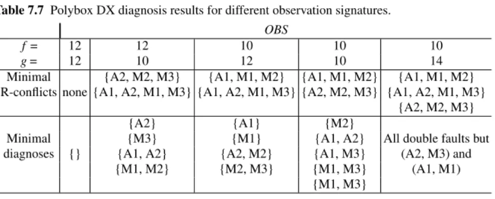
The polybox with the observations as seen above ( f = 10, g = 12) has the fol-lowing minimal R-conflicts: {A1,M1,M2} and {A1,A2,M1,M3} due to the abnor-mal value of 10 for f . Symmetrically, f = 12 and g = 10 yield {A2,M2,M3} and {A1,A2,M1,M3}. In the case f = 10 and g = 10, the two minimal R-conflicts are: {A1,M1,M2} and {A2,M2,M3}. In the case f = 10 and g = 14, the three minimal R-conflicts are: {A2,M2,M3}, {A1,M1,M2}, and {A1,A2,M1,M3}.

The corresponding minimal diagnoses are presented in Table7.7.

7.4.1.3 Bridge

Releasing the exoneration assumption in the polybox example leads to the single fault signature matrix shown in Table7.8and to the extended fault signature matrix

(21)

Table 7.7 Polybox DX diagnosis results for different observation signatures. OBS

f = 12 12 10 10 10

g = 12 10 12 10 14

Minimal {A2, M2, M3} {A1, M1, M2} {A1, M1, M2} {A1, M1, M2} R-conflicts none {A1, A2, M1, M3} {A1, A2, M1, M3} {A2, M2, M3} {A1, A2, M1, M3}

{A2, M2, M3}

{A2} {A1} {M2}

Minimal {M3} {M1} {A1, A2} All double faults but diagnoses {} {A1, A2} {A2, M2} {A1, M3} (A2, M3) and

{M1, M2} {M2, M3} {M1, M3} (A1, M1) {M1, M3}

Table 7.8 Polybox single faults without exoneration. fA1 fA2 fM1 fM2 fM3

ARR1 ⇥ 0 ⇥ ⇥ 0 ARR2 0 ⇥ 0 ⇥ ⇥ ARR3 ⇥ ⇥ ⇥ 0 ⇥ Table 7.9 Polybox double faults signature matrix.

fA1 fA2 fM1 fM2 fM3 fA1A2 fA1M1 fA1M2 fA1M3 fA2M1 fA2M2 fA2M3 fM1M2 fM1M3 fM2M3

ARR1 ⇥ 0 ⇥ ⇥ 0 ⇥ ⇥ ⇥ ⇥ ⇥ ⇥ 0 ⇥ ⇥ ⇥ ARR2 0 ⇥ 0 ⇥ ⇥ ⇥ 0 ⇥ ⇥ ⇥ ⇥ ⇥ ⇥ ⇥ ⇥ ARR3 ⇥ ⇥ ⇥ 0 ⇥ ⇥ ⇥ ⇥ ⇥ ⇥ ⇥ ⇥ ⇥ ⇥ ⇥

presented in Table7.9. These are obtained from the standard ones (see Table7.4and and7.5) by replacing 1’s by ⇥’s, which allows these entries to be matched with 0 or 1 in the observed signature. Note that all signatures of triple faults and more are equal to (⇥,⇥,⇥)T_).

The following results are then obtained:

• With outputs f = 12 and g = 10, i.e. observed signature (0,1,1), there are 4 mini-mal diagnoses: 2 single fault diagnoses {A2} and {M3} and 2 double fault diag-noses {A1, A2} and {M1, M1}, and 22 superset diagdiag-noses.

• With outputs f = 10 and g = 12, i.e. observed signature (1,0,1), there are 4 mini-mal diagnoses: 2 single fault diagnoses {A1} and {M1} and 2 double fault diag-noses {A2, M2} and {M2, M3}, and 22 superset diagdiag-noses.

• With outputs f = 10 and g = 10, i.e. observed signature (1,1,0), there are 5 min-imal diagnoses: one single fault diagnosis {M2} and 4 double fault diagnoses {A1, A2}, {A1, M3}, {M1, A2} and {M1, M3}, and 20 superset diagnoses. • With outputs f = 10 and g = 14, i.e. observed signature (1,1,1), there are 8

min-imal double fault diagnoses: {A1, A2}, {A1, M2}, {A1, M3}, {A2, M1}, {A2, M2}, {M1, M2}, {M1, M3} and {M2, M3}, and 16 superset diagnoses.

These results obtained by FDI are identical to those obtained by DX (see Ta-ble7.7). In the case where f = 12 and g = 12, i.e. observed signature (0,0,0), the empty subset is a minimal diagnosis according to DX and any non empty subset of

(22)

components is a diagnosis according to both approaches: there are 5 minimal single fault diagnoses and 26 superset diagnoses. The only difference between FDI and DX is that, the "no-fault" column of signature (0,0,0) which would correspond to the empty diagnosis subset is left implicit in the signature matrix.

It can be noticed that, except in the f = 10 and g = 14 case (where anyhow, no exoneration can apply as no ARR is satisfied), the results are different from those obtained under the default exoneration assumption (see Table7.6).

7.4.2 Three-tanks case study

For this case study, we use the FDI approach to derive ARRs, then apply the Bridge result to obtain the DX counterpart results.

The system (cf.2.2) is made up of three identical tanks T1,T2,T3. All three tanks have the same physical features such as height and cross sectional area, A. There is a measured input flow qi for tank T1, which is drained into T2via a pipe q12. A similar process gets the flow from T2to T3via pipe q23. Finally, there is an output flow q30from T3. The system has three sensors measuring the level in thanks T1and T3(level transducers LT 1 and LT 2, respectively), and another sensor measuring the flow through pipe q23(flow transducer FT 1).

Adopting the FDI approach, the following three dynamic system equations model the normal behavior of the system. The change in the level in each tank, ˙hT_i, is computed according to mass balances:

e1n: ˙hT₁= qi- q12 A , e2n: ˙hT₂= q12- q23 A , e3n: ˙hT₃= q23- q30 A . Flows between tanks q12,q23,q30are modeled as:

e4n: q12= Sp₁· sign(hT1- hT2) · q 2g | hT1- hT2|, e6n: q23= Sp₂_{· sign(h}T₂- hT₃) · q 2g | hT2- hT3|, e8n: q30= Sp₃_·q2g · hT3,

being Sp_i, i = 1,...,3, the cross sectional area of the pipes. The relation between the state variables, hT_i, and their derivatives ˙hT_iare given by:

e13 : hT₁= ˆ

(23)

e14 : hT₂=ˆ ˙hT₂_{· dt,}

e15 : hT₃= ˆ

˙hT₃_{· dt.}

The above nine equations form the behavioral model BM.

The observational model OM is given by the following equations: e10 : hT₁,obs= hT1,

e11 : hT₃,obs= hT₃, e12 : q23,obs= q23.

Six possible faults are considered: three tank leakages and three pipe blockages as presented in Section2.2.

To obtain ARRs, we can use the structural analysis approach as presented in Section3.4.3or the possible conflicts approach as presented in Section6.1.1. Three ARRs are obtained from the three equation sets below:

{ (e3n)(e8n)(e11)(e12)(e15) }, { (e2n) (e4n) (e6n)(e10) (e11)(e12) (e14)}, {(e1n) (e4n) (e6n) (e10) (e11)(e12) (e13)}.

The fault signature matrix with and without exoneration are given in Table7.10and in Table7.11respectively, where fT_i represents a leakage at the bottom of tank Ti, i = 1,...,3, and fP_jk represents a stuck closed fault on the pipe connecting tank Tj and tank Tkor the atmosphere, i = 1,...,3, k 2 {2,3,0}.

Table 7.10 Three tanks fault signature matrix.

fT1 fT2 fT3 fP12 fP23 fP30

ARR1 0 0 1 0 0 1 ARR2 0 1 0 1 1 0 ARR3 1 0 0 1 1 0

Table 7.11 Three tanks fault signature matrix without exoneration. fT1 fT2 fT3 fP12 fP23 fP30

ARR1 0 0 ⇥ 0 0 ⇥ ARR2 0 ⇥ 0 ⇥ ⇥ 0 ARR3 ⇥ 0 0 ⇥ ⇥ 0

Assume that the observed signature is (0,0,1)T _{then by item 1 of Proposition}_7.1_, we know that {T1,P12,P30_{} is an R-conflict.}

If we use the standard FDI approach and the fault signature matrix of Table7.10, fT₁ is the only fault signature that can be matched. So we get one unique diagnosis

(24)

On the other hand, the DX approach can obtain the diagnoses as the hitting sets of the R-conflicts [19]. In this case, we have one single R-conflict {T1,P12,P30}, which indicates that three minimal diagnoses are 1= {T1}, 2= {P12}, and 3= {P30}. This result seems in contradiction with the result obtained with the standard FDI approach. However, let us now apply the FDI approach by relaxing the ARR-exoneration assumption.

If we now use the FDI approach with no ARR-exoneration, the fault signature matrix of Table 7.11must be considered. Given that a "⇥" entry can be matched to "0" or "1" in the observed signature, not only fT₁ but also fP₁₂ and fP₃₀ can be matched. The diagnosis results are hence the same as for the DX approach, exem-plifying Theorem7.1.

Assume now that the observed signature is (1,1,0)T _{then by item 1 of Proposition}

7.1, we know that {T3,P30} and {T2,P12,P23} are R-conflict.

If we use the FDI approach with (cf. Table7.10) or without ARR-exoneration (cf.7.11), no fault signature matches the observed signature.

On the other hand, if we obtain the diagnoses from the two R-conflicts following the DX approach, we obtain six minimal diagnoses 1= {T3,T2}, 2= {T3,P12}, 3= {T3,P23}, 4= {T2,P30}, 5= {P30,P12}, and 6= {P30,P23}. As a matter of fact, all of them are double fault diagnoses. This is the reason why they could not be found with the single fault signature matrix. Interestingly, the DX approach handles single and multiple faults in the same framework while the FDI approach requires to generate the extended fault signature matrix.

7.5 Conclusions

In this chapter, the FDI approach based on ARRs and the DX logical approach have been compared and the hypotheses underlying the two approaches have been clearly stated. The concepts on both sides have been bridged and it has been shown that the two approaches provide the same diagnosis results under some assumptions referring to exoneration. The classical polybox and the three tanks case studies have been used to illustrate the MBD Bridge from which potential synergies are possible. The links and the understanding of the MBD Bridge provide sound ground for merging the best of both worlds and producing ever better diagnosers for real com-plex systems.

References

[1] Adrot, O., Maquin, D., Ragot, J.: Fault detection with model parameter struc-tured uncertainties. In: Proceedings of the European Control Conference, ECC’99. Karlsruhe (1999)

(25)

[2] Armengol, J., Bregon, A., Escobet, T., Gelso, E., Krysander, M., Nyberg, M., Olive, X., Pulido, B., Travé-Massuyès, L.: Minimal Structurally Overdeter-mined sets for residual generation: A comparison of alternative approaches. Proceedings of the 7th IFAC Symposium on Fault Detection, Supervision and Safety of Technical Processes, Safeprocess’09 (2009)

[3] Basseville, M., Nikiforov, I.: Detection of abrupt changes: theory and applica-tion. Citeseer (1993)

[4] Blanke, M., Kinnaert, M., Lunze, J., Staroswiecki, M.: Diagnosis and fault-tolerant control. Springer Verlag (2003)

[5] Chow, E., Willsky, A.: Analytical redundancy and the design of robust failure detection systems. IEEE Transactions on automatic control29(7), 603–614 (1984)

[6] Cordier, M., Dague, P., Lévy, F., Montmain, J., Staroswiecki, M., Travé-Massuyès, L.: Conflicts versus analytical redundancy relations: a comparative analysis of the model based diagnosis approach from the artificial intelligence and automatic control perspectives. IEEE Transactions on Systems, Man, and Cybernetics, Part B34(5), 2163–2177 (2004)

[7] Denis-Vidal, L., Joly-Blanchard, G., Noiret, C.: Some effective approaches to check the identifiability of uncontrolled nonlinear systems. Mathematics and computers in simulation57(1-2), 35–44 (2001)

[8] Dubuisson, B.: Automatique et statistiques pour le diagnostic. Hermes Science Europe Ltd (2001)

[9] Gertler, J.: Analytical redundancy methods in failure detection and isolation. In: Preprints of the IFAC SAFEPROCESS Symposium, pp. 9–21 (1991) [10] Gertler, J.: Fault Detection and Diagnosis in Engineering Systems. Marcel

Deker (1998)

[11] Katsillis, G., Chantler, M.: Can dependency-based diagnosis cope with simul-taneous equations. In: Proceedings of the 8th International Workshop on Prin-ciples of Diagnosis DX-97, pp. 51–59 (1997)

[12] Kleer, J., Mackworth, A., Reiter, R.: Characterizing diagnoses and systems. Artificial Intelligence56(2-3), 197–222 (1992)

[13] Krysander, M., Aslund, J., Nyberg, M.: An efficient algorithm for finding min-imal overconstrained subsystems for model-based diagnosis. IEEE Transac-tions on Systems, Man and Cybernetics, Part A: Systems and Humans38(1), 197–206 (2008)

[14] Loiez, E., Taillibert, P.: Polynomial temporal band sequences for analog di-agnosis. In: Proceedings of the Fifteenth International Joint Conference on Artificial Intelligence IJCAI-97, Nagoya, Japan, August 23-29, 1997, p. 474 (1997)

[15] Patton, R., Chen, J.: A re-examination of the relationship between parity space and observer-based approaches in fault diagnosis. European Journal of Diag-nosis and Safety in Automation1(2), 183–200 (1991)

[16] Patton, R., Frank, P., Clark, R.: Fault diagnosis in dynamic systems. Theory and Applications (1989)

(26)

[17] Pulido, B., Gonzalez, C.: Possible conflicts: A compilation technique for consistency-based diagnosis. IEEE Transactions on Systems, Man, and Cy-bernetics - Part B: CyCy-bernetics34(5), 2192–2206 (2004)

[18] Qiu, Z., Gertler, J.: Robust FDI and Hinfoptimization. In: Proceedings of the 32nd IEEE Conference on Control and Decision CDC’93. San Antonio, Texas (1993)

[19] Reiter, R.: A theory of diagnosis from first principles. Artificial Intelligence 32(1), 57–95 (1987)

[20] Sachenbacher, M., Williams, B.: Diagnosis as semiring-based constraint op-timization. In: Proceedings of the European Conference on Artificial Intelli-gence ECAI’04, vol. 16, p. 873 (2004)

[21] Staroswiecki, M., Comtet-Varga, G.: Analytical redundancy relations for fault detection and isolation in algebraic dynamic systems. Automatica37(5), 687– 699 (2001)

[22] Staroswiecki, M., Declerck, P.: Analytical redundancy in non linear intercon-nected systems by means of structural analysis. In: Proceedings of the IFAC Symposium on Advanced Information Processing in Automatic Control, pp. 51–55 (1989)

[23] Travé-Massuyès, L.: Bridging control and artificial intelligence theories for diagnosis: A survey. Engineering Applications of Artificial Intelligence27, 1–16 (2014)

[24] Venkatasubramanian, V., Rengaswamy, R., Kavuri, S.N.: A review of process fault detection and diagnosis part ii: Qualitative models and search strategies. Computers and Chemical Engineering27(3), 313–326 (2003)

[25] Venkatasubramanian, V., Rengaswamy, R., Kavuri, S.N., Yin, K.: A review of process fault detection and diagnosis part iii: Process history based methods. Computers and Chemical Engineering27(3), 327–346 (2003). DOI 10.1016/ S0098-1354(02)00162-X-a3

[26] Venkatasubramanian, V., Rengaswamy, R., Yin, K., Kavuri, S.N.: A review of process fault detection and diagnosis part i: Quantitative model-based meth-ods. Computers and Chemical Engineering27(3), 293–311 (2003)

[27] Vento, J., Puig, V., Sarrate, R., Travé-Massuyès, L.: Fault detection and iso-lation of hybrid systems using diagnosers that reason on components. IFAC Proceedings Volumes45(20), 1250–1255 (2012)

[28] Washio, T., Motoda, H., Niwa, Y., INSS, I.: Discovering Admissible Model Equations from Observed Data. In: Proceedings of the 16th International Joint Conference on Artificial Intelligence IJCAI’99, vol. 2, pp. 772–779. Citeseer (1999)

[29] Williams, B., Ragno, R.: Conflict-directed A* and its role in model-based em-bedded systems. In: Journal of Discrete Applied Mathematics. Citeseer (2003)

BRIDGE: Matching Model Based Diagnosis from FDI and DX perspectives

HAL Id: hal-03089393

https://hal.laas.fr/hal-03089393

Submitted on 13 Jan 2021

HAL is a multi-disciplinary open access

archive for the deposit and dissemination of

sci-entific research documents, whether they are

pub-lished or not. The documents may come from

teaching and research institutions in France or

abroad, or from public or private research centers.

L’archive ouverte pluridisciplinaire HAL, est

destinée au dépôt et à la diffusion de documents

scientifiques de niveau recherche, publiés ou non,

émanant des établissements d’enseignement et de

recherche français ou étrangers, des laboratoires

publics ou privés.

and DX perspectives

Louise Travé-Massuyès, Teresa Escobet

To cite this version:

Louise Travé-Massuyès, Teresa Escobet. BRIDGE: Matching Model Based Diagnosis from FDI and

DX perspectives. Teresa Escobet; Anibal Bregon; Belarmino Pulido; Vicenç Puig. Fault Diagnosis

of Dynamic Systems. Quantitative and Qualitative Approaches, Springer International Publishing,

pp.153-175, 2019, 978-3-030-17727-0. �10.1007/978-3-030-17728-7_7�. �hal-03089393�

Fault Diagnosis

of Dynamic Systems

Teresa Escobet

Anibal Bregon

Belarmino Pulido

Vicenç Puig

January 16, 2019

Contents

BRIDGE: Matching Model Based Diagnosis

from FDI and DX perspectives

7.1 Introduction

7.2 DX and FDI MBD approaches

7.2.1 Brief overview of the FDI approach

7.2.2 Brief overview of the DX logical diagnosis theory

7.2.3 Modeling comparison

7.3 DX and FDI model-based diagnosis Bridge

7.3.1 ARR vs. R-conflict

7.3.2 Redundant ARRs

7.3.3 Exoneration assumptions

7.3.4 Comparison in practice

7.4 Case studies

7.4.1 Polybox case study

7.4.2 Three-tanks case study

7.5 Conclusions

References