HAL Id: tel-02864762
https://tel.archives-ouvertes.fr/tel-02864762
Submitted on 11 Jun 2020
HAL is a multi-disciplinary open access
archive for the deposit and dissemination of sci-entific research documents, whether they are pub-lished or not. The documents may come from teaching and research institutions in France or abroad, or from public or private research centers.
L’archive ouverte pluridisciplinaire HAL, est destinée au dépôt et à la diffusion de documents scientifiques de niveau recherche, publiés ou non, émanant des établissements d’enseignement et de recherche français ou étrangers, des laboratoires publics ou privés.
Study of Volatile Organic Compounds (VOC) in the
cloudy atmosphere : air/droplet partitioning of VOC
Miao Wang
To cite this version:
Miao Wang. Study of Volatile Organic Compounds (VOC) in the cloudy atmosphere : air/droplet partitioning of VOC. Earth Sciences. Université Clermont Auvergne, 2019. English. �NNT : 2019CLFAC080�. �tel-02864762�
UNIVERSITE CLERMONT AUVERGNE
DOCTORAL SCHOOL OF FUNDAMENTAL
SCIENCES
PhD Thesis
in partial fulfilment of the requirements for the degree of
Doctor of University Clermont Auvergne
Specialty : Physics-Chemistry of the Atmosphere and Climate
Submitted and presented by
« WANG Miao »
Graduate of the Master Physics and Chemistry for the Environment
Study of Volatile Organic Compounds (VOC) in the cloudy
atmosphere : air/droplet partitioning of VOC
To be defended the 16
thof December 2019
Jury member of the committee:
Huret Nathalie
President
Leriche Maud
Reviewer
Sauvage Stéphane
Reviewer
Mailhot Gilles
Examiner
Beekmann Matthias
Examiner
Colomb Aurélie
Invited
Borbon Agnès
Co-supervisor
UNIVERSITE CLERMONT AUVERGNE
ECOLE DOCTORALE DES SCIENCES
FONDAMENTALES
THESE
présentée pour obtenir le grade de
DOCTEUR D’UNIVERSITE CLERMONT AUVERGNE
Spécialité : Physique-chimie de l’atmosphère et climat
Par « WANG Miao »
Diplômée du Master Physique et Chimie pour l’Environnement
Etude des Composés Organiques Volatils (COV) dans
l’atmosphère nuageuse au sommet du puy de Dôme :
partition air/goutte des COV et impact sur la chimie
atmosphérique
Soutenance prévue publiquement le 16 Décembre 2019 devant le jury :
Huret Nathalie
Président
Leriche Maud
Rapporteur
Sauvage Stéphane
Rapporteur
Mailhot Gilles
Examinateur
Beekmann Matthias
Examinateur
Colomb Aurélie
Invitée
Borbon Agnès
Co-directrice de thèse
Table of contents
Table of contents ... 1
Table of figures ... 4
Table of tables ... 12
Introduction ... 15
CHAPTER I Atmospheric VOC: sources & multiphasic transformations ... 18
General physical and chemical properties of Volatile Organic Compounds (VOC) ... 19
Definition ... 19
Chemical VOC diversity ... 20
Sources of VOC into the atmosphere ... 23
Natural emissions ... 24
I.2.1.1 Plant emissions ... 24
I.2.1.2 Soil emissions ... 25
I.2.1.3 Ocean emissions ... 26
I.2.1.4 Variability of natural emissions from terrestrial ecosystems ... 27
Anthropogenic emissions ... 31
I.2.2.1 Biomass burning ... 31
I.2.2.2 Other anthropogenic emissions ... 33
I.2.2.3 Temporal and spatial variability of anthropogenic emissions... 36
VOC transformations in the atmosphere ... 39
VOC chemical transformations: lifetime estimation ... 39
I.3.1.1 Hydroxyl radicals HO•... 40
I.3.1.2 Nitrate radicals NO3• ... 40
I.3.1.3 Ozone O3 ... 41
VOC reactivity ... 43
I.3.2.1 VOC oxidation ... 43
I.3.2.2 VOC oxidation by ozonolysis ... 44
I.3.2.3 VOC photolysis... 46
I.3.2.4 Comparison of VOC oxidation mechanisms ... 47
Transfer from the gas phase to the particulate phase ... 48
Gas to particle partitioning theory ... 48
SOA precursors ... 49
Parameters influencing SOA formation ... 49
Global SOA production estimates ... 51
Transfer to the aqueous phase ... 53
Henry's Law equilibrium ... 54
Mass transfer: a kinetical process ... 59
Evaluation of gas/liquid partitioning ... 63
Transformations in the aqueous phase ... 65
Abiotic transformations ... 65
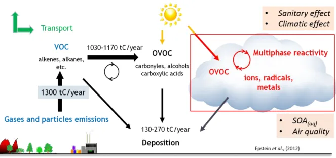
Objectives of the thesis: effect of clouds on the atmospheric VOC budget? ... 67
CHAPTER II Analytical developments for quantification of multiphasic VOC/OVOC in cloud .. 70
Framework of the analytical developments ... 71
Which target compounds? ... 71
Which expertise at LaMP? ... 73
Derivatization techniques for OVOC measurement by GC-MS ... 75
Design of the analytical set-up for VOC/OVOC measurement in gas and cloud phases .. ... 78
Identification and separation of the derivatized OVOC ... 79
Preparation of the derivatized standards ... 79
Identification and separation of carbonyl compounds ... 80
Identification and separation of alcohols and carboxylic acids ... 83
Analysis of carbonyls in the gas phase ... 87
Preamble ... 87
Sorbent coating and derivatization ... 88
Humidity influence ... 89
Derivatization efficiency: liquid derivatization versus on sorbent tube derivatization 90 Linearity of the method ... 91
Time of storage ... 92
The breakthrough volume (BV) ... 93
II.3.7.1 Preliminary tests for ambient air ... 93
II.3.7.2 2,4-dinitrophenylhydrazine (DNPH) sorbent tubes: an alternative for the future? . ... 94
Preliminary analysis of alcohol and carboxylic acid functions using derivatization ... 96
Conclusion for measurement of gaseous carbonyls and perspectives ... 97
Extraction and analysis of VOC and OVOC in the cloud droplet phase ... 98
SBSE: a well-adapted extraction technique for VOC and OVOC in the cloud water and compatible with TD-GC-MS ... 98
SBSE steps ... 99
II.4.2.1 Extraction step ... 99
II.4.2.2 Desorption step ... 100
II.4.2.3 SBSE with derivatization... 101
Optimization of SBSE conditions for VOC extraction ... 102
II.4.3.1 SBSE theory ... 102
II.4.3.2 SBSE optimization ... 103
Optimization of SBSE conditions for the analysis and extraction of OVOC ... 111
II.4.4.1 Carbonyl functions derivatization in liquid phase samples ... 111
Detection limits for OVOC by Tenax® tube and SBSE ... 113
VOC measurement uncertainty ... 114
Summary of the analytical developments ... 119
CHAPTER IIIMultiphasic VOC sampling in the cloudy atmosphere: towards air-water partitioning ... 122
Measurement sites and multiphasic sampling ... 123
Presentation of the puy de Dôme station ... 123
Presentation of the Maïdo observatory ... 124
Multiphasic sampling ... 126
VOC distribution at PUY ... 128
Seasonal variation of VOC at PUY ... 129
Investigation of the influence of the FT/BL alternation on the VOC distribution at PUY ... 130
Comparison of VOC concentrations at PUY with other GAW sites ... 133
Evaluation of air/droplet partitioning for VOC at PUY ... 136
Cloud and gaseous sampling ... 137
History of the air masses: classification of sampled clouds ... 138
Quantification of VOC in gas and liquid phases ... 140
Calculation of the partitioning coefficient “𝑞” ... 143
Discussions about the deviations from the Henry’s law equilibrium ... 149
Preliminary result of VOC and OVOC characterization during the BIOMAIDO campaign .... ... 157
Presentation of the field campaign ... 157
VOC atmospheric concentration during cloud events ... 159
Summary conclusion and perspectives... 163
References ... 165
Table of figures
Figure I-1 Example of vapor pressure of organic compounds at different temperatures. Normal boiling points are represented with black dots; the vapor pressure curve intersects the horizontal
pressure line at 1 atm of absolute vapor pressure
(https://chem.libretexts.org/Bookshelves/Physical_and_Theoretical_Chemistry_Textbook_M aps/Supplemental_Modules_(Physical_and_Theoretical_Chemistry)/Physical_Properties_of_ Matter/States_of_Matter/Properties_of_Liquids/Vapor_Pressure). ... 20 Figure I-2 Anatomy of a eudicot leaf (https://plantstomata.wordpress.com/) (eudicot: clade of flowering plants). ... 27 Figure I-3 Dependence of BVOC emissions on temperature in K (left) and light (right) by PAR (photosynthetically active radiation) in µmol m-2 h-2. Adapted from Steiner and Goldstein
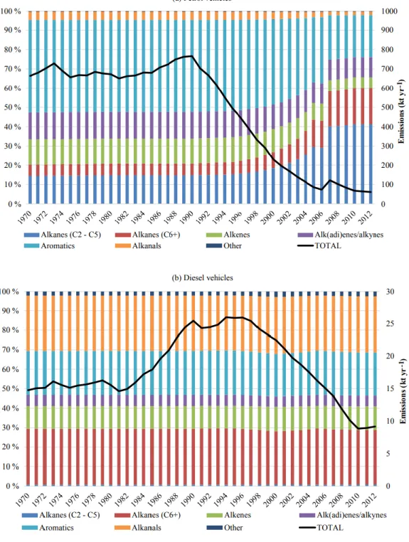
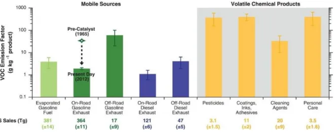
(2007). ... 28 Figure I-4 Isoprene fluxes at the forest site (PROPHET), Michigan during the 2001 growing season. Green and black lines denote MEGAN and measured isoprene fluxes, respectively. Red circles denote isoprene fluxes retrieved from a 6-year (1996–2001) formaldehyde (HCHO) column data set from the Global Ozone Monitoring Experiment (GOME) satellite instrument. Horizontal dashed lines denote uncertainty in the retrieved HCHO vertical columns (Palmer et al., 2006). ... 29 Figure I-5 Representation of VOC emissions linked with biotic interactions in soils. VOC in the soil (blue arrows) are emitted by bacteria (mVOC), fungi (fVOC), roots (rVOC) and litter (lVOC). Direct negative effects (e.g., growth inhibition, toxicity) of VOC are indicated by red arrows; direct and indirect positive effects are indicated by green arrows (Peñuelas et al., 2014). ... 30 Figure I-6 Total anthropogenic VOC combustion emissions and their speciation for (a) petrol vehicles and (b) diesel vehicles of the road transport sector in the UK during 1970–2012 (Huang et al., 2017). ... 34 Figure I-7 Total VOC emission factors with distinction between mobile sources (left) and volatile chemical products (right). The green symbol and dashed arrow illustrate the large reductions in tailpipe VOC emission factors as precatalyst on-road gasoline vehicles were replaced by present-day vehicle fleets (McDonald et al., 2018). Error bars reflect the 95% confidence interval of the mean or expert judgment. ... 35 Figure I-8 (a) The diurnal profile of ambient VOC from whole gasoline and gasoline vapor emissions (Gentner et al., 2009); (b) the seasonal change in the composition of the urban VOC (Boynard et al., 2014). ... 37
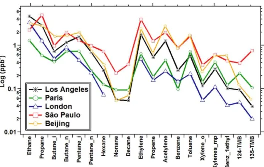
Figure I-9 VOC average mixing ratios in megacities (Dominutti et al., 2016). VOC average mixing ratios have been followed in several megacities such as in São Paulo (Brazil), Beijing (China), London (United-Kingdom), Los Angeles (USA) and Paris (France) in the frame of international projects. ... 38 Figure I-10 Comparison of VOC distribution considered in two different inventories (EDGAR and RETRO)
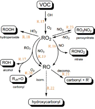
and for two distinct sectors by: Residential combustion and Road transport. EDGAR (E) and RETRO (R) data sets are indicated for Europe (EU), China (CN), and the United States (US) in 2000 (Huang et al., 2017). ... 38 Figure I-11 Simplified pathways for the oxidation of VOC by the radical 𝐻𝑂· in the gas phase from Hallquist et al. (2009). ... 44 Figure I-12 Potential fates of the Criegee intermediate (from Alam et al., 2013). ... 46 Figure I-13 Global budgets (sources/sinks Tg yr−1 and burden Tg) of condensable secondary organic gas
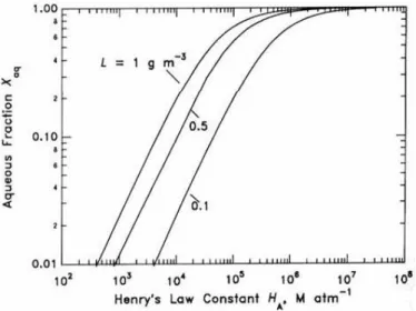
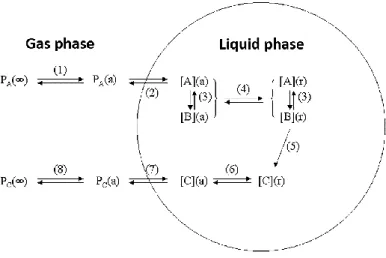
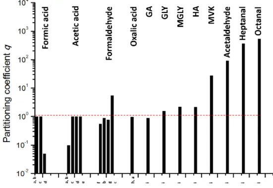
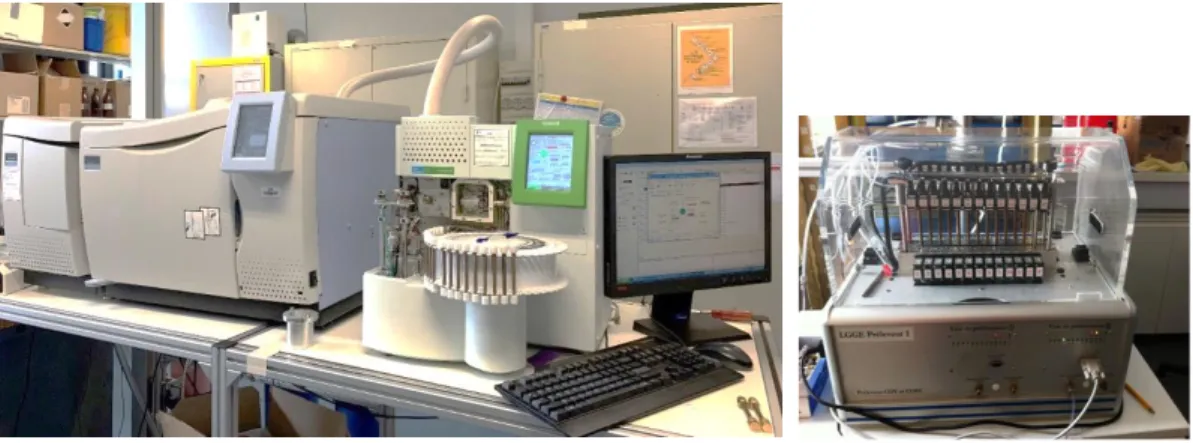
and particle compounds as predicted by GEOS-Chem simulations for 2005–2008 from Hodzic et al. (2016). ... 52 Figure I-14 Effective Henry’s Law Constant for organic acids as a function of pH at a temperature of 278 K. The solid line represents the theoretical effective Henry’s Law constant, while the symbols represent the experimental results obtained from gas and liquid phase measurements (1-h time basis). The error bars account for sampling and analytical errors from Facchini et al. (1992). ... 57 Figure I-15 Aqueous fraction of a chemical species X as a function of the cloud water content (noted as “L” on the figure) and the Henry’s law constant at 298 K (Seinfeld and Pandis, 2016). ... 58 Figure I-16 Schematic of transport and reactive processes which determine the net uptake in gas−liquid interactions (from Davidovits et al., 2006). ... 59 Figure I-17 Physical and chemical processes driving the mass transfer of species A between the gas phase and the liquid phase (adapted from Schwartz, 1986). ... 61 Figure I-18 Observed q values for various species at different locations in cloud/fog conditions (a–i: Winiwarter et al., 1994; Munger et al., 1995; Facchini et al., 1992; Voisin et al., 2000; Keene et al., 1995; Ricci et al., 1998; Li et al., 2008; Sellegri et al., 2003; van Pinxteren et al., 2005). GA: glycolaldehyde; GLY: glyoxal; HA: hydroxyacetone; MVK: methyl vinyl ketone. ... 64 Figure I-19 Scientific context: VOC in the atmosphere and their climate and sanitary effects. ... 68 Figure I-20 VOC multiphase chemistry: reactivity and air/droplet exchanges. ... 69 Figure II-1 The analytical TD-GC-MS system available at LaMP (left) and the automatic sampling module-SASS (Smart Automatic Sampling System) installed et the puy de Dôme station (right). ... 75
Figure II-2 Derivatization reaction of carbonyl compounds -C=O by the O-(2,3,4,5,6 pentafluorobenzylhydroxylamine (PFBHA) reagent. ... 76 Figure II-3 Derivatization reaction of carboxyl or hydroxyl compounds -OH by the
N-Methyl-N-(t-butyldimethylsilyl)trifluoroacetamide (MTBSTFA) reagent... 77 Figure II-4 Steps (in bold characters) of the analytical developments addressed during my PhD thesis. The measurement of VOC on Tenax TA tubes was already handled. ... 78 Figure II-5 Chromatogram of carbonyl compound standards prepared and derivatized with PFBHA (extracted by m/z 181 from total SIM ion chromatogram). Peak identification is noted with corresponding compound by red arrow. HCHO: formaldehyde; MACR: methacrolein; MVK: methyl vinyl ketone; HA: hydroxyacetone; GLY: glyoxal; MGLY: methylglyoxal. ... 82 Figure II-6 Chromatogram of methanol derivatized with MTBSTFA from total SIM ion chromatogram. Peak identification is noted with red arrow and its mass spectrum. ... 85 Figure II-7 Chromatogram of glycolic acid derivatized with MTBSTFA from total SIM ion chromatogram. Peak identification is noted with red arrow and its mass spectrum. ... 86 Figure II-8 Calculated breakthrough volumes (BV) at 20 °C and for 250 mg of Tenax tubes for C1–C8 carbonyls and alcohols (red triangles). The air sampling volumes (dotted lines) of 6 L and 12 L correspond, respectively, to a sampling duration of 40 min and 120 min at a flow rate of 100 mL min-1. Source: https://www.sisweb.com/index/referenc/tenaxta.htm#aldehydes. The BV
exponentially decreases with temperature. The red full line corresponds to a sampling volume of 0.5 L i.e., 5 min sampling at a flow rate of 100 mL min-1. ... 88
Figure II-9 Laboratory set-upfor the PFBHA coating process on Tenax® tubes. A controlled nitrogen flow at 100 ml min−1 tube−1 passes through the glass bulb that contains solid PFBHA powder
connected to 8 Tenax® sorbent tubes. ... 89 Figure II-10 Design of the humid air generating system. ... 89 Figure II-11 Humidity influence (0% RH, 50% RH and 90% RH) of derivatized carbonyl compounds
on-Tenax tube. “Peak area” refers to the 181 m/z with chromatogram obtained in the electron ionization mode, in area units. Error bars represent ± one standard deviation determined from 5 triplicates. ... 90 Figure II-12 Comparison of responses for in-solution and on-sorbent-tube PFBHA derivatization of carbonyls: “Peak area” refers to chromatogram with 181 m/z, in area units. Error bars represent ± standard deviation determined from repeatability tests. Both in-solution and on-sorbent-tube derivatization were performed more than four times. ... 91
Figure II-13 Calibration curves of methacrolein (MACR) and butanal after derivatization on Tenax® tube pre-coated with PFBHA. “Peak area” refers to chromatogram with 181 m/z, in area units. ... 92 Figure II-14 Influence of storage time from five days to twenty three days. Relative response refers to a ratio between peak area of a derivative compound and the one of pentanal (in order to show these compounds in the same figure clearly)... 93 Figure II-15 First evaluation of the breakthrough volume of some aldehydes. Dark color: signal in the front tube. Light color: signal in the back tubes (when observed, value in % of the signal on the sampling tube). a) Testing formaldehyde BV for different air volume sampling; b) testing BV of some C4−C5 carbonyl for a 6 L-air volume sampling. Note that for the a) case, each BV test is carried out under different sampling concentrations. ... 94 Figure II-16 Laboratory system of adjustable gaseous flow of carbonyl compounds controlled by a supplementary RH system at SAGE IMT Lille Douai and a picture of the combined system. . 95 Figure II-17 The calibration curves at 50 and 90% RH for MVK and MACR using DNPH tubes analysed by HPLC. ... 96 Figure II-18 External calibration curves for methanol and pyruvic acid on MTBSFA pre-coated tubes. “Peak area” refers to chromatogram with their characteristic ions m/z, in area units. ... 97 Figure II-19 A Twister Kit of SBSE. ... 99 Figure II-20 Extraction step with modes in SBSE: immersion (a) and headspace (b) (from Prieto et al., 2009). ... 100 Figure II-21 Different derivatization modes in SBSE: in situ (a), on-stir-bar with the derivatization reagent preloaded before exposure to the sample (b) and in-tube derivatization (from Prieto et al.,2009). ... 101 Figure II-22 Example of theoretical extraction efficiency for 5, 10 and 20 mL sample volumes and 24, 47, 63, 126 µL PDMS volumes. ... 103 Figure II-23 Test of SBSE optimization. ... 103 Figure II-24 Effects of PDMS volume (A), extraction time (B), sample volume (C) and NaCl effect (D) on the extraction efficiency E (%) for a selection of VOC:dichloromethane, benzene, toluene, 1,1,2-trichloroethane, ethylbenzene, m-xylene, p-xylene, styrene, o-xylene, 1,3,5-trimethylbenzene, 1,2,4-1,3,5-trimethylbenzene, 1,2,3-trichlorobenzene and n-butylbenzene. . 106 Figure II-25 Effects of NaCl addition on the extraction efficiency E (%) for a all standards of VOC, classified ranging from low log Ko/w = 1.18 to high log Ko/w = 4.72. ... 107
Figure II-26 Example of theoretical extraction efficiency for 5, 10 and 20 mL sample volumes and 63, 126 µL PDMS volumes and comparison between experimental and theoretical extraction
efficiency with experimental conditions based on 63 µL PDMS volume and 5 mL sample
volume. ... 108
Figure II-27 Calibration curves for toluene and isoprene for external (red) and internal (blue) calibration. “Peak area” refers to the total ion chromatogram obtained in the electron ionization mode, in area units. ... 110
Figure II-28 Chromatogram of VOC (from total SIM ion chromatogram) extracted by SBSE. Peak identification is noted with corresponding compound by red arrow. ... 110
Figure II-29 Effects of extraction time (3 h, 4 h and 6 h) and NaCl effect (with the presence of NaCl in black and without the presence of NaCl in red) on the extraction for MVK and butanal. “Peak Area” refers to the m/z 181 extracted ion chromatogram obtained in the electron ionization mode, in area units. ... 112
Figure II-30 The external (red) and internal (blue) calibration curves for MACR and pentanal. “Peak Area” refers to the m/z 181 extracted ion chromatogram obtained in the electron ionization mode, in area units. ... 113
Figure II-31 Chromatogram of carbonyl compounds, derivatized with PFBHA (extracted by m/z 181 from total SIM ion chromatogram) and extracted by SBSE. Peak identification is noted with corresponding compound by red arrow. HCHO: formaldehyde; MACR: methacrolein; MVK: methyl vinyl ketone; GLY: glyoxal; MGLY: methylglyoxal. ... 113
Figure II-32 Observational strategy overview. ... 119
Figure III-1 Overview maps showing the location of CO-PDD sites as well as photography of the different sites and altitudes. This picture is extracted from Baray et al. (2019). ... 124
Figure III-2 Localization of Maïdo observatory and a picture of the building. ... 125
Figure III-3 One-stage cloud water impactors of LaMP. ... 126
Figure III-4 The new cloud water collector of LaMP. ... 127
Figure III-5 New system for simultaneous sampling in both gas and liquid phases. ... 127
Figure III-6 Presentation of the instruments deployed during the BIOMAIDO field campaign in 2019 for collecting gaseous compounds and cloud droplets. ... 128
Figure III-7 Distribution of major gaseous VOC concentrations (ppbv) during 2010-2013 at PUY station. The number of samples analyzed is indicated under each box plot. The bottom and top of box plots are the 25th and 75th percentiles, respectively. The full line and the open square symbol represent the median and mean values, respectively. The “-” represents 10th and 90th percentiles. ... 129 Figure III-8 Distribution of VOC concentrations (ppbv) in summer (red boxplots) and in winter (blue boxplots) 2012 and 2013 at PUY station. The number of samples analyzed is indicated under
each box plot. The bottom and top of box plots are the 25th and 75th percentiles, respectively.
The full line and the open square symbol represent the median and mean values, respectively. The “-” represents 10th and 90th percentiles. ... 130 Figure III-9 Evolution of the boundary layer height as a function of the time (shown with local time in hour) during the July of 2015. ... 131 Figure III-10 Distribution of a selection of VOC in the free troposphere (FT) and in the boundary layer (BL) (from the thesis of A. Farah, 2018). ... 131 Figure III-11 Diurnal evolution of isoprene concentration (in green) at PUY in July 2015 along with ambient temperature (in red) and boundary layer (BL) height (in grey). ... 132 Figure III-12 Scatterplot of toluene to benzene concentrations in winter (blue dots) and in summer (red dots) from VOC data collected between 2010 and 2015 at PUY station. The urban emission ratios (ER) are the ones provided by Schnitzhofer et al. (2008) in a highway tunnel in Europe. ... 133 Figure III-13 Location of other Global Atmosphere Watch program sites: Mt. Cimone station (CMN) in green frame, Hohenpeißenberg station (HPB) in yellow frame and PUY station in pink frame. ... 134 Figure III-14 Distribution of VOC concentrations (ppbv) for 2010-2013 measured at PUY station (pink boxplots), HPB station HPB station (green boxplots) and CMN (yellow boxplots). The number of samples analyzed is indicated under each box plot. The bottom and top of box plots are the 25th and 75th percentiles, respectively. The full line and the open square symbol represent the
median and mean values, respectively. The “-” represents 10th and 90th percentiles. ... 134
Figure III-15 Seasonal distribution of VOC concentrations (ppbv) in summer June and July (red boxplots) and in winter January and February (blue boxplots) 2012 and 2013 at PUY (A) and HPB (B) for VOC. The number of samples analyzed is indicated under each box plot. The bottom and top of box plots are the 25th and 75th percentiles, respectively. The full line and the open square
symbol represent the median and mean values, respectively. The “-” represents 10th and 90th
percentiles. ... 135 Figure III-16 Seasonal distribution of VOC concentrations (ppbv) in summer June and July (red boxplots)
and in winter January and February (blue boxplots) 2012 and 2013 at PUY (A) and CMN (B) for VOC... 136 Figure III-17 Distribution of VOC concentrations (ng mL−1) in cloud waters sampled at PUY station for
VOC from anthropogenic sources (black boxplots) and from biogenic origin (green boxplots). The number of samples analyzed is indicated above each box plot. The bottom and top of box plots are the 25th and 75th percentiles, respectively. The full line and the open square symbol
represent the median and mean values, respectively. The ends of whiskers are 10th and 90th percentiles. The asterisks are maximum and minimum values. Note that 1,3,5-TMB, 1,2,4-TMB, 1,2,3-TMB stand for 1,3,5-trimethylbenzene, 1,2,4-trimethylbenzene and 1,2,3- trimethylbenzene. ... 141 Figure III-18 Concentration variability of VOC in gas phase in ppbv (in orange) and in cloud water samples in ng mL-1 (in blue) during parallel sampling periods of 2014 at PUY station (clouds
number C5 S1, C8 S2, C9 S1, C9 S2 and C9 S3). The top and bottom of line are maximum and minimum values. The square and asterisk symbols represent the mean values of VOC in gas phase and in cloud water samples, respectively. ... 143 Figure III-19 q factors calculated for each cloud sample and for each chemical compound (blue circles correspond to mean values). ... 148 Figure III-20 Mean q factors calculated in this study are compared with the study from van Pinxteren et al. (2005); chemical compounds are classified as a function of their effective Henry’s law constants. ... 148 Figure III-21 (A) Enrichment factors E for each chemical compound and for each cloud sample presenting different mean droplet radius rmean and concentrations of non-dissolved organic
carbon (𝜌𝑠 ∗). For C9 cloud event, is presented the E coefficient averaged for the 3 samples (mean radius and mean non-dissolved organic carbon); (B) Enrichment factors E for each chemical compound of samples from cloud event C9 with mean droplet radius rmean for
samples and different concentrations of non-soluble organic compounds... 151 Figure III-22 𝐾𝑜𝑐 as a function of 𝐾𝑜/𝑤 (left); air-water interfacial binding constant 𝐾𝑎 as a function of 𝐾𝑜/𝑤 (right) (from Valsaraj et al., 1993). ... 152 Figure III-23 Enrichment factor as a function of Koc and Ka. Note that for 𝑟=10 µm and 𝜌𝑠 ∗=20 mgC L-1
without coloration; for 𝑟=1 µm and 𝜌𝑠 ∗=200 mgC L-1, 𝑟=1 µm and 𝜌𝑠 ∗=20 mgC L-1 with
coloration in red and blue, respectively. ... 155 Figure III-24 Summarize of the various instrumented sites allowing the sample atmospheric compartments along the mountain slope during the BIOMAIDO campaign. ... 157 Figure III-25 Field campaign blanks with sealed and non-sealed tubes. One field campaign blank tube is kept sealed during the whole field campaign “‘Field campaign blank with sealed tube” (red dots). The other field campaign blank is connected to the AEROVOCC device during the sampling without any air flow “Field campaign blank with sealed tube” (black dots). ... 159 Figure III-26 Gaseous mixing ratios of biogenic VOC measured during the cloud events (indicated with “R”). ... 159
Figure III-27 Gaseous mixing ratios of anthropogenic VOC measured during the cloud events (indicated with “R”). ... 160 Figure III-28 Distribution of OVOC mixing ratios (ppbv) during BIOMAIDO for the various cloud events (MVK: methyl vinyl ketone; MGLY: methylglyoxal; GLY: glyoxal). ... 161
Table of tables
Table I-1 Classification of major atmospheric VOC into categories based on their chemical structures
and examples of compounds are given. ... 21
Table I-2 Estimated annual global emissions of major BVOC (based on Fall et al., 1999). ... 24
Table I-3 Global emission of selected species based on the emission factors and the biomass burning estimates (in Tg y-1) (Andreae, 2019). ... 32
Table I-4 Calculated tropospheric lifetimes of selected VOC due to photolysis and reaction with HO• and NO3• radicals and ozone O3 (HO•, 12-hour average concentration of 1.5 106 molec cm-3 (0.06 ppt) (Prinn et al., 1987); NO3• 12-hour average concentration of 5.0 108 molec cm-3 (20 ppt) (Atkinson, 1991); O3 24-hour average concentration of 7.0 1011 molec cm-3 (28 ppb) (Logan, 1985). Calculated from 20 °C rate data of Atkinson (1988, 1990a, 1991), Plum et al. (1983), and Rogers (1990). “/”was expected to be of negligible importance.) (https://www.nap.edu/read/1889/chapter/7#123). ... 42
Table I-5 Modification of the vapor pressure for organic compounds when adding a functional group. The indicated values correspond to a multiplicative factor applied to the vapor pressure of the compound (in atm). The addition of a carbon on the molecular chain is given as an indication. This table is derived from Kroll and Seinfeld (2008). ... 47
Table I-6 Henry’s law constants at 298 K and ∆𝐻 enthalpy variation for a selection of chemical species. ... 55
Table I-7 Characteristic times associated to each steps describing the mass transfer of a species A between the gas phase and cloud droplets... 61
Table II-1 List of target compounds in our study. ... 72
Table II-2 Obtained fragmentation pattern and observed structure for PFBHA... 80
Table II-3 Molecular structure, parent mass weight (MW), derivative MW, GC retention times and characteristic mass of PFBHA derivatives of carbonyl compounds. ... 81
Table II-4 Obtained fragmentation pattern and observed structure for MTBSTFA derivatives. ... 83
Table II-5 Molecular structure, parent mass weight (MW), derivative MW, GC retention times and characteristic mass of MTBSTFA derivatives of hydroxyl compounds. ... 84
Table II-6 Extraction efficiency (E) of SBSE for a selection of VOC (%). ... 109
Table II-7: Detection limits for the analyzed OVOC. ... 114
Table II-8 Calculated uncertainties of VOC concentrations in air and cloud waters. ... 118
Table II-9: Detection limits for the analyzed VOC “*”refers to the calculation for a sampling of 18 L of air (100 ml min-1 for 3h of sampling). ... 118
Table III-1 Comparison of VOC concentrations (min-max, mean value) in gaseous at PUY, HPB and CMN stations (pptv) during 2012 and 2013 (/: below detection limit). ... 136 Table III-2 Cloud sampling dates and durations. C stands for “Cloud events” and S stands for “Samples” collected during one single cloud event. ... 137 Table III-3 Among the 16 cloud samples (presented in next table), five cloud samples present simultaneous air samples. Sampling times (beginning and ending) are indicated for air samples (orange lines) and cloud samples (blue lines). For each air sample, 18L of air has been pumped into the cartridge and is indicated in grey lines. For cloud samples, the volume of air that have been pumped is also indicated and the obtained cloud water volume is indicated as well. 138 Table III-4 Chemical and physical properties of the 9 cloud waters collected at the PUY station. Liquid water content (LWC) is averaged over the sampling period. Note that ND means “not determined” in samples, BDL means “below detection limit”, Mar means “marine” and Cont means “continental”. ... 139 Table III-5 Comparison of VOC concentrations (min-max, mean value) in cloud aqueous phases measured at PUY with similar measurements performed at other sampling sites (/: below detection limit.). ... 142 Table III-6 Comparison of VOC concentrations (min-max, mean value) in gaseous phases measured at PUY with similar measurements performed at other sampling sites (/: below detection limit). ... 144 Table III-7 Summary of all parameters: average measured LWC, experimental concentrations of detected VOC in air (“gas”) and aqueous (“aq”) phases, Henry’s law constant at 298.15K, average in situ temperatures measured during each cloud events, partitioning factors q calculated for each cloud events. ... 145 Table III-8 Cloud droplet radius r (µm) (with min, max and mean values over the collection period) and DOC concentrations (mgC L-1) for each cloud events... 152
Table III-9 Parameters used for the calculation of the enrichment factors E: Octanol-water partition coefficients (Ko/w); cloud droplet radius r (µm) (min, max and mean values) and DOC
concentrations (mgC L-1) for each cloud cloud events. ... 154
Table III-10 The identification of gas and cloud event samplings during BIOMAIDO in 2019, with sampling date, number of cloud event, measurement type of gas, sampling time (local time) and sampling volume of air. Each line in the table corresponds to a cartridge analyzed afterwards. ... 158 Table III-11 VOC concentrations (min-max, mean value) during the cloud events of BIOMAIDO field campaign. ... 160
Introduction
Volatile Organic Compounds (VOC), including saturated, unsaturated, and other substituted
hydrocarbons, play a major role in atmospheric chemistry (Atkinson, 2000). They are primarily emitted by anthropogenic and biogenic sources into the atmosphere; they are also transformed in situ by chemical reactions, and more specifically, by photo-oxidation leading to the formation of ozone (O3)
and Secondary Organic Aerosol (SOA) (Atkinson and Arey, 2003; Kanakidou et al., 2005; Goldstein and Galbally, 2007; Carlton et al., 2009; Hallquist et al., 2009; Chen et al., 2018; Palm et al., 2018). By altering the organic fraction of aerosol particles, VOC modify the Earth’s radiative balance through a direct effect (absorption and scattering of solar radiation) or through indirect effect by altering cloud microphysical properties (Scott et al., 2014). They also present a direct effect on human health and on the environment (Zhu et al., 2018).
During their atmospheric transport, VOC and their oxidation products, Oxygenated Volatile Organic Compounds (OVOC), may partition between the gaseous and aqueous phases depending on their solubility. Clouds have a significant effect on tropospheric chemistry by redistributing trace constituents between phases and by providing liquid water in which aqueous phase chemistry can take place (Herrmann et al., 2015). Indeed, during the cloud lifetime, chemical compounds and particularly VOC are efficiently transformed since clouds favor the development of complex “multiphase chemistry”. The latter presents several particularities. First, photochemical processes inside the droplets are important in the transformation of chemical compounds (Barth, 2006; Vione et al., 2006). Second, aqueous chemical reactions are efficient and can be faster than the equivalent reactions in the gas phase. This can be related to the presence of strong oxidants such as hydrogen peroxide H2O2 or Transition
Metal Ions (TMI), which participate in the formation of radicals such as hydroxyl radicals (HO•) that favor oxidation processes (Deguillaume et al., 2005). Furthermore, the presence of viable microorganisms has been highlighted and shown to participate in transformations of the chemical species (Vaïtilingom et al., 2013; Bianco et al., 2019). Finally, these transformations in clouds are also strongly perturbed by microphysical processes that control formation, lifetime and dissipation of clouds. These processes will redistribute the chemical species between the different reservoirs (cloud water, rain, particle phase, gaseous phase, and solid ice phase) (Marécal et al., 2010; Rose et al., 2018). In this frame, the transformation of VOC in the cloud medium can lead to the production of secondary compounds contributing to SOA formation, reported as “cloud aqSOA” (Ervens, 2015). This secondary organic aerosol mass produced during the cloud lifetime could explain in part the ubiquity of small dicarboxylic and keto acids and high molecular-weight compounds measured in aerosol particles, fog water, cloud water, or rainwater at many locations, as they have neither substantial direct emission sources nor any identified important source in the gas phase. This aqSOA mass stays in the particle phase after cloud evaporation implying a modification of the (micro)physical and chemical properties
of aerosol particles (particle size, chemical composition, morphology). This leads to modifications of their impacts on consecutive cloud or fog cycles (aerosol indirect effects) and of their interactions with incoming radiation by scattering/absorbing (aerosol direct effect).
Measurements of chemical compounds in cloud aqueous phase have been conducted for decades and have been more recently focused on the characterization of the dissolved organic matter (Ervens et al., 2013; Cook et al., 2017; Zhao et al., 2013; Bianco et al., 2018). Among this complex matrix, a significant fraction of organic compounds comes from the gas phase. Indeed, many secondary organic species such as carbonyls and carboxylic acids are formed during the gas phase oxidation of hydrocarbons; since they are highly soluble, they solubilize into the aqueous phase. They also result from aqueous phase processes (chemical and biological transformations). This explains why those compounds have been commonly measured in atmospheric waters (van Pinxteren et al., 2005; Matsumoto et al., 2005; Sorooshian et al., 2006; Deguillaume et al., 2014). However, few studies have
been conducted looking in parallel both compartments (gas and aqueous phases) in order to estimate how VOC compounds are partitioned. This can be partly explained by the inherent
difficulty of sampling clouds. However, this is of major importance since this gives indication of how the cloud is able to scavenge and transform them during their lifetimes.
Using a rough approach, the partitioning of organic compounds between gas and aqueous phases can be described by Henry’s law constants that is to assume thermodynamic equilibrium for all species. However, cloud chemistry models (Lim et al., 2005; Barth, 2006; Ervens, 2015; Rose et al., 2018) and few observational studies (Facchini et al., 1992; Winiwarter et al., 1992; van Pinxteren et al., 2005; Li et al., 2008) have highlighted deviations from the Henry’s law equilibrium. Many factors control the partitioning between these two phases such as the pH, the droplet size, and the reactivity in both phases. Kinetic transport limitations through the droplet surface have to be considered, as they can be perturbed by the presence of hydrophobic molecules at the air/water interface. In this frame, cloud chemistry models simulate the mass transfer between the two phases but those models have to be evaluated towards in situ estimates that are actually scarce (Winiwarter et al., 1994; van Pinxteren et al., 2005).
My thesis work aims at improving the knowledge on the air-water partitioning of VOC in the cloud
multiphasic system. To investigate partitioning, simultaneous air/cloud samplings need to be carried
out. Two classes of VOC have been chosen. First, we decided to focus upon the analysis of VOC of atmospheric interest from anthropogenic and biogenic origin. They include benzene, toluene, ethylbenzene and xylenes (BTEX) as well as biogenic species like isoprene and other terpenes. These compounds are usually detected in the gas phase but are not expected to be present in the aqueous phase due to their low solubility. Beyond the health impact for some of them, like benzene (Cocheo et al., 2000), these compounds are also well-known to contribute to the formation of secondary pollutants like ozone and SOA (Hu et al., 2008; Fu et al., 2009). This first choice was motivated by previous works
that highlighted the accumulation of hydrophobic compounds in the aqueous phase (Valsaraj, 1988a,b; Valsaraj et al., 1993). A second category of VOC of atmospheric interest has been selected for their ability to efficiently dissolve in the aqueous phase due to their high solubility. Those compounds are
OVOC such as carbonyls, carboxylic acids and alcohols. Those compounds are known to be primary
emitted and also produced by homogenous gas phase reactivity and they are suspected to lead to aqSOA mass formation in the aqueous phase.
LaMP has a long experience in the off-line sampling of gaseous VOC on sorbent tubes. VOC samples are analyzed by Gas Chromatograph–Mass Spectrometer system (GC-MS) connected to a Thermal Desorption unit (TD) TD-GC-MS. However the OVOC analysis needed more developments based on a molecular derivatization step before TD-GC-MS analysis. To investigate VOC and OVOC in cloud water, a new extraction method, Stir Bar Sorptive Extraction (SBSE) has been developed. All these developments have been part of my thesis work. Then, two sites presenting different environmental conditions (seasons, origin of air masses, and level of pollution...) have been chosen for testing the new experimental developed devices developed for VOC/OVOC characterization. The puy de Dôme
station has been naturally selected because it offers all the facilities for sampling natural clouds (gas
and aqueous phases) and this station is a reference site for cloud studies (Baray et al., 2019). The second site is La Réunion Island (Pacific Ocean) where a field campaign (BIOMAIDO campaign, ANR program) was performed in spring 2019 for studying the atmospheric organic matter transformation during a cloud cycle. In this frame, VOC and OVOC were sampled and recently quantified by our analytical methods. All those elaborated data will allow to evaluate cloud chemistry models for their ability to reproduce air/water partitioning. In this frame, the new cloud chemistry model CLEPS (Cloud Explicit Physico-Chemical Scheme) developed at LaMP will be used to simulate cloud events on these two sites in the future.
In CHAPTER I, VOC “history” in the atmosphere are presented: sources, transformations and incorporation into the atmospheric condensed phases (particles, cloud). Associated uncertainties to these processes are highlighted since they motivates the goal of my thesis. In CHAPTER II, instrumental developments both in the field and in the laboratory are presented. In the laboratory, new analytical procedures have been developed to quantify VOC and OVOC in both gas and cloud water phases by TD-GC-MS analysis. These developments have been tested on real matrices sampled at the top of the puy de Dôme station (France) and/or at the Maïdo observatory at La Réunion Island). The results are detailed in CHAPTER III.
CHAPTER I
Atmospheric
VOC:
sources
&
multiphasic transformations
General physical and chemical properties of Volatile Organic Compounds (VOC)
Definition
Chemically, a volatile organic compound (VOC) is a compound containing at least one carbon atom together with atoms of hydrogen, oxygen, nitrogen, sulfur, halogens, phosphorous and silicon, excluding carbon monoxide, carbon dioxide, carbonic acid, metallic carbides or carbonates and ammonium carbonate. Hydrocarbons are included but are often mistakenly equated with it. This is probably because VOC are often expressed as total methane- or propane-equivalent hydrocarbons. Methane (CH4), which is a specific VOC and a greenhouse gas naturally widely present in the air, is
often considered apart from the other VOC, which are referred to as non-methane volatile organic compounds (NMVOC). VOC are generally considered as NMVOC.
Physically, VOC are organic chemical compounds whose composition makes it possible for them to evaporate under “normal” atmospheric conditions of temperature and pressure. Following European directives, VOC means “any compound organic having a vapor pressure of 0.01 kPa or more at a temperature of 293.15 K or having a corresponding volatility under the particular conditions of use”. “Volatility” can be quantitatively defined, either by its vapor pressure that is more than 0.01 kPa (European Directive; National Pollutant Inventory (NPI) of Australia www.npi.gov.au), or by its boiling point that is between 50–250 °C (United States Environmental Protection Agency (EPA) www.epa.gzov; Health Canada (HC) www.hc-sc.gc.ca).
The vapor pressure value is used to characterize the tendency of a substance to vaporize. At a given temperature, a substance with a higher vapor pressure will vaporize more readily than a substance with a lower vapor pressure. The vapor pressure of a substance is the pressure at which its gaseous (vapor) phase is in equilibrium with its liquid or solid phase. It is a measure of the tendency of molecules and atoms to escape from a liquid or solid matrix. At atmospheric pressures, when a liquid's vapor pressure increases with increasing temperature to the point at which it equals the atmospheric pressure, the liquid has reached its boiling point, namely, the temperature at which the liquid changes its state to a gas throughout its bulk. That temperature is commonly referred to as the “liquid's normal boiling point”. The higher is the vapor pressure of a liquid, the higher is the volatility and the lower is the normal boiling point of the liquid.
For example, at any given temperature, methyl chloride (CH3Cl) has the highest vapor pressure in
comparison to other VOC in Figure I-1. CH3Cl also has the lowest normal boiling point (-26 °C), which
corresponds to the intercept between its vapor pressure curve (the blue line) and the horizontal pressure line of one atmosphere (atm) of absolute vapor pressure. This compound, widely used as a refrigerant, is therefore very volatile and is emitted in the air.
Figure I-1 Example of vapor pressure of organic compounds at different temperatures. Normal boiling points are represented with black dots; the vapor pressure curve intersects the horizontal pressure line at 1 atm of absolute vapor pressure (https://chem.libretexts.org/Bookshelves/Physical_and_Theoretical_Chemistry_Textbook_Maps/Supplemental_Modules_(P hysical_and_Theoretical_Chemistry)/Physical_Properties_of_Matter/States_of_Matter/Properties_of_Liquids/Vapor_Press ure).
Chemical VOC diversity
VOC are a vast and diverse group of compounds presenting various physical-chemical properties. Physical properties include melting point and boiling point and chemical properties include reactivity and flammability. All of these properties are linked with the chemical structure of the compound. The chemical structure presents high variability with different bonding angles, type of bonds, carbon chain sizes, chemical functions, etc. Changes in the chemical structure drastically affect the properties of the compound. Even isomers, compounds with the same chemical formula but different structures, can have very different properties. Some of main classes of VOC emitted into the atmosphere are presented in
Table I-1 Classification of major atmospheric VOC into categories based on their chemical structures and examples of compounds are given.
Family Selection of VOC compounds with various chemical structure
Hydrocarbons Alkanes, alkenes,
alkynes Propane Ethene 2-butyne Aromatics
Benzene Toluene
o-xylene m-xylene o-xylene
Terpenes Isoprenoids (C5H8)n Hemiterpenoids (n=1, C5H8) Isoprene Monoterpenoids (n=2, C10H16)
α-pinene β-pinene Limonene Sesquiterpenoids (n=3, C15H24) β-Caryophyllene Oxygenated terpenoids Methylchavicol Oxygenated VOC (OVOC) Carbonyl compounds
Formaldehyde Acetaldehyde Acetone
Carboxylic acids
Alcohols
Ethanol Propanol
Others Organic compounds
with heteroatoms (S, N, Cl, Br, ...) Organosulfates Organonitrates Organohalides Pesticides Polychlorinated biphenyls (PCBs) Polycyclic aromatic hydrocarbons (PAHs)
Acetyl chloride Napthalene
Organosulfate Pyrene
Hydrocarbons, more specifically Non-Methane Hydrocarbon Compounds (NMHCs), include several chemical families of species that consist only of carbon and hydrogen atoms: alkanes, alkenes, alkynes and aromatic compounds:
- Alkanes are saturated compounds, consisting of covalent bonds C–C and C–H, and their structures may be linear (e.g., ethane, propane see in Table I-1), branched (e.g., i-butane, 2-methylpentane) or cyclic (e.g., cyclopentane). These compounds are relatively stable and not very reactive. Indeed, it is necessary to provide a substantial energy to dissociate the atoms of a single bond. Carbon–hydrogen bonds have a bond energy of about 483 kJ mol-1 and carbon-carbon of about 347 kJ mol-1.
- Alkenes and alkynes are unsaturated compounds having respectively at least one double or one carbon-carbon triple bond. Unsaturation includes a simple bond (σ-bonding) to which is added one or two bonds of π-bonding. Like the alkanes, they can also be linear (e.g., ethylene, propene and acetylene), branched (e.g., trans-2-pentene) or cyclic (e.g., cyclopentene). At the same number of carbon atoms, the alkenes and the alkynes are more reactive than the alkanes because the energy to be supplied to break their liaison is lower (259 kJ mol-1 to break the first π-bonding of C=C and 226 kJ.mol-1 for the second π-bonding of C≡C).
- Aromatic compounds are cyclic compounds, including in particular benzene, toluene, xylenes and trimethylbenzenes (see in Table I-1). These compounds have a benzene ring with delocalized double bonds responsible for their high stability.
Terpenes are a large and diverse class of natural products derived from the branched C5 carbon skeleton of isoprene (2-methyl-1,3-butadiene (C5H8), see its structure in Table I-1) (Arroo, 2007). They are
synthesized within plant cells according to mechanisms closely associated with their metabolism. The synthesis of isoprenoids takes place in organelles called plastids. The cells of these organelles are
essential for photosynthesis because they contain chloroplasts. From the primary substrates of photosynthesis, two key molecules for the synthesis of isoprenoids are formed: isopentenyl pyrophosphate (IPP) and its isomer dimethylallyl pyrophosphate (DMAPP). Then, isoprene is formed through an enzymatic process (triggered by the enzyme isoprene synthase). All terpenoids come from the same IPP and DMAPP precursors assembled and modified in thousands of ways (Dewick, 2002).
Sesquiterpenes (n=3) are major components of essential oils stored by some plants, especially broadleaf trees. They are part of the biogenic VOC (BVOC), which can be produced by plants involved in plant growth, development, reproduction and defense. They also serve for communication between plants and between plants and living organisms. Sesquiterpenes were the less studied to date: this is explained both by their more recent highlighting, and by their very high reactivity constraining their analytical quantification. Finally, some oxygenates, are also grouped in the family of terpenes, such as methyl chavicol (essential oil of tarragon (comprising 60–75%), also present in pine oil, turpentine, fennel, anise (2%), Clausena anisata and Syzygium anisatum) and α-thujene (essential oils of a variety of plants, and contributes pungency to the flavor of some herbs such as Summer savory).
Oxygenated VOC (OVOC) concern organic compounds with at least one oxygen atom. They are therefore polar and relatively hydrophilic compounds. They can be classified, depending on their chemical functions, as aldehydes (such as formaldehyde, acetaldehyde and acetone), alcohols (such as propanol and butanol), carboxylic acids (formic acid, acetic acid, for example) (see in Table I-1), organic hydroperoxide and multifonctionnel OVOC. The possible bonds between a carbon atom and oxygen require more energy to be dissociated (with respect to the C–C and C=C bonds) whereas an -OH bond is more fragile. Hence a higher reactivity for the alcohols and aldehydes is observed in comparison to that of ketones.
There are other families of organic compounds presenting in their structure other atoms than C, H and O atoms. Some examples are organosulfates, organonitrates and organohalides or chemicals like insecticides, fungicides or herbicides, polychlorinated biphenyls (PCBs), polycyclic aromatic hydrocarbons (PAHs) and Peroxyacyl nitrates (PANs). Their properties are various and complex due to their chemical structure.
The above section presents the main classes of VOC encountered in the atmosphere with some examples of molecules of atmospheric interest. However, they represent only a small part of the myriad of VOC emitted in the atmosphere. Sources of VOC are discussed in the next section.
Sources of VOC into the atmosphere
VOC emissions come from extremely numerous and varied sources. However, there are secondary sources aside from primary sources. “Primary sources” directly release compounds into the atmosphere. These primary sources can be of two types: (1) anthropogenic sources, which are relatives to human
activities, and are subdivided into different categories like the industrial, residential and/or traffic sector, and (2) biogenic sources. Secondary sources of VOC are related to VOC production by oxidation reactions of primary VOC. On a global scale, biogenic emissions are higher than anthropogenic emissions (Goldstein and Galbally, 2007; Müller, 1992). However, anthropogenic emissions usually dominate in urban areas (Borbon et al., 2013). The identification and quantification of emission sources provide the scientific basis for strategies for reducing pollutant emissions. VOC emissions are described in the following sections as well as the factors controlling their intensity and speciation. Finally, difficulties associated with the quantification of these emissions are presented.
Natural emissions
Estimations of global emissions of natural volatile organic compounds (e.g., woods, crops, shrubs, oceans, cultivated soil, meadow and others) are about 1150 TgC yr-1 and made up of 44% isoprene, 11%
monoterpenes, 22.5% other reactive BVOC. In particular, tree emissions account for about 75% of the atmospheric BVOC emitted at the global scale. Table I-2 gives an overview of the estimated annual global emissions of major natural VOC. It is widely recognized that terrestrial ecosystems provide the largest source of VOC to the global atmosphere, mainly through foliar emissions but also via microbial decomposition of organic material with an estimated flux of 750–1000 TgC yr−1(Safieddine et al., 2017; Guenther et al., 2012), which include the isoprenoids as well as hydrocarbons, carbonyls, alcohols, esters, ethers, and acids. Among them, the most emitted are isoprene and monoterpenes such as α-pinene, β-α-pinene, δ-3-carene or limonene (see their structures in Table I-1) (Guenther et al., 2012; Lathière et al., 2010; Kesselmeier and Staudt, 1999).
Table I-2 Estimated annual global emissions of major BVOC (based on Fall et al., 1999).
Compounds Primary natural
sources
Estimated annual global emissions
(TgC yr-1)
Isoprene Plants 175–503
Monoterpenes Plants 127–480
Other reactive VOC (e.g. acetaldehyde,
2-methyl-3-buten-2-ol, hexenal family)
Plants ~260
Other less reactive VOC (e.g., methanol, ethanol,
formic acid, acetic acid, acetone)
Plants, soils ~260
Dimethylsulfide Oceans 15–30
Ethylene Plants, soils, oceans 8–25
I.2.1.1 Plant emissions
It is observed that isoprene is mainly emitted by broadleaved deciduous trees such as Oaks and Eucalyptus while monoterpenes are largely emitted by pines and other coniferous trees (Steiner and
Goldstein, 2007). In addition, coniferous forests could represent a significant fraction of OVOC emissions (Seco et al., 2007; Jacob, 2005). Despite the limited number of studies on BVOC emissions from shrubs, they are also considered to be a significant source of BVOC (Guenther et al., 1995). In particular, in Mediterranean-type ecosystems, some monoterpenes such as α-pinene, β-pinene and limonene are emitted in large quantities by shrubs (Owen et al., 2001). Other plant organisms, including ferns and mosses, also emit isoprene (Steiner and Goldstein, 2007; Hanson et al., 1999). More recent studies have also revealed an increase in emissions, especially in oxygenated compounds when the leaves of plants are under “mechanical” stress or are damaged. Thus, increasing emissions of OVOC and monoterpenes were observed during the harvest periods of cultivated species (Holopainen and Gershenzon, 2010; Jardine et al., 2010). Although the emission rates of single oxygenated BVOC species can be relatively small, their total amount can reach the same order of magnitude as those of isoprene and monoterpenes. Methanol, acetone and acetaldehyde (see their structures in Table I-1) are the most abundant oxygenated BVOC in the C1–C3 group of carbon release by many ecosystems,
including forests and grasslands (Hörtnagl et al., 2011; Schade et al., 2011; Seco et al., 2007). In particular, formic and acetic acid has been found to be emitted by European oak and pines trees
(Kesselmeier and Staudt, 1999). Another set of oxygenated BVOC released mainly after leaf damage is a group of C5–C6 compounds, known as the hexenal family (Hatanaka, 1993). Almost all plants seem
to produce these compounds, of which (2E)-hexenal and (3Z)-hexenol are the most important.
I.2.1.2 Soil emissions
The soil is also a reservoir and source of BVOC, which are formed from decomposing litter and dead organic material or are synthesized by underground living organism or organs and tissues of plants. Soil VOC emissions to the atmosphere are often 1–3 orders of magnitude lower than those from aboveground vegetation (Peñuelas et al., 2014).
Plant roots system represent a strong source of VOC such as terpenes (Liu et al., 2007). However, the assessment of the contribution of root emissions to the overall soil VOC fluxes is difficult because of their linkage with soil microbes. Of the biotic processes, the microbial decomposition of soil organic matter is one of the most important contributions to soil VOC emissions (Leff and Fierer, 2008). Several microbial VOC are released as intermediate or end products of fermentative and respiratory (aerobic or anaerobic) microbial metabolic pathways. Because plant litter inputs (aboveground and belowground dead material) and root exudates contribute highly to soil organic matter (Kögel-Knabner, 2002), a large fraction of soil VOC results from the microbial degradation of plant-derived substrates. Goldstein and Schade (2000) measured the soil VOC fluxes with and without the top litter layer in a ponderosa pine (Pinus ponderosa) plantation and found that the litter layer in this ecosystem acts as the main source of methanol, whereas the acetone emissions are high in the bare soil without litter, indicating the existence of a different source of acetone in the subsoil. During their metabolism, plant roots, which have between
one (fine roots) and two (total roots) orders of magnitude larger biomass than microbial biomass in most biomes (Jackson et al., 1997), also contribute to the release of VOC with different chemical origins (Lin et al., 2007; Gfeller et al., 2013). Of the abiotic processes contributing to soil VOC emissions, the evaporation of VOC from plant litter storage pools or soil solutions and Maillard-type reactions have been described (Gray et al., 2010; Greenberg et al., 2012). These physical processes contribute, for example, to the typical burst of VOC from dry soils after a rain or dew event. Some VOC in the soil pores can become quickly dissolved in water after the first drops (particularly polar oxygenated VOC) and further evaporate from the soil solution into the atmosphere, giving rise to a flush of oxygenated VOC from soils. However, the fast activation of microbial activity during a rain event also contributes to this phenomenon (Wang et al., 2010).
Few studies such as the one from Peñuelas and Staudt (2010) discuss the impacts of biogenic VOC emitted by soils. Bachy et al. (2016) recently discussed the possible under-estimation of flux emission from soil. These authors have compared VOC emissions from agricultural ecosystems over one year of plant growth between on bare soil and on well-developed vegetation corn soil and found that BVOC exchanges were of the same order of magnitude, suggesting that soil is a major BVOC reservoir in agricultural ecosystems. This means that the soil could be an important under-estimated source in the atmosphere, especially for methanol, acetic acid, acetaldehyde, acetone and other OVOC, also the terpenes, benzene and toluene. However, the studies on VOC emitted by ecosystems were mainly focused on terpenes, isoprene, monoterpenes and sesquiterpenes (Harley et al., 1999; Tiiva et al., 2008; (Ludley et al., 2009) and OVOC are less studied but emitted by soils as well (see in Table I-2).
I.2.1.3 Ocean emissions
Oceans can also contribute to global fluxes of BVOC but this contribution remains a very small fraction in comparison with the terrestrial vegetation. Indeed, at the surface layer of the ocean, the produced reactive gases are essentially hydrocarbons and sulfur compounds (hydrogen sulphide and especially dimethyl sulphide (DMS)). Isoprene is also produced from the seabed, particularly as a product of phytoplankton and algal activity (Bonsang et al., 1992; Broadgate et al., 2004). For example, marine emissions of isoprene in the western Mediterranean basin are estimated to be between 1.0 108 and 6.0 109 molecules cm-2 s-1, which is two orders of magnitude lower than the fluxes of the terrestrial biosphere in the same region (Liakakou et al., 2007). Isoprene has also been measured in the depths of the Arctic Ocean, with maximum concentrations between -10 and -40 m depth directly related to the abundance of the phytoplankton biomass (Tran et al., 2013). Global ocean isoprene emissions have recently been estimated at 0.1 TgC yr-1 or less than 0.025% of total isoprene (Palmer, 2005). Total
emissions of light hydrocarbons (2 to 5 carbons) by oceans are estimated at ~ 2.1 TgC yr-1(Bonsang et al., 1992; Shaw et al., 2010). The oceans have also the capacity to store methanol and acetone with an estimation of the respective deposition speed of 0.10 cm s-1 and 0.08 cm s-1. Indeed, the surface of the
oceans plays a significant role in the overall budget of trace organic oxygenates such as acetone (Singh et al., 2003). Within the ocean-atmosphere interface, photosynthetic organisms are the main producers of VOC (Schall et al., 1997; Sinha et al., 2007). For example, the level of phytoplankton activity is strongly correlated with the flow of OVOC such as acetone and acetaldehyde (Sinha et al., 2007). Very large uncertainties, related to a lack of knowledge, exist regarding the estimation of VOC fluxes emitted by the oceans. For example, total flow estimates for acetone range from 37 to 148 Tg yr-1 according to the different studies (de Laat et al., 2001; Jacob et al., 2002).
I.2.1.4 Variability of natural emissions from terrestrial ecosystems
Emissions from terrestrial ecosystems of VOC vary widely by species and depends on biotic (metabolism, plant physiology…) and abiotic (temperature, light intensity, humidity and other physical parameters) conditions.
The starting unit for the synthesis of monoterpenes (and then sesquiterpenes) is obtained by adding a second (then third) IPP unit to the DMAPP.
Figure I-2 Anatomy of a eudicot leaf (https://plantstomata.wordpress.com/) (eudicot: clade of flowering plants).
After production, VOC move from inter-cellular air spaces and storage cellular structures to the atmosphere. There are three processes of VOC release: diffusion through stomata of the leaves, diffusion through plant cuticles or woody parts of the plant and release via plant storage structures (see in Figure I-2). Diffusion is the fundamental process that governs the emission of VOC, such as isoprene. Diffusion is the result of a positive gradient of concentration between the cells of the leaf (high concentrations) and the air around (relatively low concentrations).
The reasons and mechanisms of the synthesis and emission of volatile organic compounds into the atmosphere by plants has been a debate subject for many years. Initially it’s considered as simple metabolic product, but VOC seem to be agents of protection of terrestrial plants. They would allow plants to defend against biotic stresses, for example against attacks by pathogens or herbivores thanks
to their antimicrobial and antifungal activity (Wang et al., 2013). Other studies suggest that isoprene and monoterpenes would protect the plant's photosynthetic apparatus against heat stress damage during high temperature episodes and could thus prevent the progressive reduction of their photosynthetic capacity (Behnke et al., 2007; Loreto et al., 1998). Finally, flowering plants would release a myriad of aromatic VOC (such as limonene) to attract pollinators and thus ensure their reproduction (Wright and Schiestl, 2009).
The plants cell production efficiency of isoprenoids and their emissions depend on the amount and activity of this enzyme, which is directly influenced by temperature and light. In the case of isoprene, the emissions increase instantaneously when temperature increases, but for a certain optimal temperature (35–45 °C), the plants undergo a “heat stress” and then their emissions decrease (see in
Figure I-3). Isoprene emissions are also highly dependent on photosynthetically active radiation (PAR), which refers to the spectral range (wave band) of solar radiation from 400 to 700 nm involved in the process of photosynthesis of crops and plants. The response of isoprene emissions to the PAR is hyperbolic, which means that emissions increase for a certain spectral range until saturation is reached (see in Figure I-3). Temperature and light intensity influence the emission potential of plants also over the longer term (a few hours to several days) (Geron et al., 2000; Sharkey et al., 1996). Similarly, leaves exposed to light may have higher emission potential than shaded leaves (Kesselmeier and Staudt, 1999; Steiner and Goldstein 2007).
Figure I-3 Dependence of BVOC emissions on temperature in K (left) and light (right) by PAR (photosynthetically active radiation) in µmol m-2 h-2. Adapted from Steiner and Goldstein (2007).
In case of monoterpene, its emitters do not have a storage mechanism (Niinemets et al., 2004; Schurgers et al., 2009), but they have a temperature and solar radiation dependence similar to isoprene emitters. However, for plants who have storage structures, they emit monoterpenes independently from PAR. Their dependence on temperature is also different. The release of monoterpenes from storage structures is controlled by their volatility. As a result, their emission rates are exponentially dependent on temperature (see in Figure I-3). The dependence of OVOC on light is not yet clearly established.
However, increasing emissions of OVOC (acetaldehyde and hexanal) have been observed for very short durations during day-to-night passage (Graus et al., 2004; Loreto et al., 2006).
For many years, the effects of radiation and temperature on isoprene emissions have been parameterized to allow the representation of VOC emission fluxes in modeling tools (Guenther et al., 1995, 2012). More recently, the parameterization of isoprene emissions has been extended in the Model of Emissions of Gases and Aerosols from Nature (MEGAN) to take into account variations in temperature, solar radiation, humidity of soil for short and medium term (see in Figure I-3) and the maturity of the emitting leaves (Guenther et al., 2006). This modeling tool can also be applied to monoterpene emissions, for plants with similar dependence on temperature and radiation. Other models have also been established for plants with storage structures, where monoterpene emissions are independent of the radiation
(Guenther et al., 1993; Tingey et al., 1980).
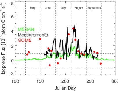
Figure I-4 shows the seasonal time series of isoprene flux measurements compared with models (MEGAN) and satellite (GOME), featuring an increase from leaf-out to early August followed by a sharp decline, with large day-to-day variability superimposed. MEGAN (in green) shows generally under-estimation when compared with direct measurements (in black) and also with measurements retrieved by remote sensing (Palmer et al., 2006).
Figure I-4 Isoprene fluxes at the forest site (PROPHET), Michigan during the 2001 growing season. Green and black lines denote MEGAN and measured isoprene fluxes, respectively. Red circles denote isoprene fluxes retrieved from a 6-year (1996– 2001) formaldehyde (HCHO) column data set from the Global Ozone Monitoring Experiment (GOME) satellite instrument. Horizontal dashed lines denote uncertainty in the retrieved HCHO vertical columns (Palmer et al., 2006).
In soils, microorganisms are the major players in the production of VOC. This production is linked to several processes grouped into two major pathways (Figure I-5):