LM-PAFOG : a new three-dimentional fog forecast model with parametrised microphysics

HAL Id: tel-00730498

https://tel.archives-ouvertes.fr/tel-00730498

Submitted on 10 Sep 2012

HAL is a multi-disciplinary open access

archive for the deposit and dissemination of sci-entific research documents, whether they are pub-lished or not. The documents may come from teaching and research institutions in France or abroad, or from public or private research centers.

L’archive ouverte pluridisciplinaire HAL, est destinée au dépôt et à la diffusion de documents scientifiques de niveau recherche, publiés ou non, émanant des établissements d’enseignement et de recherche français ou étrangers, des laboratoires publics ou privés.

Matthieu Masbou

To cite this version:

Matthieu Masbou. LM-PAFOG : a new three-dimentional fog forecast model with parametrised micro-physics. Océan, Atmosphère. Université Blaise Pascal - Clermont-Ferrand II, 2008. Français. �NNT : 2008CLF21846�. �tel-00730498�

U.F.R. Sciences et Technologies

ECOLE DOCTORALE DES SCIENCES FONDAMENTALES

N

571

THESE

pr´esent´ee pour obtenir le grade de

DOCTEUR D’UNIVERSITE

Sp´ecialit´e: Physique de l’atmosph`ere

Par Matthieu MASBOU

D.E.A. Climat et Physico-Chimie de l’Atmosph`ere

LMPAFOG

-a new three-dimension-al fog forec-ast model

with parametrised microphysics

Soutenue publiquement le 22 Juillet 2008, devant la commission d’examen:

Rapporteur: Mme Evelyne RICHARD

Rapporteur: M. Thomas TRAUTMANN

Pr´esident: M. Klaas S. de BOER

Examinateur: M. Bernd DIEKKR ¨UGER

Directeur de th`ese: Mme Andr´ea FLOSSMANN

Institute of the University Bonn and the Laboratoire de M´et´eorologie Physique of the University Blaise Pascal. Four years have passed since I started this study and I am glad that it is now over. My odyssey in this foggy environment did not always simplify my task to keep a clear visibility. However it was an extremely enriching experience both from a professional and personal point of view. Looking back at these four years I see a satisfying phase in my life in which I have found many valuable contacts, colleagues and friends. I wish to thank many people which contributed to the realisation of this work. Firstly, I wish to thank my supervisors for their inspiration, confidence and patience: Andreas Bott (my supervisor at the University Bonn) for following my scientific interests and ideas and opening many doors to me, not at least the doors to the fog modelling, and Andrea Flossmann (Laboratoire de M´et´eorologie Physique) for her constant encourage-ments and suggestions.

Special thanks go to my colleagues at the meteorological institute of the university Bonn. I thank them for their support ranging from little everyday matters to open-minded discussions in in-depth scientific mystery. I especially thank Isabel Alberts, Malte Diederich, Susanne Bachner and Annika Schomburg for their support, assistance and

con-tributions to the present work. I would like to thank Felix Ament and Volker K¨ull for

many fruitful exchanges and scientific discussions. I wish to thank Insa Thiele for her infinite patience in correcting my frenglish and her optimism. I thank Burkhard Bebel, Thomas Burkhardt and Marc Mertes for their valuable ”technological” support. I am also grateful to Lucia Hallas, Pia Rosen and Monika Stehle for always helping me in the labyrinth of the administration and in the quest of interesting bibliographic references.

I thank Wolfram Wobrock of the Laboratoire de M´et´eorologie Physique for his help and the stimulating discussions. I am also grateful to Fran¸cois Champeau, Delphine Leroy and Pascal Bleuyard for welcoming me with open arms during my time in Clermont-Ferrand. I thank Jean-Louis Barthout and Eliane Passemard for helping me with bureaucratic issues of the ”co-tutelle”.

The COST action 722 provided me with a lively research environment to work in, and in particular it gave me the opportunity to interact with several multidisciplinary research groups, as well as to get in touch with many people, who supported this work in various

ways. I would especially thank Mathias M¨uller (University of Basel) and Jan Cermak

(University of Marburg) for their genuine passion for research on fog modelling and sa-tellite detection and for the successful and excellent collaboration and their hospitality. I am also grateful to Claus Petersen and Niels Woetmann Nielsen (Danish Meteorological Institute), Harald Seidl and Alexander Kann (ZAMG) and Harold Petithomme (M´et´eo France) for the successfull scientific cooperation in the intercomparison campaign. I thank Mich`ele Collomb for having provided me with many interesting bibliographic references. I wish to thank Wilfried Jacobs (DWD) for helping me with the management of the Eu-ropean campaign.

scientific enthusiasm and his expertise on the high resolution modelling. I am also grate-ful to Wolfgang Adam und Gerd Vogel of the Lindenberg observatory for suppling me validation and intercomparison data.

My stay in Bonn over these years has been enriched by the friendship of many people I had the luck to meet, both inside and outside of the institute, and to whom I am deeply grateful for the amusing time we spent together: Ralf and Michael, who took care of my italian diet and my fitness; Susanne and Annika, who showed me how the scientists bounce; Isabel, who took care of my ”rolling Prince” reserve; Marco, who taughts me the german climatology; Timo, who taughts me Italian, Daniel, Pablo and Steffi, who

fought with me in the overtime of the third set, H¨ubschling, who supervised my coffee

consumption; Judith, who showed me what french-german friendship is; Anja, Robin, Kolli, Kerstin, Linda, Rene, Henning, and many others.

I would like to thank Loic, Aur´elia, Zizou, Omar, Bywalf, Bamby and Guigui for their long-standing friendship. You have always been able to cheer me up with your optimism and your advise.

Finally, I thank my parents for having always strongly encouraged me to invest in my study and personal development, my sister, Adeline, and my brother, Julien, for suppor-ting me through good times and bad times. I have a fantastic family !

Matthieu Masbou Bonn, May 2008

1 Introduction 7

1.1 Motivation . . . 7

1.2 What is fog ? . . . 8

1.3 State of numerical fog modelling . . . 9

1.4 Aim and outline . . . 11

2 The ”Lokal Modell” 13 2.1 Overview . . . 13

2.1.1 Model grid . . . 13

2.1.2 Set of model equations . . . 13

2.1.3 Numerics . . . 15

2.1.4 Data assimilation . . . 15

2.1.5 Initialisation and boundary conditions . . . 16

2.1.6 Parametrisations . . . 16

2.2 Interaction soil/atmosphere . . . 17

2.3 The Planetary Boundary Layer parametrisation . . . 19

2.4 Cloud microphysics scheme . . . 20

3 Implementation for three-dimensional fog modeling: LM-PAFOG 23 3.1 Requirements for three-dimensional fog forecasting . . . 23

3.2 The microphysics parametrisation . . . 24

3.2.1 Activation . . . 25

3.2.2 Condensation/evaporation . . . 26

3.2.3 Sedimentation . . . 28

3.3 Microphysics implementation . . . 29

3.4 Spatial discretisation . . . 29

3.5 Boundary conditions for Nc . . . 31

3.6 Visibility parametrisation . . . 32

3.7 Influence of the microphysics . . . 33

4 Evaluation of LM-PAFOG fog forecasts 37 4.1 Approach . . . 37

4.2 Aims and framework . . . 37

4.2.1 Forecast area and available measurements . . . 38

4.2.2 Occurrence of fog events . . . 40

4.2.3 Model configuration . . . 41

4.3 Statistical evaluation approach . . . 41

4.3.1 Method . . . 41

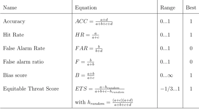
4.3.2 Verification methods for deterministic forecasts . . . 41

4.3.3 Verification results . . . 44

4.3.4 Conclusions . . . 48

4.4 Detailed analysis of LM-PAFOG forecasts of selected fog episodes . . . 49

4.4.1 Method . . . 49

4.4.2 Episode 1, October 6-7th_{, 2005: Radiative fog without cloud cover . 51} 4.4.3 Episode 2, September, 27th _{2005: Radiative fog after a rain event . 65} 4.4.4 Episode 3, December 6-7th_{, 2005: fog influenced by a low stratus . . 70}

4.5 Limits of the soil/atmosphere transfer scheme . . . 76

4.6 Conclusions . . . 78

5 Model intercomparison in the Lindenberg area 79 5.1 Introduction . . . 79

5.2 Intercomparison approach and its limits . . . 80

5.3 Description of the participating models . . . 80

5.3.1 A probabilistic approach to fog forecasts: MOS-ARPEGE (France) 80 5.3.2 The deterministic models . . . 81

5.4 Statistical study . . . 87

5.4.1 A new model: the ensemble forecast . . . 88

5.4.2 Fog intensity and forecast skill . . . 89

5.4.3 Time evolution of fog forecast performances for a visibility threshold of 1000 m . . . 93

5.4.4 Conclusions . . . 96

5.5 Comparison for selected fog episodes . . . 97

5.5.1 Episode 1 - October 6-7th_{, 2005: Radiative fog event without cloud} cover . . . 97

5.5.2 Episode 2 - September 27th_{, 2005: Radiative fog event after a rain} event . . . 108

5.5.3 Episode 3 - December 6-7th, 2005: fog event influenced by very low stratus . . . 117

5.6 Conclusions . . . 127

6 Satellite products for fog and three-dimensional fog forecasts 129 6.1 Description of the satellite products . . . 129

6.2 Comparisons . . . 131

6.2.1 Satellite products quality . . . 133

6.2.2 Results of the verification method . . . 134

6.3 Conclusions . . . 138

7 Conclusions and outlook 139

8 Schlussfolgerung und Ausblick 143

A Analysis of selected fog event-Episode 2: September 27th_{, 2005 151}

B Analysis of selected fog event-Episode 3: December 6-7th_{, 2005 157}

C List of symbols 163

Introduction

1.1

Motivation

Weather can be described in a myriad of dimensions, some of which have a direct effect on humans or on items connected to human well-being. Modern societies have invested in systems to provide information on future weather events. Provision of this information requires expenditure of resources. Societies also wish to understand and assess the real benefits of such forecasts, both as a guide in deciding the most efficient mix of weather products to provide the most useful temporal and spatial dimensions of such forecasts.

Many economical sectors use weather forecasts on a daily or seasonal basis to make decisions. The energy sector uses weather forecasts to estimate fluctuation demands for energy. The household sector uses weather forecasts to make decisions such as what to wear, when and where to go on vacation. The agricultural sector uses precipitation, temperature and frost forecasts to determine when to plant and when to irrigate. The aviation, trucking and shipping sector use weather forecasts to make routing decisions.

Among other weather situations, fog has a significant impact on economical and safety aspects. Numerous traffic management authorities depend strongly on accurate forecasts of fog and visibility (Andre et al., 2004; Pagowski et al., 2004). A study of the French Observatory for Road Safety points out the aggravating role of fog in case of accidents: accidents occurring in foggy conditions double the material damages and furthermore, in case of accidents involving persons, fog constitutes the most aggravating factor with 12 deaths per 100 accidents (Chapelon and Loones, 2001).

Different economic agents request the development of better fog predictions. Studies based on cost/benefit analysis underline the economical value of forecasts on low visibility events (Leigh, 1995; Allan et al., 2001). The National Oceanic and Atmospheric Admi-nistration (NOAA) estimated that improvements of a few hours in forecast for short-term ice formation and fog conditions could save $29 millions per year by rerouting trucks in the transport industry in the United States (NOAA, 2002).

Otherwise, fog does not only appear as an economical issue. In regions with scarce water ressources the development of fog collectors could use fog as a sustainable water source (Schemenauer and Cereceda, 1994).

In terms of traffic safety and economy, human well-being depends on reliable forecasts

of fog occurrence. Temporal evolution, spatial extension and physical properties of fog are the requested information to supply of a forecast. Such a forecast should respect: high spatial resolution, high temporal resolution and fine parametrisation. However, fog forecast quality is still limited because most of todays forecast systems do not meet all these standards.

Necessary improvements have been widely identified. Cooperation and initiatives in the action 722 of the European Science Foundation (ESF) CO-operation in the field of Scientific and Technical Research (COST) programme ensured numerous developments concerning short range forecasting of fog, visibility and low clouds (Jacobs et al., 2005).

A reliable and accurate fog forecast model constitutes an essential support when solving many scientific and socio-economic problems.

1.2

What is fog ?

The presence of fog is defined by a visibility reduction below one kilometer. This mostly happens by suspension of very small, usually microscopic water droplets in the air, redu-cing the horizontal visibility at the Earth’s surface (WMO, 1992). The fog water droplets are considered as having a diameter between 5 and 50 µm (Pruppacher and Klett, 1997),

and settle at velocities of no more than 5 cm s−₁

(WMO, 1996). Generally, most fog

events have a Liquid Water Content (LWC) ranging between 0.01 and 0.3 gm−₃

. More generally, fog formation is considered when water vapour condensates or sublimates on aerosol particles at low altitude.

Fog can be classified into six types depending on its dominating formation process. The processes responsible for the fog formation can be radiative cooling of the ground and the adjacent air masses (radiation fog), cooling of the air parcel below the dew point temperature induced by the advection of air masses over cold surfaces (advection fog), a forced adiabatic cooling of air mass due to topographical obstacles (upslope fog), and atmospheric mixing processes (sea fog, frontal fog and turbulence fog).

Several observation studies of fog have already been done reaching back about 100 years (e.g. K¨oppen, 1916, 1917; Taylor , 1917; Georgii, 1920; Willett, 1928; Roach et al., 1976; Fitzjarrald and Lala, 1989; Leipper , 1994; Kloesel , 1992). These studies emphasised the importance of a multitude of meteorological parameters affecting fog formation and development, including the primary role of radiation, microphysics, turbulence and mois-ture transport over heterogeneous terrain. Formation and dissipation of fog is controlled by continuous interactions between thermodynamic and dynamical factors (Duynkerke, 1991; Roach, 1994, 1995). Furthermore, fog development is affected by the interaction between the land or sea surface and the lower layers of the atmosphere. Local parameters such as topography, vegetation, soil characteristics and very shallow flows near the surface induce small changes that influence fog generation. The large dependence of fog formation on these surface parameters can induce very local formation of fog patches.

1.3

State of numerical fog modelling

The need of a reliable fog forecast and the particularity of fog has led to the development of different forecasting and nowcasting methods based on observations, numerical forecast models and statistic approaches.

Numerical modelling of fog already has a long tradition. The various existing fog mo-dels differ in their complexity describing the relevant thermodynamic and microphysical processes occurring during a fog event. The physical parametrisations of these models fo-cus on partial aspects inducing the formation of fog. Fisher and Caplan (1963) developed one of the first fog models simulating fog evolution. However, they neglected the radiative cooling of the atmosphere. Musson-Genon (1987) and Turton and Brown (1987) concen-trated their efforts on a new formulation of the turbulent transport in the calm nocturnal boundary layer. In others approaches, fog microphysics is considered by parametrisation techniques thus only bulk fog water content can be obtained (Zdunkowski and Nielsen, 1969; Zdunkowski and Barr , 1972; Lala et al., 1975; Brown and Roach, 1976; Bergot and

Guedalia, 1994; Texeira, 1999; Koracin et al., 2001). The bulk microphysics approach is a

severe limitation to accurately describe the gravitational settling of fog droplets. Explicit detailed microphysics considering the time evolution of the spectral size distribution of fog droplets was introduced by Brown (1980) and further refined in a new approach by Bott et al. (1990). Comprehensive description of the interaction between fog and vegetation were developed (Siebert et al., 1992a,b; von Glasow and Bott, 1999). Most of these models have been developed to improve the understanding of local processes in the fog formation. The high grid resolution and the complex parametrisation need significant computation-time efforts. These models favour the modelling of thermodynamics and microphysics at the expense of dynamical factors causing almost all fog models to be one-dimensional. The limitation to a column allows to compute complex parametrisation induced in the fog formation processes very quickly. The interaction soil-atmosphere as well as the descrip-tion of the boundary layer is then well considered. However, a one-dimensional forecast approach assumes horizontal homogeneity of all thermodynamic variables and demon-strates large difficulties to consider dynamical influences induced by their surrounding environment.

Guedalia and Bergot (1994) added in their one-dimensional fog model a forcing

ad-vection term to better reflect its importance in the timing of the fog evolution. Recently, the coupling of a one-dimensional fog model with a three-dimensional mesoscale model illustrates the actual solution to combine the single-column with the surrounding hetero-geneity (Duynkerke, 1999; Texeira and Miranda, 2001; Clark and Hopwood , 2001; Olsson et al., 2007). The atmospheric conditions corresponding to the formation of radiative fog (stable boundary layer, weak advection forcing) can be successfully forecasted in an one-dimensional approach. Nevertheless, single column models are not adapted to treat complex three-dimensional flows. Advection of humid air parcels, cold pools in complex orography and the increase or decrease of the overlying cloud cover are essential factors which cannot be considered in such single-column approaches. Advection fog or orographic fog forecasts cannot be considered by such an approach.

Currently, only mesoscale models consider three-dimensional flows. Ballard et al. (1991) and Golding (1993) used a three-dimensional mesoscale model with parametrised

cloud microphysics to forecast fog. However, fog forecasts using mesoscale models are only possible in a limited way. Such a model can give only coarse information about the formation and dissipation of fog on the scale of a few tens of kilometers. The coarse ver-tical grid (lowest atmospheric layer typically more than 60 m thick) cannot consider the processes involved in fog formation with the necessary accuracy. The details in various parametrisations are significantly limited by the computing time in the three-dimensional forecast approach. Since mesoscale models are designed for the simulation of processes covering large areas, they do not fulfil all the requirements of fog forecasts in a suffi-cient way. Local characteristics as well as detailed thermodynamics and microphysics are overlooked in favour of three-dimensional dynamics consideration.

Certain approaches improve the coarse three-dimensional forecast by implementing additional downscaling which considers the local factor in the fog formation. A few models such as the Unified Model (Cullen, 1993) and the HIRLAM (Petersen and Nielsen, 2000), deliver a direct information on fog presence. The coupling of surface measurements with the mesoscale output can allow effective parametrisation of visibility. However, due to inadequate mesoscale grid resolution, their fog forecasts can only consider cases of widespread fog. In Austria, Seidl and Kann (2002) have developed a post-processing scheme based on the experience of forecasters. They improve the model forecast for the low visibility situation in spite of the large vertical grid. These post-processing approaches increase the reliability of the fog forecast, but the final forecast accuracy is still severely limited by the original horizontal grid resolution. Post-processing is activated only if the coarse mesoscale forecast adequately detects the favourable weather situation.

Local measurements associated with statistic schemes commonly provide an interpre-tation guide for fog forecasts. Statistical methods are based on neural networks (Pasini et al., 2001; Costa et al., 2006; Bremnes and Michaelides, 2007), decision trees

(Wan-tuch, 2001) and regression (Vislocky and Fritsch, 1995; Hilliker and Fritsch, 1999). The

statistical systems require information on the atmospheric profile, which is almost always extracted from a three-dimensional operational forecast model. The forecast variable de-pends on just this profile or both the profile and the latest surface observations. Apart from the input data from each forecast, historical data play a major role when establishing a statistical relationship. It is essential that the historical data and forecast properties of the operational model maintain a constant quality once the statistical relationship is defined. Due to the continuous improvement of the forecast models as well as the diffe-rent measurement devices, this requirement remains difficult to fulfil. Statistic models will work well only if the type of event is well represented in the training data. Most systems appear to have used about three years of historical data. Dense fog events which form rarely in most locations are not sampled adequately in the learning phase which is too brief. The Austrian weather service has developed a Model Output Statistics (MOS) system based on ten years of historical data (Golding, 2002). Both statistical regression and neural networks need such a long historical data set. Moreover, multi-step processes, such as the Perfect-prog method (Klein et al., 1959) as well as the expert system, score table or decision tree approaches always demand a large historical data base, since each step in the process must be calibrated. Most statistical models are site-specific, implying that models developed for one location do not necessarily apply to another. A radical reconstruction of the model may be needed (Mouskos, 2007).

In spite of local fog forecasts, such restrictions inherent to statistical methods consti-tute a significant flexibility deficit in case of further model developments. Moreover, this cascade of statistical treatments disconnects the resulting forecasts from physical fog char-acteristics.

Physically modelling fog forecasts is a complex exercise. No actual fog forecast model is able to consider simultaneously all the requested factors for complete physical model-ling. Interactions between thermodynamic, microphysical and dynamic processes have to be considered simultaneously. The proximity with the ground necessitates the conside-ration of high resolution local factors. Furthermore, the computing power limitation has usually led to neglect parts of the physical or dynamical processes. It appears that the numerical modelling quality and a reliable fog prediction depend on which fog type has to be forecasted. The complexity of various fog formation processes and the consequent inadequacy of simple forecast solutions motivate the engagement into the task of creating a fully physical fog forecast system.

1.4

Aim and outline

In this thesis, a new fog forecast model is developed to combine in one numerical ap-proach all the physical processes to supply a complete fog forecast solution reproducing the miscellaneous fog properties. A new microphysical parametrisation, based on the one-dimensional fog forecast model, PAFOG (Bott and Trautmann, 2002), was implemented in the ”Lokal Modell” (LM) (Steppeler et al., 2003), a nonhydrostatic operational mesoscale model of the German Meteorological Service. The flexibility of the LM’s three-dimensional dynamical core allows numerical simulations in a high resolution grid. The detailed mi-crophysics, PAFOG, offers an accurate computation of condensation/evaporation as well as sedimentation of cloud water which is a decisive factor in the evolution of a fog episode. The three-dimensional framework can resolve the accumulation of cold air and definitely solves the problem of advection forcing. LM-PAFOG is thus a new fog forecast method for simulating different kinds of fog, such as radiation fog, advection fog as well as orographic fog.

After an overview of the basic LM model frame, the low atmosphere parametrisation and cloud microphysics are detailed in Chapter 2. The requirements for the transformation of the LM into a fog forecast model and further implementations concerning the high grid resolution, the new PAFOG microphysics and visibility parametrisation are presented in detail in Chapter 3. A first assessment of the fog forecast model is made and the influence of the new microphysics scheme on fog formation is examined. In Chapter 4, the new forecast model performance is throughly analysed with validation studies and case studies.

A large part of the validation work was done in the framework of the COST 722 project. COST Action 722 is a consortium of scientists from fifteen countries. This cooperation gathers numerous fog forecast models among those: a MOS, a mesoscale model with physical parametrisation of visibility, a three-dimensional operational weather prediction model with post-processing methods and a three-dimensional model with high resolution and detailed microphysics. In Chapter 5, our new fog forecast model is directly confronted

with the performance of the other fog forecast methods in a common statistical evaluation and case studies on the area of Lindenberg (Germany). The potential and the limitations of different models are investigated.

The three-dimensional modelling approach used in our fog forecast model illustrates the limits of the actual measurements necessary for the model assessment. A new verifi-cation approach for the spatial extension of fog using satellite products for fog has been developed and tested on our new three-dimensional fog forecast model, LM-PAFOG. The results are presented in Chapter 6.

The ”Lokal Modell”

Since December 1999, the Lokal Modell (LM) (Steppeler et al., 2003), is a part of the current numerical weather forecast system used by the German Meteorological Service (Deutscher Wetterdienst, DWD). In the last years, the LM has been continuously im-proved and was subjected to many modifications. Today, an international LM user group of six national meteorological services (Germany, Switzerland, Greece, Poland, Italy and Romania) coordinates the futher developments of the LM in the COnsor-tium for Small Scale MOdelling (COSMO). This chapter focuses on the LM version 3.19 used in this work. Further information about the next development can be found at http://www.cosmo-model.org.

2.1

Overview

2.1.1

Model grid

The LM is a nonhydrostatic limited-area numerical weather prediction model, designed to cover all horizontal resolutions from 50km to 50m. In its operational form, the LM uses a horizontal resolution of 7km. Since September 2005, its forecast area has been extended in order to cover all of Europe, yielding the Lokal Modell Europa (LME). The new ver-tical resolution is composed of 40 layers, the height of the lowest layer is 20 meters. The LM grid structure has been adapted to spherical coordinates so that the model domain is almost uniform and avoids regions with strong convergence of the meridians. The poles of the LM domain are defined so that the equator is located within the center of the model domain. Concerning the vertical grid structure, the LM uses generalised terrain-following coordinates with the highest vertical resolution close to the surface.

The discretisation of the prognostic variables is stored on an Arakawa-C-grid (Arakawa, 1966): thermodynamic quantities (pressure, specific humidity and temperature) are de-fined at the centre of a grid box whereas the dynamic variables (wind field, diffusion coefficients and turbulent kinetic energy) are located at the boundaries of the grid boxes.

2.1.2

Set of model equations

The LM is based on non-hydrostatic, fully compressible hydro-thermodynamical equations in a moist atmosphere without any scale approximation. The atmosphere is described

as an ideal mixture of dry air, water vapour, liquid water and water in solid state. The liquid and solid forms of water may be further subdivided into nonprecipitating categories of water such as cloud water and cloud ice with negligible sedimentation fluxes, and precipitating categories of water such as rain, snow and graupel with large sedimentation fluxes. The evolution of the nonhydrostatic compressible mean flow is based on the model equations detailed hereafter (Doms and Sch¨attler , 2002). A complete description of the different variables is summarised in Appendix C.

ρdv dt = −∇p + ρg − 2Ω × (ρv) − ∇ · (T) (2.1) dp dt = − cpd cvdp∇ · v + ( cpd cvd − 1)Qh (2.2) ρcpddT dt = dp dt + Qh (2.3) ρdqv dt = −∇ · F v − (Il+ If) (2.4) ρdql,f dt = −∇ · (P l,f _{+ F}l,f_{) + I}l,f _(2.5) ρ = p{Rd(1 + (Rv Rd − 1)qv− ql− qf)T } −₁ (2.6) (2.7)

Qh represents the rate of diabatic heating/cooling and is given by

Qh = LvIl+ LsIf _{− ∇ · (H + R)} (2.8)

In these chosen approach, the continuity equation, usually one of the primitive equations, has been replaced by a prognostic equation for the pressure. To allow a useful application of the linearisation assumptions related to the anelastic approximation, an hydrostatic reference state of the atmosphere is defined following the method of Dudhia (1993). By introducing the base state, any grid-scale thermodynamic variable ψ can be formally written as:

ψ(λ, ϕ, z, t) = ψ0(z) + ψ

′

(λ, ϕ, z, t) (2.9)

The prognostic equation for the pressure is thus the same for the pressure perturbations. The set of equations supplies a complete description of the state variable, where v is the

barycentric velocity, T is the temperature, p is the pressure, ρ is the air density, qv, ql and

qf are the mass fraction of water vapour, liquid water and ice. To determine the variables

of state, many terms concerning the subgrid-scale processes have to be known. These are the Reynolds stress tensor T, the turbulent flux of sensible heat H, the turbulent fluxes of

water vapour Fv_{, liquid water F}l _{and ice F}f_{. The knowledges of the precipitation fluxes}

of water and ice Pl _{and P}f_{, the rates of phase changes of water and ice I}l _{and I}f_{, and the}

flux of solar and thermal electromagnetic radiation R are also required. The determina-tion of these terms as funcdetermina-tions of the model variables is done in adequate parametrisadetermina-tion schemes, as detailed in the following section.

2.1.3

Numerics

Based on this unfiltered equation system, the LM considers the processes of each scale, even the fast-moving sound waves. These acoustic fast waves, which are meteorologically unimportant, severely limit the time step of explicit time integration schemes. Very small time steps are necessary to fulfil numerical stability. In order to improve the numerical efficiency, the LM integration scheme uses the mode-splitting time integration method proposed by Klemp and Wilhelmson (1978). This technique separates the prognostic equations in terms of fast and slow modes. All terms which describe sound or gravity wave processes are integrated on a small time step. The other terms, which consider meteorological evolutions like advection and physical processes are calculated for longer time steps and stay constant during the integration of the small time step. By default, the numerical time integration scheme follows a Leapfrog scheme of second order accuracy. Alternatively, two other time integration schemes are implemented: a two time-level se-cond order Runge-Kutta split explicit scheme (Wicker and Skamarock , 1998) and a three time-level semi-implicit scheme (Thomas et al., 2000). The LM numerical scheme also has to find a compromise for the ratio of horizontal grid spacing (∼ 10 km) to vertical grid size (∼ 100 m) and the numerical stability of the integration scheme needing a very small time step to consider the vertical sound propagating waves. In order to overcome this problem, horizontal advection of fast and slow modes are explicitly solved, whereas for stability reasons, vertical advection and vertical turbulent diffusion are treated implicitly by the Crank-Nicolson scheme (Crank and Nicolson, 1947).

2.1.4

Data assimilation

The data assimilation approach is based on a nudging method developed by Schraff (1997) and Schraff and Hess (2003). This technique corresponds to adjust the prognostic varia-bles supplied by the model with the available observations.

∂

∂tψ(x, t) = Fψ(x, t) + Gψ·

X

kobs

(Wk_{· (ψk}obs_{− ψ(x}k, t))) (2.10)

Fψ denotes the physical parametrisations and model dynamics, ψobs

k is the kth observation

influencing gridpoint x at time t, xk is the position of the observation, Gψ is a constant

called nudging coefficient and Wk an observation-dependent weight, varying between 0

and 1. The timescale covering the relaxation process is controlled by the coefficient Gψ.

The deviation between the observed value and the model value reduces in about half an hour to 1/e. In practical applications, the nudging term should remain smaller than the largest term of the dynamics or physics for not disturbing the equilibrium of the model. The variables being nudged are horizontal wind, temperature, and humidity at all levels, and pressure at the lowest model level. The analysis increments are adjusted hydrostatically to avoid uncontrolled sources in the vertical wind component. Concerning the soil water content, direct measurements are rarely available. A soil moisture analysis scheme has also been developed so that the 2-m temperature would correspond to the observed temperatures. This correction is done by minimising a cost function (Hess, 2001).

2.1.5

Initialisation and boundary conditions

The definition of the LM domain as a limited area requires lateral boundaries and their time evolution must be specified by an external data set. After the nudging operation,

ini-tial and hourly external boundary conditions are supplied by a coarse-grid model (GME1_,

ECMWF2_{, LM). In its operational form, the LM lateral boundary data are supplied by}

the operational hydrostatic model GME via a one-way interactive nesting using the re-laxation scheme of Davies (1976). In a lateral boundary zone (about eight grid points wide), the prognostic values are gradually nudged in the model domain. This reduces the generation of numerical noise, which can propagate from the lateral boundaries inward to the center of the model domain. The top boundary condition is defined by a rigid lid and a Rayleigh damping layer in order to avoid a backscatter of waves at the upper boundary (Doms and Sch¨attler , 2002).

2.1.6

Parametrisations

The subgrid scale processes such as turbulence, convection and radiation play a determi-nant role on the resolved scale. However, not all relevant physical atmospheric processes can be resolved by the model grid resolution. Physical parametrisations have to be in-cluded in order to consider the influence of sub-grid scale processes. The LM is based on a complete parametrisation set, considering all the relevant sub-grid scale processes.

The radiation scheme is based on a δ-two-stream version of the radiative transfer equation incorporating the effects of scattering, absorption and emission by cloud droplets, aerosols and gases in each part of the spectrum (Ritter and Geleyn, 1992). Sub-grid scale clouds are considered by an empirical function, depending on relative humidity, height and convective activity.

The cloud microphysics module uses a bulk microphysics parametrisation including water vapour, cloud water, ice, rain and snow. The precipitation can either be diagnosed or included in a three-dimensional prognostic precipitation transport scheme. Moist con-vection is parametrised by the mass flux concon-vection scheme of Tiedtke (1989) with a closure based on moisture convergence.

Subgrid scale turbulence is parametrised with a diagnostic second order K-closure for the vertical fluxes. Optionally, a prognostic Turbulent Kinetic Energy (TKE) closure at level-2.5 closure developed by Mellor and Yamada (1982) can be used. The interaction between surface and atmosphere are parametrised with a stability-dependent drag-law formula of momentum, heat and moisture according to the Louis scheme (Louis, 1979).

This thesis focuses on the development of a fog forecast model based on the LM. The thermodynamic and dynamical processes taking place in the lowest atmosphere have a crucial impact on fog formation. Consequently, the actual parametrisation such as turbu-lence, heat and moisture transport at the surface and microphysics scheme are presented in more detail in the next two sections.

1

The expression GME is a combination of its predecessors: GM, Global Model and EM. Europa Model

2

2.2

Interaction soil/atmosphere

The boundary conditions at the surface play a decisive role because they correspond to source and sink term for the atmospheric heat and moisture. In the approach chosen in the LM, the coupling between atmosphere and the underlying surface is based on a stability and roughness-length dependent surface flux formulation which is based on a modified Businger relation (Businger et al., 1971). These surface fluxes constitute the lower boundary conditions for the atmospheric part of the model. In this drag-law formulation, the heat and moisture fluxes are defined in a linear relation.

The surface flux of sensible heat Ft _{is defined accordingly:}

Ft_{= −ρKh|vh|(Tatm− Tsf c}) (2.11)

where ρ is the air density, Kh _{is the heat transfer coefficient, |v}h| is the absolute wind

speed in the lowest atmospheric layer, Tatm is the temperature of the lowest atmospheric

layer and Tsf c is the temperature at the ground.

For the moisture flux, Fv

sf c, at the surface, the parametrised relation is defined as:

Fv_{sf c} = ρK_h|vh|(qv_{atm− qsf c}) (2.12)

where qv

atm is the specific humidity in the lowest atmospheric layer and qsf c is a virtual

specific humidity at the surface. The transfer coefficients are determined diagnostically as a function of the bulk Richardson number (see Section 2.3)

In this approach, the moisture flux is deduced by the balance involved by the evapo-transpiration parametrisation while the temperature at the ground is obtained from a balance equation for the heat fluxes at the surface. The soil model TERRA provides the necessary thermal and hydrological processes in the soil, as well as the vegetation influence to complete the balance equation. Interception storage (e.g. lake, sea), snow and nine different soil types are considered. Depending on the season, the consideration of the soil surface diversity is completed with further parameters: roughness length, plant characteristics (plant cover, leaf area index, root depth). Each soil type is defined by different physical parameters, like pore volume and heat conductivity (Doms et al., 2005). The interface soil/atmosphere is thus formulated by two coupled equations for the heat and moisture budget at the ground:

0 = Ft(Tsf c) + Lv(Tsf c)F_{sf c}v (ηg, Tsf c) + Qrad,net+ Gp+ Gs+ Fh(ηg, Tsf c) (2.13)

(1 − fi− fs)(1 − fveg)Eb(Tsf c) + fvegEtrans(Tsf c, ηg) + fiEi+ fsEs= −Fv(qatm) (2.14)

In the heat budget equation (eq. 2.13), Qrad,net is the total radiation budget at the

surface. Ft _{and F}v

sf c are the turbulent atmospheric fluxes of heat and water vapour at

the ground (eq. 2.11 and 2.12 ). Gp and Gs account for the effects of freezing rain and

melting snowfall, respectively, while Fh is the heat flux within the soil.

At the surface, rain and snow are partially captured by the interception store and the snow store. Both surface storages are continuously in interaction with the atmosphere

through evaporation and sublimation as well as dew and rime processes. The soil moisture storage is reduced by evaporation of bare soil and plant transpiration. The global evapo-transpiration at the surface is detailed by the contributions of bare soil evaporation Eb,

plant transpiration Etrans, evaporation of the interception store Ei and snow sublimation

Es depending on the fraction of surface covered by snow fs, water fi and plants fveg .

Finally, Tsf c and ηg are respectively the temperature and the volumetric moisture

content at the ground. These two parameters must still be determined in order to satisfy the heat and moisture budget (eq. 2.13 and 2.14) at the surface.

The heat soil flux Fh at the ground, necessary to complete the heat budget at the

surface is assumed to be:

Fh(ηg, Tsf c) = λ ∂T ∂z ¯ ¯ ¯ ¯ sf c (2.15) where λ is the heat conductivity in the soil.

The vertical soil water flux Fη is described following the one-dimensional Darcy

equa-tion (see standard textbook, e.g. Dingman, 2002)

Fη _{= −ρ}w[−D(η)

∂η

∂z + K(η)] (2.16)

where K(η) is the hydraulic conductivity and D(η) is the hydraulic diffusivity. Both pa-rameters depend on soil characteristics and on soil moisture according to Rijtema (1969):

D(η) = D0exp · D1 ηP V − η ηP V − ηADP ¸ (2.17) K(η) = K0exp · K1 ηP V − η ηP V − ηADP ¸ (2.18)

The four constants K0, K1,D0, D1, as well as the pore volume ηP V and the soil moisture

at air dryness point ηADP depend on the soil type (Doms et al., 2005).

To solve the heat and moisture budget at the surface, the vertical profile of temperature

Tso and moisture η in the soil have to be determined. The soil model TERRA can either

solve the heat conduction equation and soil water transport in its two soil layers version through the extended force restore method (Jacobsen and Heise, 1982) or in its new operational multilayer version (Schrodin and Heise, 2001) by a direct numerical solution of the following equations.

∂Tso ∂t = 1 ρc ∂ ∂z µ λ∂Tso ∂z ¶ (2.19) ∂η ∂t = ∂ ∂z µ D(η)∂η ∂z + K(η) ¶ (2.20) The volumetric heat capacity ρc is determined by taking the values for dry soil, water and ice into account. The parametrisation of the heat conductivity λ considers only the liquid water content of the soil. The soil moisture and soil temperature are thus prognostically

determined. At each time step, Tg and ηg can be determined and the heat and moisture

2.3

The Planetary Boundary Layer parametrisation

to derive the bulk transfer coefficients for heat Kh and for momentum Km at the surface

(Monin and Obukhov , 1954). But the Monin-Obukhov length, necessary to determine the flux-profile depends itself on the fluxes. To avoid a costly computation of an iteration method, Louis (1979) proposed an analytic procedure using the bulk Richardson number, RiB, as a stability parameter.

RiB = g

θsf c

(θatm_{− θ}sf c)(h − z0) |vh|2

(2.21)

where θsf c and θatm are the potential temperature respectively at the surface and in the

lowest model atmospheric layer, z0 is the roughness length and h corresponds to the

Prandtl layer thickness. The lowest model layer (about 60 m thick) is assumed to be located within the Prandtl layer

Using the bulk Richardson number, the stability evolution at the surface can be simply determined by known temperature and wind profiles. The transfer coefficients are thus defined as follows: Km = µ κ ln(h/z0) ¶2 fm(RiB, h/z0) (2.22) Kh = κ 2 ln(h/z0) ln(h/zh)fh(RiB, h/z0, h/zh) (2.23)

where κ is the von-Karman constant, zh is the roughness length for heat exchange and fm

and fh are stability functions in the constant flux layer. fm and fh are chosen to include

the limiting cases of free convection and of laminar flow in a highly stable surface layer. The influence of the surface through exchange of heat and moisture is not limited to the lowermost atmospheric layer of the model. In the lowest part of the atmosphere, the moisture and heat are transported mostly by turbulent processes. In the LM, where the horizontal grid scale is large compared to the vertical grid resolution, the vertical turbulent transport is considered to be dominating so that the horizontal turbulences are neglected. Turbulence can be parametrised by the K profile-theory which relates the subgrid scale flux to the vertical atmospheric gradient. For the momentum transport, the vertical turbulent flux is given by:

w′_u′ = −Kmv ∂u ∂z, w ′_v′ = −Kmv ∂v ∂z (2.24)

The turbulent heat and moisture transports are expressed similarly: w′_θ′ = −Khv ∂θ ∂z, w ′_q′ v = −Khv ∂qv ∂z (2.25)

where u and v are the horizontal wind components, θ is the potential temperature, qv is

the mass fraction of water vapour, and Kv

m and Khv are the turbulent diffusion coefficients

for momentum and heat.

To calculate the turbulent fluxes, the Louis scheme (Louis, 1979) is used again. As stability parameter, the Richardson number Ri is defined by a ratio involving the squared

Brunt-V¨ais¨al¨a frequency, N2_{, corresponding to the buoyancy influence and the influence}

of vertical wind shear, M2_:

Ri = N 2 M2 = g θv ∂θv ∂z ¡_∂u ∂z ¢2 +¡_∂v ∂z ¢2 (2.26)

The turbulent diffusion coefficients Kv

m and Khv are determined as:

Kv

m = l2Sm3/2(Ri)pM2− αnSh(Ri)N2 (2.27)

Kh = αnSh(Ri)K_mv (2.28)

where Sm(Ri) and Sh(Ri) are the stability functions for momentum and heat transport de-pending on the Richardson number. The turbulent length scale is parametrised according to Blackadar (1962):

l = κz

1 + κz/l∞ (2.29)

where z is the altitude. The turbulent length varies at low altitude before reaching its

asymptotic value l∞, set to 500m.

Although the Louis scheme provides an analytical solution to compute the turbulent mixing, this approach has to be completed in case of very stable stratification. The stability functions diverge from the physical solution when the Richardson number exceeds a critical value. For the case Ri > Ric, the diffusion coefficients are corrected as follows:

K_mv = km0l2M2 (2.30)

K_hv = αnkh0l2M2 (2.31)

where the different constants are defined as Ric= 0.38, km0= 0.010, kh0 = 0.007, αn= 1.

2.4

Cloud microphysics scheme

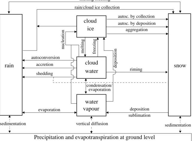
The LM cloud microphysics are computed using a bulk microphysics parametrisation based on the Kessler scheme (Kessler , 1969). In its operational form, the LM runs with a two-category ice scheme, including five categories of water: water vapour, cloud water, ice, rain and snow. Water vapour, cloud water, as well as cloud ice represent the cloud phase and have a negligible fall velocity. Snow is considered as an aggregate of ice crystals having a non-negligible fall velocity. Rain and snow represent the precipitable phase. In order to describe adequately mixed phase clouds the condensation/evaporation processes of cloud water and depositional growth of cloud ice at temperature below the freezing point are considered as two distinct processes of the bulk microphysics scheme. The time

scale of the Bergeron-Findeisen process which defines the initial growth of ice particles confirms this hypothesis. It is generally much smaller than the characteristic dynamic time scale of stratiform clouds (Bergeron, 1935).

In a bulk scheme as used in LM, assumptions are made concerning the shape and the size distribution of the particles and microphysical processes have to be parametrised in terms of specific vapour, water and ice concentration. The depositional growth of cloud ice requires assumptions on shape, size and number density of crystal. Cloud ice is assumed to consist only of small hexagonal plates. The density of cloud ice particles is defined as a function of the ambient temperature based on the Fletcher-formula (Fletcher , 1962) and adapted with aircraft measurements of pristine crystals in stratiform clouds (Hobbs and Rangno, 1985; Meyers et al., 1992). The non-precipitating categories are assumed to be monodisperse whereas the precipitation particles follow an exponential size distribution with respect to particle diameter. For raindrops, it is based on a Marschall-Palmer distribution (Marschall and Marschall-Palmer , 1948), while for snow the Gunn-Marshall distribution (Gunn and Marshall , 1958) is assumed.

evaporation

Precipitation and evapotranspiration at ground level

deposition sublimation riming sedimentation _{sedimentation} deposition melting/freezing rain/cloud ice collection

cloud

ice

cloud

water

water

vapour

rain

snow

Figure 2.1: Cloud microphysic processes in LM: standard two-category ice scheme. The different cloud microphysics processes of the two-categories ice scheme are illus-trated in Figure 2.1. When a sufficient amount of cloud water or cloud ice is produced, the cloud water or ice particles are converted in raindrop or snow. By collision-coalescence processes the formation of raindrop is initiated (autoconversion). The rain or snow mass

fraction can be further increased by collection of others snowflakes, cloud droplets (ac-cretion or aggregation). Depending on the temperature and humidity condition, the precipitation species may convert from rain to snow or vice versa and may also partially or completely evaporate before reaching the earth’s surface.

To complete this microphysics scheme, the condensation/evaporation processes have to be parametrised. The calculation of condensation and evaporation rates, Sc, is based on an instantaneous saturation adjustment technique within clouds. If a grid box be-comes supersaturated with respect to water during a time step, the temperature and

concentration of water vapour, qv and cloud water, qc, are isobarically adjusted to a

sa-turated state, taking latent heating into account. This phase transition is considered to be instantaneous. In this bulk approach, the nucleation process is strongly simplified. It is assumed that there is always a sufficient number of Cloud Condensed Nuclei (CCN) present to initiate the condensed water phase in case of supersaturation. As a closure for the saturation equilibrium, condensation/evaporation is treated as a quasi-reversible

process with only two different thermodynamic states: saturated condition with qc > 0

and subsaturated no-cloud case qc = 0. Clouds always exist in case of water saturation

Implementation for

three-dimensional fog modeling:

LM-PAFOG

3.1

Requirements for three-dimensional fog

forecas-ting

A three-dimensional fog model requires detailed cloud microphysics and should be able to run at spatial high resolutions. Horizontal resolution is an important factor when conside-ring the different air flows and stagnant air pools induced by the topography. Moreover, the generation of a temperature inversion in the boundary layer is a determinant step in a potential formation of fog. The boundary layer also needs a very high vertical resolu-tion. The dynamics core of the LM is a suitable tool for the fog forecast. The ”Lokal Modell” is a fully compressible nonhydrostatic model, designed to cover various horizon-tal resolutions ranging from 50 km down to 50 m (Doms and Sch¨attler , 2002). In the fog formation, the condensation/evaporation processes as well as the cloud droplet se-dimentation are crucial. However, the operational use of the LM induces the presence of highly simplified parametrisation in order to restrain the computation time. In the LM, the condensation/evaporation is based on a bulk saturation adjustment scheme (Sec-tion 2.4). The driving scheme separates condensa(Sec-tion from evapora(Sec-tion with a relative humidity threshold value (usually 100%). In case of coarse resolution, the relative hu-midity threshold is rarely reached: the large volume of the grid box is often filled with partial cloudiness. These clouds have to be correctly forecasted in order to represent the interactions with radiation, and thus with the energy balance. More sophisticated con-densation/evaporation schemes are already available. In the formation of cloud droplets, the supersaturation conditions detailed by K¨ohler (1936), are conducted by the chemical composition and the size of the aerosols. Bigger aerosol particles and higher salt con-centration decrease the critical point of supersaturation. For very small moist aerosol particles the contained salts allow the formation of droplets at relative humidity below 100%. Larger droplets grow when the smaller ones are already evaporated. To model these different processes, the droplet growth equation is solved for several droplet size bins as it was done in some one-dimensional models (Brown, 1980; Flossmann et al.,

1985; Bott et al., 1990) as well as in three-dimensional models (Leporini, 2005). However, the implementation of such microphysics schemes are computationally too expensive to be used for actual weather forecasting. The microphysics of our three-dimensional fog forecast model is an intermediate solution based on the K¨ohler theory so that only a total droplet number concentration has to be considered. The microphysics scheme still has a high degree of sophistication and the computation time is strongly reduced.

3.2

The microphysics parametrisation

The microphysics parametrisation is based on the one-dimensional fog forecast model, PAFOG (Bott and Trautmann, 2002). This parametrisation scheme introduces the cloud

droplet concentration, Nc as prognostic variable. The cloud liquid water content in the

lower part of the model atmosphere is thus controlled by this new variable, Nc, and the

specific cloud water content, qc. The prognostic equations for these variables are given

by: ∂Nc ∂t = v · ∇Nc+ ∂ ∂z µ K_hv∂Nc ∂z ¶ +µ ∂Nc ∂t ¶ P AF OG (3.1) ∂qc ∂t = v · ∇qc+ ∂ ∂z µ K_hv∂qc ∂z ¶ +µ ∂qc ∂t ¶ P AF OG (3.2)

The first two terms on the right hand side describe advection and turbulent mixing pro-cesses, computed by the dynamic core of the LM. The third term gathers the influences of the the PAFOG microphysic processes, i.e. sedimentation of cloud droplets as well as the source and sink caused by the phase changes between the gaseous and liquid phase. Before defining the different processes of the parametrisation, an assumption on the droplet size distribution has to be made. In PAFOG, this is described by a log-normal function. dNc= _√ Nc 2πσcDexp · − 1 2σ2 c ln2µ D D0 ¶¸ dD (3.3)

where D is the droplet diameter, D0is the mean value of D and σcis the standard deviation

of the given droplet size distribution. According to Chaumerliac et al. (1987), this quantity

may be chosen as function of the particular aerosol type (maritime: σc= 0.28, continental:

σc = 0.15). In our microphysics scheme, a constant value of σc = 0.2 is used. Only by

the computation of the mean diameter, the microphysics scheme is able to consider the variation of the cloud droplet concentration. The selected distribution shape corresponds to the generally computed spectral distribution (Bott, 1991) or measurements (Colomb et al., 2007).

In this fixed microphysics framework, the following two prognostic equations are solved with the PAFOG microphysics core. Sedimentation of cloud droplets and the source-sink

terms describe phase changes between the gaseous and liquid phase. µ ∂Nc ∂t ¶ P AF OG = µ ∂Nc ∂t ¶ act + ∆(S)µ ∂Nc ∂t ¶ eva +µ ∂Nc ∂t ¶ sed (3.4) µ ∂qc ∂t ¶ P AF OG = µ ∂qc ∂t ¶ con/eva +µ ∂qc ∂t ¶ sed (3.5) ∆(S) = ½ 1, for S < 0 0, for S > 0 (3.6) S = qv qv sat − 1 (3.7)

where S is the mean supersaturation, qv is the specific humidity and qv

sat is the specific

humidity value at saturation. We note that with the ∆(S) mechanism, the evaporation

modifies Nc only if the air is unsaturated.

With the introduction of Nc as a new prognostic variable, the parametrisation of the

cloud evolution is significantly improved. Contrary to the original mesoscale microphysics scheme, the cloud liquid water content is defined as a concentration of water droplets, giving more information about the microphysic structure of the cloud. The interactions

between Nc and liquid water are quite complex: an increase in liquid water does not

necessarily change the droplet number concentration. Existing droplets may grow without new droplets being formed. The cloud evolution is thus controlled by the evolution of Nc. The cloud formation is initiated by an activation process. The coupling between the ∆(S) mechanism and the one moment droplet size distribution is able to consider first the evaporation of the smallest cloud droplets. Also the sedimentation can increase

or decrease Nc and cloud water, depending on the size of the settling droplets. At the

ground, liquid water is treated like precipitation and droplets disappear due to deposition. The three parts of the PAFOG microphysics, activation, condensation/evaporation and sedimentation, are detailed hereafter.

3.2.1

Activation

The PAFOG microphysics needs an assumption about the number of activated cloud con-densed nuclei when supersaturation is reached. Different authors (Squires, 1958; Twomey, 1959) have developed parametrisation of the nucleation process in order to avoid a difficult supersaturation forecast as well as a fine physical and chemical property description of the studied air parcel. Therefore, for a supersaturation S, the number of activated cloud

droplets, Nact is calculated according to Twomey’s relation (Twomey, 1959):

Nact= NaSk (3.8)

where Nais the Cloud Condensed Nuclei (CCN) concentration, and k are empirical

cons-tants which depend on the environment (maritime: Na = 100 cm−3, k = 0.7, continental:

Na = 3500 cm−₃

, k = 0.9). In the present version, the aerosol concentration values were

set constant in space and in time. For our study in Germany, we chose Na = 10000 cm−₃

The increase in total concentration of cloud droplets during a time step ∆t represents the first term of (3.5), ¡_∂Nc

∂t ¢

act and with Twomey’s relation is written as:

Nc(t + ∆t) = Nc(t) + max(Nact_{− N}c(t), 0) (3.9)

With the maximum operator, Nc only increases in case of a positive tendency in the

supersaturation. Therefore if the supersaturation remains unchanged or decreases no new droplets are activated and the already existing droplets grow.

3.2.2

Condensation/evaporation

The parametrisation for the condensation and evaporation of cloud droplets is based on the works of Nickerson et al. (1986) and Chaumerliac et al. (1987).

After the activation process the time evolution of the cloud is controlled by the time rate of change for the cloud droplet diameter D due to condensation or evaporation (Pruppacher

and Klett, 1997) and is expressed as:

dD

dt = Gf

S

D (3.10)

where S is the supersaturation (see eq. 3.7). The ventilation coefficient is, f = _{−4.33 · 10}5_D2

+5.31 · 103_{D + 0.572 (Pruppacher and Rasmussen, 1979) and G, the following}

thermody-namic function: G = 1 Lvρw KT ³ Lv RwT − 1 ´ + ρwRwT ev sat(T )Dv (3.11) where ev

sat is the saturation vapour pressure over a plane water surface, Rw the specific gas

constant for moist air, Dv the water vapour diffusivity and K the thermal conductivity.

The time evolution of the specific cloud water due to condensation or evaporation processes is then defined as:

µ ∂qc ∂t ¶ con/eva = ρw ρ ∞ Z 0 π 2D 2dD dt dNc(D) dD dD (3.12)

Replacing dD_dt by (3.10) and introducing the log-normal distribution for the cloud droplets

concentration, we find: µ ∂qc ∂t ¶ con/eva = ρw ρ π 2GSNcD0exp µ σ2 c 2 ¶ (3.13)

In case of evaporation, the smallest droplets disappear first and Ncdecreases. From (3.10),

we can deduce the critical droplet diameter, Dc,eva of the biggest droplets still evaporated

in a time step: 0 Z Dc,eva DdD = t+∆t Z t GSdt (3.14)

Considering G and S constant over the time step, we finally have: Dc,eva =

√

Integrating from the smallest droplet to the critical diameter, we obtain: Nc_|eva = Dc,eva Z 0 Nc(D)dD (3.16)

Therefore the loss in droplet number concentration due to evaporation, ¡_∂Nc

∂t ¢

eva can be

integrated on a time step ∆t as

Nc_{(t + ∆t)|}eva = Nc(t) − Nc|eva (3.17)

During the condensation/evaporation processes, the supersaturation S has to be known. Because of the discrepancy between the supersaturation time constant and a reason-able model time step integration, it is not possible to calculate S exactly. However,

Sakakibara (1979) proposes a solution corresponding to the supersaturation mean value

on the integration time step. Moreover, the solution is numerically stable for any time step values and for any cloud droplet concentration values. Finally, the precision of the solution increases with the decrease of the time step. The analytical solution is based on the macroscopic prognostic equation for supersaturation:

dS dt = µ S + 1 p − 0.623(S + 1) RT2 Lv ρacpd ¶ dp dt + µ 1 qv sat +0.623(S + 1)L 2 v RT2_cpd ¶ ∂qv ∂t (3.18) with dp dt = −ρagw (3.19) ∂qv ∂t = − ∂qc ∂t|con/eva (3.20)

where P , T and w are pressure, temperature and vertical velocity respectively; qv

sat is the

specific humidity value at saturation, Lv is the latent heat of vaporisation, g is the

accele-ration of gravity and cpd is the heat capacity for dry air at constant pressure. Introducing

the results of the equation (3.13), the time dependence of the supersaturation S is given by: dS dt = (c1+ c2+ c3)S + c3 (3.21) where c1 _{= −} 1 qv sat ρw ρ π 2GΣc (3.22) c2 = − L2 v RT2_cpd ρw ρ π 2GΣc (3.23) c3 = µ 1 p − Lv RT2_ρcpd ¶ dp dt (3.24) Σc = NcD0expµ σ 2 c 2 ¶ (3.25)

By solving the previous equation, a mean value for the supersaturation, S, over the time step ∆t is then deduced:

S = −c3_c −³S(t) + c3 c ´µ 1 − ec∆t c∆t ¶ (3.26)

where S(t) is the supersaturation at the beginning of the time step ∆t and c = c1+c2+c3.

Knowing the supersaturation, we can quantify the influence of the phase changes on the liquid water content, the specific humidity and the temperature:

∂qc ∂t con/eva = ρw ρ π 2GSΣc (3.27) ∂qv ∂t con/eva = − ρw ρ π 2GSΣc (3.28) ∂T ∂tcon/eva = − Lv cpd ∂qv ∂t |con/eva (3.29) (3.30)

3.2.3

Sedimentation

Fog events are linked with calm synoptic situations, where the vertical wind velocity is very weak. The sedimentation of cloud droplets has to be considered. Thus, the sedimentation tendencies for cloud water and condensation nuclei are defined as:

µ ∂Nc ∂t ¶ sed = ∂Sn,c ∂z − ∂(wNc) ∂z (3.31) µ ∂qc ∂t ¶ sed = ∂Sq,c ∂z − ∂(wqc) ∂z (3.32)

where Sn,cand Sq,c are the sedimentation terms for cloud droplet concentration and liquid

water content (see eq. 3.36 & 3.35).

The formulation of Berry and Pranger (1974) expresses the settling velocity as a function of droplet diameter and the Reynolds number Re

v(D) = ηRe

Dρ (3.33)

where η the coefficient of dynamic viscosity in air, is given as:

η = 1.496286 × 10−₆ T

3/2

T + 120 (3.34)

With the equation (3.33), the sedimentation terms can then be evaluated:

Sn,c= ∞ Z 0 Nc(D)v(D)dD = Ncv(D0) √ 2σcξ exp µ (k2_{− 1)}2 4ξ2 ¶ (3.35)

Sq,c = 1 ρ ∞ Z 0 m(D)Nc(D)v(D)dD = Ncm(D0)v(D0_√ ) 2σcξρ exp µ (k2+ 2)2 4ξ2 ¶ (3.36)

using a2 = 1.01338, a3 _{= −0.0191182 and the following parameters}

ξ = s 1 2σ2 c − 9a 3 (3.37) k2 = 3a2+ 6a3ln(aD30) (3.38) a = 4ρρwg 3η2 (3.39) m(Dc,0) = π 6ρwD 3 0 (3.40)

For the numerical solution of sedimentation, the positive definite advection scheme of Bott (1989) is used. Since the size distribution of the droplets is known, the sedimentation of the droplets can be computed accurately.

3.3

Microphysics implementation

The PAFOG microphysics, detailed in Section 3.2, was implemented in the ”Lokal Mo-dell”. The condensation/evaporation parametrisation, based on a saturation adjustment scheme, was substituted by a detailed microphysics (Figure 3.1). PAFOG microphysics is limited to the lowest part of the atmosphere, currently below 2000 meters (Figure 3.2). In this domain, where fog and low stratus clouds form, the condensation and evaporation processes as well as the sedimentation of cloud droplets are modeled with the PAFOG cloud microphysics. Precipitation, autoconversion, accretion, evaporation of precipitation and processes including the ice phase stay unchanged and are forecasted by the original LM microphysics in the whole atmosphere. Thus, the implementation of the PAFOG microphysics into the LM does not interfere with the already existing cloud and pre-cipitation microphysics scheme of the LM. Liquid water content already is a prognostic variable in the LM. Once formed, this quantity is transported by advection and tur-bulence. The implementation of the PAFOG microphysics introduces the total droplet number concentration, Nc, as a new prognostic variable into the dynamic core of the LM needing horizontal and vertical advection as well as the turbulent transport of Nc. The

three-dimensional link between liquid water and Nc is hereby ensured.

3.4

Spatial discretisation

The fog is strongly dependent on the boundary layer processes such as radiative cooling at the surface and heat and humidity transport at the interface soil/atmosphere. The fog forms close to the surface and grows steadily upwards. The modelling of such processes requires a high vertical resolution. In the actual operational weather forecast models, the lowest layer in the atmosphere is about 20 m thick in the LM. With this coarse grid the fog formation cannot be described.

evaporation

Precipitation and evapotranspiration at ground level

sedimentation _{sedimentation}

melting/freezing rain/cloud ice collection

cloud

ice

cloud

water

rain

snow

water

vapour

Figure 3.1: Cloud microphysic processes in LM-PAFOG: standard LM two-category ice scheme (black part), PAFOG microphysics (red part).

BOUNDARY

Soil Model Nc Fog/Stratus

Nc Nc

Water/Ice Cloud Precipitation

qc

qc

20000 m

2000 m

The determinant evolution for the formation of radiation fog occurs close to the surface. The modelling of the boundary processes can only succeed with a high vertical resolution. In case of a radiative fog event, the surface cooling causes the formation of large tem-perature and humidity gradients in the lowest meter of the atmosphere. From this thin saturated atmospheric layer, the fog grows steadily upward. In our three-dimensional fog forecast model, LM-PAFOG, the high vertical resolution is thus concentrated near the ground: 25 of 40 levels are located in the first 2000 meters and ten layers of 4 meters offer a fine detection of fog formation at the ground. The horizontal resolution should also be rather high to consider the variation of the surface parameters (orography, soil types). A resolution of 2.8 km is presently used and the different air flows and stagnant air pools induced by the topography are thus better modelled.

3.5

Boundary conditions for N

The structure of PAFOG microphysics is based on a new prognostic variable, Nc, the

droplet number concentration. The main goal is to define a clear link between Nc

and the liquid water content qc. The cloud formation processes -activation, condensa-tion/evaporation and sedimentation- allow a more precise modelling of the cloud water concentration. But the PAFOG microphysics core experiences difficulties when forecas-ting cloud cover evolution, if a cloud is transported into the PAFOG domain. In this case, the cloud is only defined by its liquid water content and the PAFOG microphysics is unable to evaporate or sediment this cloud water because there is no correspondence with a droplet concentration. Therefore, liquid water accumulates in an environment that might have a relative humidity far below the saturation and finally may form precipita-tion. This invisible cloud water results from the initialisation of cloud cover at forecast start and from the advection or turbulent diffusion through the lateral boundaries as well as the advection through the top boundary, since PAFOG is restricted to the lowest 2000

meters of the atmosphere. In order to optimise the relation between Nc and liquid water

content, a boundary condition for Nc has to be formulated.

A possible solution is to relate liquid water content at the boundary directly to Nc

assu-ming a lognormal droplet size distribution. We can solve equation (3) of Chaumerliac

et al. (1987) for Nc and thus use it at the boundaries.

qc= Nc ρ ( π 6D 3 0ρw)exp( 9 2σ 2 c) (3.41) Nc= ρqc( 1 π 6D30ρw )exp(−9 2σ 2 c) (3.42)

The credibility of the Ncboundary values depends on the choice of the mean diameter and

the standard deviation defining the lognormal distribution. These parameters values are

based on the work of Miles et al. (2000), who summarises the Ncmeasurement campaigns

in marine and continental environments for low-level stratiform clouds. The Ncboundary

parametrisation detailed hereafter was developed for a continental environment. The Nc

lognormal distribution at the boundary is parametrised with a fixed mean diameter of

10 µm and a variable standard deviation. The value of the standard deviation σcchanges