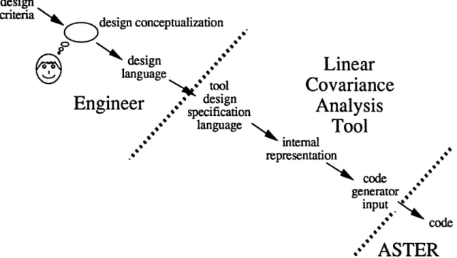
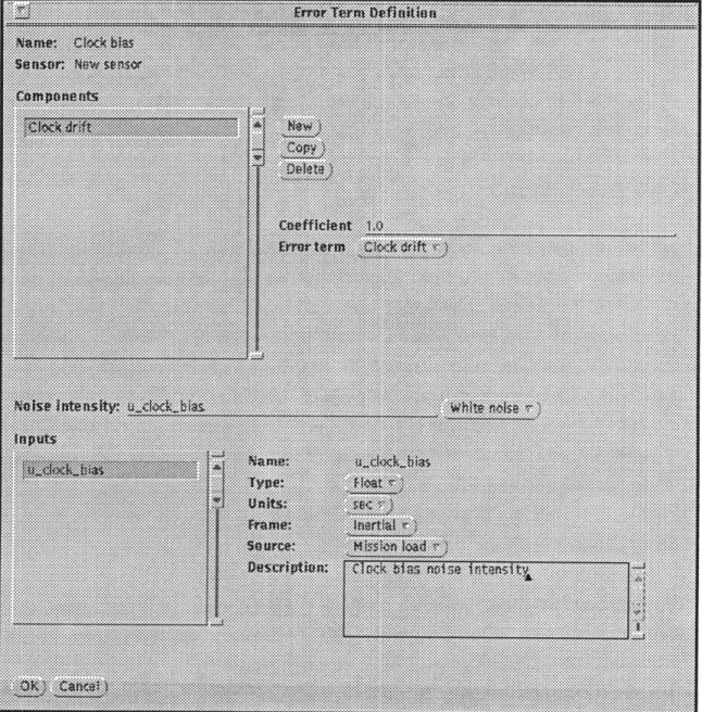
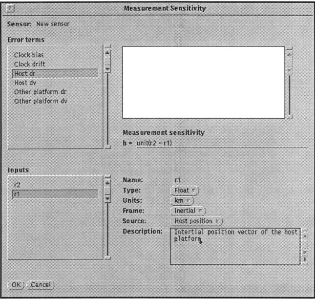
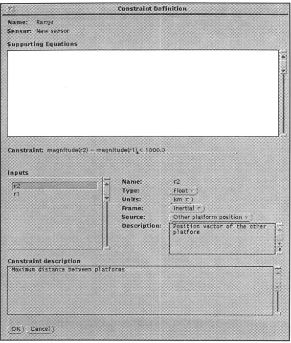
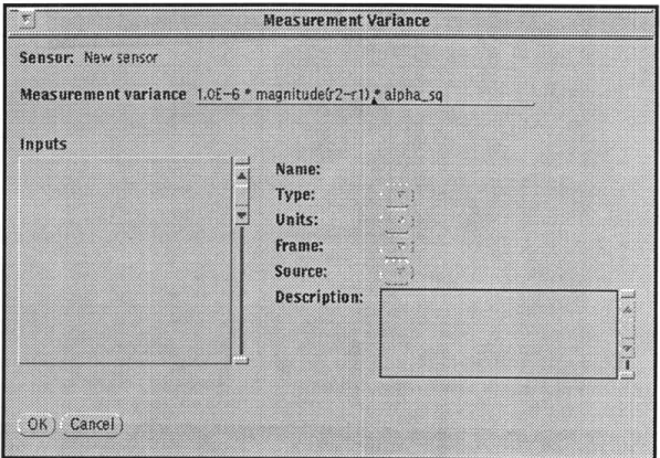
An automated tool for formulating linear covariance analysis problems
Texte intégral
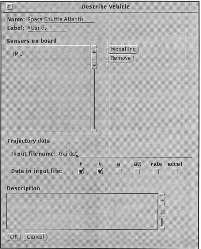
Figure

Documents relatifs
Molecular dynamics, S-model kinetic equation, Evaporation & Condensation coefficient, Liquid-Vapor inter- face, Liquid boundary, Vapor boundary, Kinetic boundary
We then propose conducting an evaluation in different economic situations of a measure devised before the crisis, i.e., tax allowances on overtime hours and their exemption
This sensor is based on variable a reluctance principle. It is a magnetic circuit made up by a fixed part and a mobile one, here one of the rods of the actuator. This sensor
Though numerous studies have dealt with the α− methods, there is still a paucity of publi- cations devoted to the clarification of specific issues in the non-linear regime, such
This special issue entitled “Complex Problem Solving and its Position in the Wider Realm of the Human Intellect” in the Journal of Intelligence comprises several papers, some of
L’archive ouverte pluridisciplinaire HAL, est destinée au dépôt et à la diffusion de documents scientifiques de niveau recherche, publiés ou non, émanant des
A derivation of the energy-position and momentum-time uncertainty expressions for a relativistic particle is a bit “fuzzy” (like space and time in quantum
Abstract: This paper proposes a solution to the problem of velocity and position estimation for a class of oscillating systems whose position, velocity and acceleration are zero
