Architecture design for highly flexible and energy-efficient deep neural network accelerators

(1)

Architecture Design for Highly Flexible and

Energy-Efficient Deep Neural Network Accelerators

by

Yu-Hsin Chen

B.S. in EE, National Taiwan University (2009)

S.M. in EECS, Massachusetts Institute of Technology (2013)

Submitted to the

Department of Electrical Engineering and Computer Science

in partial fulfillment of the requirements for the degree of

Doctor of Philosophy

at the

MASSACHUSETTS INSTITUTE OF TECHNOLOGY

June 2018

c

○ Massachusetts Institute of Technology 2018. All rights reserved.

Author . . . .

Department of Electrical Engineering and Computer Science

May 23, 2018

Certified by . . . .

Vivienne Sze

Associate Professor of Electrical Engineering and Computer Science

Thesis Supervisor

Certified by . . . .

Joel Emer

Professor of Electrical Engineering and Computer Science

Thesis Supervisor

Accepted by . . . .

Leslie A. Kolodziejski

Professor of Electrical Engineering and Computer Science

Chairman, Department Committee on Graduate Theses

(2)

(3)

Architecture Design for Highly Flexible and

Energy-Efficient Deep Neural Network Accelerators

by

Yu-Hsin Chen

Submitted to the Department of Electrical Engineering and Computer Science on May 23, 2018, in partial fulfillment of the

requirements for the degree of Doctor of Philosophy

Abstract

Deep neural networks (DNNs) are the backbone of modern artificial intelligence (AI). However, due to their high computational complexity and diverse shapes and sizes, dedicated accelerators that can achieve high performance and energy efficiency across a wide range of DNNs are critical for enabling AI in real-world applications. To address this, we present Eyeriss, a co-design of software and hardware architecture for DNN processing that is optimized for performance, energy efficiency and flexibility. Eyeriss features a novel Row-Stationary (RS) dataflow to minimize data movement when processing a DNN, which is the bottleneck of both performance and energy efficiency. The RS dataflow supports highly-parallel processing while fully exploiting data reuse in a multi-level memory hierarchy to optimize for the overall system energy efficiency given any DNN shape and size. It achieves 1.4× to 2.5× higher energy efficiency than other existing dataflows.

To support the RS dataflow, we present two versions of the Eyeriss architecture. Eyeriss v1 targets large DNNs that have plenty of data reuse. It features a flexible mapping strategy for high performance and a multicast on-chip network (NoC) for high data reuse, and further exploits data sparsity to reduce processing element (PE) power by 45% and off-chip bandwidth by up to 1.9×. Fabricated in a 65nm CMOS, Eyeriss v1 consumes 278 mW at 34.7 fps for the CONV layers of AlexNet, which is 10× more efficient than a mobile GPU. Eyeriss v2 addresses support for the emerging compact DNNs that introduce higher variation in data reuse. It features a RS+ dataflow that improves PE utilization, and a flexible and scalable NoC that adapts to the bandwidth requirement while also exploiting available data reuse. Together, they provide over 10× higher throughput than Eyeriss v1 at 256 PEs. Eyeriss v2 also exploits sparsity and SIMD for an additional 6× increase in throughput. Thesis Supervisor: Vivienne Sze

Title: Associate Professor of Electrical Engineering and Computer Science Thesis Supervisor: Joel Emer

(4)

(5)

Acknowledgments

First of all, I would like to thank Professor Vivienne Sze and Professor Joel Emer for their guidance and support in the past five years. Project Eyeriss was truly an amazing journey, and I am really grateful to be a part of it. But none of this could have happened if it were not for their complete dedication to the project and my success. They gave me the advice and confidence to go out and be proud of my work, and I could not have asked for better advisors. I would also like to thank my thesis committee member, Professor Daniel Sanchez, for serving on my committee and providing invaluable feedback.

Many contributions in this thesis were the results of collaborations. I would like to thank Tushar Krishna for his support on the implementation of Eyeriss v1, which was so critical that the chip would not have existed without his help. Thanks to Tien-Ju Yang for being the neural network guru in the EEMS group that I could always consult with. His work on sparse DNN also had a direct impact on the design of Eyeriss v2. Thanks to Michael Price and Mehul Tikekar for their tremendous help during chip tapeout.

Thanks to Robin Emer for coming up with the great name of Eyeriss!

Thanks to all members of the EEMS group, including Amr, James, Zhengdong, Jane, Gladynel and Nellie, who have accompanied me for the past five years and shared with me their knowledge, support and friendship.

Thanks to Janice Balzer for always being so helpful with logistics stuff.

Thanks to my wife, Ting-Yun Huang, for always being by my side and providing the help I need throughout my time at MIT. I’m still a functional human being despite my crazy working schedule all because of her. I’d also like to thank my friends at MIT for sharing all the joys and simply being very awesome.

Last but not least, I would like to thank my parents and family for their unconditional support. The journey of PhD is only possible because of them.

(6)

(7)

List of Figures

1-1 The various branches in the field of artificial intelligence. . . 21 1-2 A simple neural network example and terminology (Figures adopted from [41]).

. . . 21 1-3 The weighted sum in a neuron. xi, wi, f (·), and b are the activations, weights,

non-linear function and bias, respectively (Figures adopted from [41]). . . 22 1-4 The high-dimensional convolution performed in a CONV or FC layer of a

DNN. . . 23 1-5 A naive loop nest implementation of the high-dimensional convolution in

Eq. (1.1). . . 24 1-6 Data reuse opportunities in a CONV or FC layers of DNNs [7]. . . 25 1-7 Block diagram of a general DNN accelerator system consisting of a spatial

architecture accelerator and an off-chip DRAM. The zoom-in shows the high-level structure of a processing element (PE). . . 28 2-1 An example dataflow for a 1D convolution. . . 37 2-2 An analogy between the operation of DNN accelerators (texts in black) and

that of general-purpose processors (texts in red). . . 38 2-3 Taxonomy of existing DNN processing dataflow. . . 42 3-1 Processing of an 1D convolution primitive in the PE. In this example, R = 3

(12)

3-2 The dataflow in a logical PE set to process a 2D convolution. (a) rows of filter weight are reused across PEs horizontally. (b) rows of ifmap pixel are reused across PEs diagonally. (c) rows of psum are accumulated across PEs vertically. In this example, R = 3 and H = 5. . . 45 3-3 Normalized energy cost relative to the computation of one MAC operation

at ALU. Numbers are extracted from a commercial 65nm process. . . 49 3-4 An example of the input activation or filter weight being reused across four

levels of the memory hierarchy. . . 50 3-5 An example of the psum accumulation going through four levels of the

memory hierarchy. . . 52 3-6 Energy consumption breakdown of RS dataflow in AlexNet. . . 54 3-7 Average DRAM accesses per operation of the six dataflows in CONV layers

of AlexNet under PE array size of (a) 256, (b) 512 and (c) 1024. . . 55 3-8 Energy consumption of the six dataflows in CONV layers of AlexNet under

PE array size of (a) 256, (b) 512 and (c) 1024. (d) is the same as (c) but with energy breakdown in data types. The energy is normalized to that of RS at array size of 256 and batch size of 1. The RS dataflow is 1.4× to 2.5× more energy efficient than other dataflows. . . 56 3-9 Energy-delay product (EDP) of the six dataflows in CONV layers of AlexNet

under PE array size of (a) 256, (b) 512 and (c) 1024. It is normalized to the EDP of RS at PE array size of 256 and batch size of 1. . . 56 3-10 (a) average DRAM accesses per operation, energy consumption with

break-down in (b) storage hierarchy and (c) data types, and (d) EDP of the six dataflows in FC layers of AlexNet under PE array size of 1024. The energy consumption and EDP are normalized to that of RS at batch size of 1. . . . 57 3-11 Relationship between normalized energy per operation and processing delay

under the same area constraint but with different processing area to storage area ratio. . . 58 4-1 Eyeriss v1 top-level architecture. . . 62

(13)

4-2 Mapping of the PE sets on the spatial array of 168 PEs for the CONV layers in AlexNet. For the colored PEs, the PEs with the same color receive the same input activation in the same cycle. The arrow between two PE sets indicates that their psums can be accumulated together. . . 65 4-3 Handling the dimensions beyond 2D in each PE: (a) by concatenating the

input fmap rows, each PE can process multiple 1D primitives with different input fmaps and reuse the same filter row, (b) by time interleaving the filter rows, each PE can process multiple 1D primitives with different filters and reuse the same input fmap row, (c) by time interleaving the filter and input fmap rows, each PE can process multiple 1D primitives from different channels and accumulate the psums together. . . 67 4-4 Scheduling of processing passes. Each block of filters, input fmaps (ifmaps)

or psums is a group of 2D data from the specified dimensions used by a processing pass. The number of channels (C), filters (M) and ifmaps (N) used in this example layer created for demonstration purpose are 6, 8 and 4, respectively, and the RS dataflow uses 8 passes to process the layer. . . 68 4-5 Encoding of the Run-length compression (RLC). . . 70 4-6 Comparison of DRAM accesses, including filters, ifmaps and ofmaps, before

and after using RLC in the 5 CONV layers of AlexNet. . . 71 4-7 Architecture of the global input network (GIN). . . 73 4-8 The row IDs of the X-buses and col IDs of the PEs for input activation

delivery using GIN in AlexNet layers: (a) CONV1, (b) CONV2, (c) CONV3, (d) CONV4–5. In this example, assuming the tag on the data has row = 0 and col = 3, the X-buses and PEs in red are the activated buses and PEs to receive the data, respectively. . . 74 4-9 The PE architecture. The red blocks on the left shows the data gating logic

to skip the processing of zero input activations. . . 76 4-10 Die micrograph and floorplan of the Eyeriss v1 chip. . . 77

(14)

4-11 The Eyeriss-integrated deep learning system that runs Caffe [34], which is one of the most popular deep learning frameworks. The customized Caffe runs on the NVIDIA Jetson TK1 development board, and offloads the processing of a DNN layer to Eyeriss v1 through the PCIe interface. The Xilinx VC707 serves as the PCIe controller and does not perform any processing. We have demonstrated an 1000-class image classification

task [56] using this system, and a live demo can be found in [6]. . . 78

4-12 Area breakdown of (a) the Eyeriss v1 core and (b) a PE. . . 80

4-13 Power breakdown of the chip running layer (a) CONV1 and (b) CONV5 of AlexNet. . . 81

4-14 Impact of voltage scaling on AlexNet Performance. . . 81

5-1 Various filter decomposition approaches [30, 61, 66]. . . 84

5-2 Data reuse in each layer of the three DNNs. Each data point represents a layer, and the red point indicates the median value among the layers in the profiled DNN. . . 85

5-3 (a) Spatial accumulation array: iacts are reused vertically and psums are accumulated horizontally. (b) Temporal accumulation array: iacts are reused vertically and weights are reused horizontally. . . 86

5-4 Common NoC implementations in DNN processor architectures. . . 88

5-5 The roofline model . . . 91

5-6 Impact of steps on the roofline model. . . 93

5-7 Impact of the number of PEs and the physical dimensions of the PE array on number of active PEs. The y-axis is the performance normalized to the number of PEs. . . 96

5-8 The definition of the Row-Stationary Plus (RS+) dataflow. For simplicity, we ignore the bias term and the indexing in the data arrays. . . 98

5-9 The mapping of depth-wise (DW) CONV layers [30] with the (a) RS and (b) RS+ dataflows. . . 99

(15)

5-11 Example data delivery patterns of the RS+ dataflow. . . 102

5-12 Configurations of the mesh network to support the four different data deliv-ery patterns. . . 103

5-13 A simple example of a 1D hierarchical mesh network. . . 104

5-14 Configurations of the hierarchical mesh network to support the four different data delivery patterns. . . 105

5-15 A DNN accelerator architecture built based on the hierarchical mesh net-work. . . 106

5-16 Performance of AlexNet at PE array size of (a) 256, (b) 1024 and (c) 16384. Performance is normalized to the peak performance. . . 108

5-17 Performance of GoogLeNet at PE array size of (a) 256, (b) 1024 and (c) 16384. Performance is normalized to the peak performance. . . 109

5-18 Performance of MobileNet at PE array size of (a) 256, (b) 1024 and (c) 16384. Performance is normalized to the peak performance. . . 110

6-1 Weight hierarchical mesh network in Eyeriss v2. All vertical connections are removed after optimization. . . 117

6-2 Psum hierarchical mesh network in Eyeriss v2. All horizontal connections are removed after optimization. . . 118

6-3 Processing mechanism in the PE. . . 119

6-4 Example of compressing sparse weights with compressed sparse column (CSC) coding. . . 121

6-5 Eyeriss v2 PE Architecture . . . 122

6-6 Area breakdown of the Eyeriss v2 PE. . . 125

6-7 Power breakdown of Eyeriss v2 running a variety of DNN layers. . . 129

6-8 Performance speedup between different Eyeriss variants on AlexNet. Eye-riss v1 is used as the baseline for all layers. The experiment uses a batch size of 1. . . 131

(16)

6-9 Energy efficiency improvement between different Eyeriss variants on AlexNet. Eyeriss v1 is used as the baseline for all layers. The experiment uses a batch size of 1. . . 132 6-10 Performance speedup between different Eyeriss variants on MobileNet.

Eyeriss v1 is used as the baseline for all layers. The experiment uses a batch size of 1. . . 133 6-11 Energy efficiency improvement between different Eyeriss variants on

Mo-bileNet. Eyeriss v1 is used as the baseline for all layers. The experiment uses a batch size of 1. . . 133

(17)

List of Tables

1.1 Shape parameters of a CONV/FC layer. . . 24

1.2 CONV/FC layer shape configurations in AlexNet [34]. . . 26

3.1 Reuse parameters for the 1D convolution dataflow in Fig. 2-1. . . 51

4.1 Mapping parameters of the RS dataflow. . . 69

4.2 The shape parameters of AlexNet and its RS dataflow mapping parameters on Eyeriss v1. This mapping assumes a batch size (N) of 4. . . 69

4.3 Chip Specifications . . . 79

4.4 Performance breakdown of the 5 CONV layers in AlexNet at 1.0 V. Batch size (N) is 4. The core and link clocks run at 200 MHz and 60 MHz, respectively. . . 80

4.5 Performance breakdown of the 13 CONV layers in VGG-16 at 1.0 V. Batch size (N) is 3. The core and link clocks run at 200 MHz and 60 MHz, respectively. . . 82

5.1 Summary of steps in Eyexam. . . 94

5.2 Reason for reduced dimensions of layer shapes. . . 95

5.3 Performance Speedup of Eyeriss v1.5 over Eyeriss v1. The average speedup simply takes the mean of speedups from all layers in a DNN; the weighted average is calculated by weighting the speedup of each layer with the proportion of MACs of that layer in the entire DNN. . . 113

(18)

6.1 Performance and Energy Efficiency of running AlexNet [36] on Eyeriss v2. The results are from post-layout gate-level cycle-accurate simulations at the worst PVT corner with a batch size of 1 and a clock rate of 200 MHz. . . . 126 6.2 Performance and Energy Efficiency of running Sparse-AlexNet [71] on

Eyeriss v2. The results are from post-layout gate-level cycle-accurate simu-lations at the worst PVT corner with a batch size of 1 and a clock rate of 200 MHz. . . 126 6.3 Performance and Energy Efficiency of running MobileNet [30] on Eyeriss

v2. The results are from post-layout gate-level cycle-accurate simulations at the worst PVT corner with a batch size of 1 and a clock rate of 200 MHz. . 127 6.4 Key specs of the three Eyeriss variants. For the PE architecture, dense

means it can only clock-gate the cycles with zero data but not skip it, while the sparse means it can further skip the processing cycles with zero data (Section 6.3). . . 130

(19)

Chapter 1 Introduction

Deep neural networks (DNNs) are the cornerstone of modern artificial intelligence (AI) [39]. Their rapid advancement in the past decade is one of the greatest technological breakthroughs in the 21st century, and has enabled machines to deal with many challenging tasks at an unprecedented accuracy, such as speech recognition [16], image recognition [28, 36], and even playing very complex games [59]. While DNNs were proposed back in the 1960s, it was not until the 2010s, when high-performance hardware and a large amount of training data became available, that the superior accuracy and wide applicability of DNNs became broadly received. Since then, it has sparked an AI revolution that impacts numerous research fields and industry sectors with a rapidly growing number of potential use cases.

The next frontier in this AI revolution is to deploy DNNs into real-world applications. However, this also brings new challenges to the existing hardware systems and infrastructure. Conventional general-purpose processors no longer provide satisfying performance1(i.e., processing throughput) and energy efficiency for many emerging applications, such as autonomous vehicles, smart assistants, robotics, etc. For example, in 2016, Jeff Dean said "If everyone in the future speaks to their Android phone for three minutes a day...they (Google) would need to double or triple their global computational footprint" [40]. This clearly points out the growing demands on the hardware for AI applications, specifically the

1_{In this thesis, we use the terms throughput and performance interchangeably, which we define as}

the number of operations per second or the number of inferences per second, depending on the context. Performance is a commonly used term in the computer architecture community while throughput is a commonly used term in the circuit design community.

(20)

fact that dedicated hardware is crucial for meeting the computational needs and lowering the operational cost. The high demands have since spurred the development of dedicated DNN accelerators [45].

However, unlike many standardized technologies, such as video coding or wireless communication protocols, DNNs are still evolving at a very fast pace. Even for the same application there exists a wide range of DNN models that have high variation in their sizes and configurations. Since there is no guarantee on which DNNs are applied at runtime, the hardware should not be designed to target only a limited set of DNNs. Accordingly, in addition to performance and energy efficiency, flexibility is also a very important factor for the design of dedicated DNN accelerators.

In this thesis, we present an accelerator architecture designed for DNN processing, named Eyeriss, that is optimized for performance, energy efficiency and flexibility. Given any DNN model, the hardware has to adapt to its specific configurations and optimize accordingly for performance and energy efficiency. This is achieved through the co-design of the DNN processing dataflow and the hardware architecture. The rest of this chapter will provide the background required to understand the details of this work. Specifically, Section 1.1 provides an overview of DNNs and describes the challenges in DNN processing. Section 1.2 introduces the spatial architecture, which is a commonly used compute paradigm for DNN acceleration. Section 1.3 then discusses prior work in related fields. Finally, Section 1.4 summarizes the contributions of this thesis.

1.1 Overview of Deep Neural Networks

1.1.1 The Basics

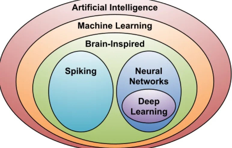
DNNs are the realization of the concept of deep learning, which is a part of the broader field of AI as shown in Fig. 1-1. They are inspired by how biological nervous systems communicate and process information. In a DNN, the raw sensory input data is hierarchically transformed, either in time or space, into high-level abstract representations in order to extract useful information. This transformation, called inference, involves multiple stages

(21)

Artificial Intelligence Machine Learning Brain-Inspired Spiking Neural Networks Deep Learning

Figure 1-1: The various branches in the field of artificial intelligence.

Neurons (activations)

Synapses (weights)

(a) Neurons and synapses

X1 X2 X3 Y1 Y2 Y3 Y4 W11 W34 L1 Input Neurons (e.g. image pixels)

Layer 1

L1 Output Neurons a.k.a. Activations

Layer 2

L2 Output Neurons

(b) Compute weighted sums for each layer

Figure 1-2: A simple neural network example and terminology (Figures adopted from [41]). of non-linear processing, each of which is often referred to as a layer. Fig. 1-2 shows an example of a simple neural network with 2 layers, and a DNN often has from dozens to even thousands of layers. Each DNN layer performs a weighted sum of the input values, called input activations, followed by an non-linear function (e.g., sigmoid, hyperbolic tangent, or the rectified linear unit (ReLU) [48]) as shown in Fig. 1-3. The weights of each layer are determined through a process called training. In this thesis, we will focus on the use of the trained model, which is called inference.

DNNs come in a wide variety of configurations in both the types of layer and their shapes and sizes. They are also evolving rapidly with improved accuracy and hardware performance.

(22)

yj= f wixi i

∑

+ b ⎛ ⎝ ⎜ ⎞ ⎠ ⎟ w1x1 w2x2 w0x0 x0 w0 synapse axon dendrite axon neuron yj

Figure 1-3: The weighted sum in a neuron. xi, wi, f (·), and b are the activations, weights,

non-linear function and bias, respectively (Figures adopted from [41]).

Despite the many options, there are two primary types of layers that are indispensible in most DNNs: the convolutional (CONV) layer and fully-connected (FC) layer. DNNs that are composed solely of FC layers are also referred to as multi-layer perceptrons (MLP), while DNNs that contain CONV layers are called convolutional neural networks (CNNs).

The processing of both the CONV and FC layers can be described as performing high-dimensional convolutions as shown in Fig. 1-4. In this computation, the input activations of a layer are structured as a set of 2-D input feature maps (fmaps), each of which is called a channel. Each channel is convolved with a distinct 2-D filter from the stack of filters, one for each channel; this stack of 2-D filters is often referred to as a single 3-D filter. The intermediate values generated by the many 2-D convolutions for each output activation, called partial sums (psums), are then summed across all of the channels. In addition, a 1-D bias can be added to the filtering results, but some recent networks [28] remove its usage from parts of the layers. The results of this computation are the output activations that comprise one channel of output feature map. Additional 3-D filters can be used on the same input fmaps to create additional output channels. Finally, multiple input fmaps may be processed together as a batch to potentially improve reuse of the filter weights.

(23)

Input fmaps

Filters Output fmaps

R S C

…

H W C

…

E F M E F M

…

R S C H W C

1 N

1 M

1 N

Figure 1-4: The high-dimensional convolution performed in a CONV or FC layer of a DNN.

Given the shape parameters in Table 1.1, the computation of a CONV layer is defined as O[g][n][m][y][x] = B[g][m] + C−1

∑

c=0 R−1

∑

i=0 S−1

∑

j=0

I[g][n][c][U y + i][U x + j] × W[g][m][c][i][ j], 0 ≤ g < G, 0 ≤ n < N, 0 ≤ m < M, 0 ≤ x < F, 0 ≤ y < E,

E= (H − R +U )/U, F = (W − S +U )/U.

(1.1) O, I, W and B are the matrices of the output fmaps, input fmaps, filters and biases, respec-tively. U is a given stride size. For FC layers, Eq. (1.1) still holds with a few additional constraints on the shape parameters: H = R, F = S, E = F = 1, and U = 1. Fig. 1-4 shows a visualization of this computation (ignoring biases) assuming G = 1, and Fig. 1-5 shows an naive loop nest implementation of this computation.

(24)

Shape Parameter Description

G number of convolution groups N batch size of 3-D fmaps

M # of 3-D filters / # of output channels C # of input channels

H/W input fmap plane height/width

R/S filter plane height/width (= H or W in FC) E/F output fmap plane height/width (= 1 in FC) Table 1.1: Shape parameters of a CONV/FC layer.

Input Fmaps: I[G][N][C][H][W] Filter Weights: W[G][M][C][R][S] Biases: B[G][M] Output Fmaps: O[G][N][M][E][F] for (g=0; g<G; g++) { for (n=0; n<N; n++) { for (m=0; m<M; m++) { for (x=0; x<F; x++) { for (y=0; y<E; y++) { O[g][n][m][y][x] = B[g][m]; for (j=0; j<S; j++) { for (i=0; i<R; i++) { for (k=0; k<C; k++) { O[g][n][m][y][x] += I[g][n][k][Uy+i][Ux+j] × W[g][m][k][i][j]; }}}}}}}}

Figure 1-5: A naive loop nest implementation of the high-dimensional convolution in Eq. (1.1).

1.1.2 Challenges in DNN processing

In most of the widely used DNNs, the multiply-and-accumulate (MAC) operations in the CONV and FC layers account for over 99% of the overall operations. Not only is the amount of operations high, which can go up to several hundred millions of MACs per layer, they also generate a large amount of data movement. Therefore, they have a significant impact on the processing throughput and energy efficiency of DNNs. Specifically, they pose two challenges: data handling and adaptive processing. The details of each are described below. Data Handling: Although the MAC operations in Eq. (1.1) can run at high parallelism, which greatly benefits throughput, it also creates two issues. First, naïvely reading inputs for all MACs directly from DRAM requires high bandwidth and incurs high energy consumption.

(25)

Filter Reuse

Convolutional Reuse Fmap Reuse

CONV layers only

(sliding window) CONV and FC layers CONV and FC layers (batch size > 1)

Filter Input Fmap

Filters 2 1 Input Fmap Filter 2 1 Input Fmaps Activations Filter weights

Reuse: Reuse: Activations Reuse: Filter weights

Figure 1-6: Data reuse opportunities in a CONV or FC layers of DNNs [7].

Second, a significant amount of intermediate data, i.e., psums, is generated by the parallel MACs simultaneously, which poses storage pressure and consumes additional memory read and write energy if not processed, i.e., accumulated, immediately.

Fortunately, the first issue can be alleviated by exploiting different types of input data reuseas shown in Fig. 1-6:

∙ convolutional reuse: Due to the weight sharing property in CONV layers, a small amount of unique input activations can be shared across many operations. Each filter weight is reused E2times in the same input fmap plane, and each input activation is usually reused R2times in the same filter plane. FC layers, however, do not have this type of data reuse.

∙ filter reuse: Each filter weight is further reused across the batch of N input fmaps in both CONV and FC layers.

∙ fmap reuse: Each input activation is further reused across M filters (to generate the Moutput channels) in both CONV and FC layers.

(26)

Layer H1 R/S E/F G C M U CONV1 227 11 55 1 3 96 4 CONV2 31 5 27 2 48 256 1 CONV3 15 3 13 1 256 384 1 CONV4 15 3 13 2 192 384 1 CONV5 15 3 13 2 192 256 1 FC1 6 6 1 1 256 4096 1 FC2 1 1 1 1 4096 4096 1 FC3 1 1 1 1 4096 1000 1

1 _{This is the padded size}

Table 1.2: CONV/FC layer shape configurations in AlexNet [34].

psums can be reduced as soon as possible to save both the storage space and memory read and write energy. CR2psums are reduced into one output activation.

Unfortunately, maximum input data reuse cannot be achieved simultaneously with immediate psum reduction, since the psums generated by MACs using the same weight or input activation are not reducible. In order to achieve high throughput and energy efficiency, the underlying DNN dataflow, which dictates how the MAC operations are scheduled for processing (Chapter 2 will provide a more formal definition of a dataflow), needs to account for both input data reuse and psum accumulation scheduling at the same time.

Adaptive Processing: The many shape parameters shown in Table 1.1 give rise to many possible CONV and FC layer shapes. Even within the same DNN model, each layer can have distinct shape configurations. Table 1.2 shows the shape configurations of AlexNet [36] as an example. The hardware architecture, therefore, cannot be hardwired to process only certain shapes. Instead, the dataflow must be efficient for different shapes, and the hardware architecture must be programmable to dynamically map to an efficient dataflow.

1.1.3 DNN vs. Conventional Digital Signal Processing

Before DNNs became mainstream, there was already research on high-efficiency and high-performance digital signal processing. For example, convolution processors have a wide applicability in image signal processing (ISP) [55]; linear algebra libraries, such as ATLAS [69], have also been used extensively across many fields. They have proposed

(27)

many optimization techniques, including tiling strategies used in multiprocessors and SIMD instructions, to perform convolution or matrix multiplication at high performance on various compute platforms. While many of these techniques can be applied for DNN processing, they do not directly optimize for the best performance and energy efficiency for the following reasons:

∙ The filter weights in DNNs are obtained through training instead of fixed in the processing system. Therefore, they can consume significant I/O bandwidth and on-chip storage, sometimes comparable to that of the input fmaps.

∙ Lowering the high-dimensional convolution into matrix multiplication also loses the opportunities to optimize for convolutional data reuse, which can be the key to achieving high energy efficiency.

∙ The ISP techniques are developed mainly for 2D convolutions. They do not opti-mize processing resources for data reuse nor do they address the non-trivial psum accumulation in DNN.

1.2 Spatial Architecture

Spatial architectures are a class of accelerators that can exploit high compute parallelism using direct communication between an array of relatively simple processing engines (PEs). They can be designed or programmed to support different algorithms, which are mapped onto the PEs using specialized dataflows. Compared with SIMD/SIMT architectures, spatial architectures are particularly suitable for applications whose dataflow exhibits producer-consumer relationships or can leverage efficient data sharing among a region of PEs.

Spatial architectures come in two flavors: coarse-grained spatial architectures that consist of tiled arrays of ALU-style PEs connected together via on-chip networks [27, 44, 46], and fine-grained spatial architectures that are usually in the form of an FPGA. The expected performance advantage and large design space of coarse-grained spatial architectures has inspired much research on the evaluation of its architectures, control schemes, operation scheduling and dataflow models [2, 22, 49, 51, 58, 63].

(28)

PE Array

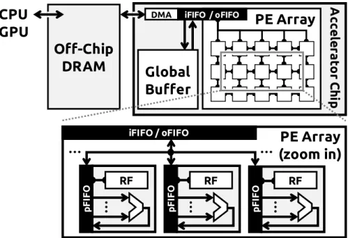
(zoom in)

pF IF O RF RF pF IF O RF pF IF O iFIFO / oFIFO … …

Global

Buffer

PE Array

iFIFO / oFIFO

Off-Chip

DRAM

A cce le ra to r C h ip

CPU

GPU

… … … DMA

Figure 1-7: Block diagram of a general DNN accelerator system consisting of a spatial architecture accelerator and an off-chip DRAM. The zoom-in shows the high-level structure of a processing element (PE).

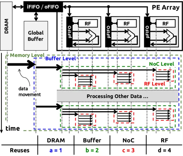
Coarse-grained spatial architectures are currently a very popular implementation choice for specialized DNN accelerators for two reasons. First, the operations in a DNN layer are uniform and exhibit high parallelism, which can be computed quite naturally with parallel ALU-style PEs. Second, direct inter-PE communication can be used very effectively for (1) passing partial sums to achieve spatially distributed accumulation, or (2) sharing the same input data for parallel computation without incurring higher energy data transfers. Third, the multi-level storage hierarchy provides many inexpensive ways for data access to exploit data reuse. ASIC implementations usually deploy dozens to hundreds of PEs and specialize the PE datapath only for DNN computation [3, 5, 13, 18, 53]. FPGAs are also used to build DNN accelerators, and these designs usually use integrated DSP slices to construct the PE datapaths [4, 20, 23, 54, 57, 62, 74]. However, the challenge in either type of design lies in the exact mapping of the DNN dataflow to the spatial architecture, since it has a strong impact on the resulting throughput and energy efficiency.

Fig. 1-7 illustrates the high-level block diagram of the accelerator system that is used in this thesis for DNN processing. It consists of a spatial architecture accelerator and off-chip

(29)

DRAM. The inputs can be off-loaded from the CPU or GPU to DRAM and processed by the accelerator. The outputs are then written back to DRAM and further interpreted by the main processor.

The spatial architecture accelerator is primarily composed of a global buffer (GLB) and an array of PEs. The DRAM, global buffer and PE array communicate with each other through the input and output FIFOs (iFIFO/oFIFO). The global buffer can be used to exploit input data reuse and hide DRAM access latency, or for the storage of intermediate data. Currently, the typical size of the global buffer used for DNN acceleration is around several hundred kB to a few MB. The PEs in the array are connected via an on-chip network (NoC), and the NoC design depends on the dataflow requirements. The PE includes an ALU datapath, which is capable of doing MAC and addition, a register file (RF) as a local scratchpad (SPad), and a PE FIFO (pFIFO) used to control the traffic going in and out of the ALU. Different dataflows require a wide range of RF sizes, ranging from zero to a few hundred bytes. Typical RF size is below 1kB per PE. Overall, the system provides four levels of storage hierarchy for data accesses, including DRAM, global buffer, NoC (inter-PE communication) and RF. Accessing data from a different level also implies a different energy cost, with the highest cost at DRAM and the lowest cost at RF.

1.3 Related Work

There is currently a large amount of work on the acceleration of DNN processing for various compute platforms, and it is still growing rapidly given the popularity of the research field. Therefore, this section serves to provide a taste of the breadth of research in this field with a representative list of related previous work.

First of all, there is a wide range of proposed architectures for DNN acceleration [3, 4, 5, 13, 18, 20, 23, 35, 47, 50, 53, 54, 57, 60, 62, 73, 74]. While many of them can be described as based on a spatial architecture, it is usually very hard to analyze and compare them due to the following reasons. First, they are often implemented or simulated with different process technologies and available hardware resources. Second, many of them do not report the performance and/or energy efficiency based on publicly available benchmarks. In order

(30)

to fairly compare different architectures, we propose (1) a taxonomy of DNN processing dataflows that can capture the essence of how different architectures perform the processing (Chapter 2), and (2) analysis methodologies that can quantify the impact of various dataflows on energy efficiency (Section 3.2). We will then introduce a novel dataflow, called Row Stationary (RS), that can optimize for the overall energy efficiency of the system for vairous DNN shapes and sizes in Chapter 3.

In addition to the analysis on energy efficiency, performance modeling is also a critical part in the design of DNN accelerators. Chen et al. [74] explore various optimization techniques, such as loop tiling and transformation, to map a DNN workload onto an FPGA, and then uses a roofline model [70] of the charateristics of the FPGA to identify the solution with best performance and lowest resource requirements. Jouppi et al. [35] also use a roofline model to illustrate the impact of limited bandwidth on performance. In this work, we propose a method called Eyexam to tighten the bounds of the roofline model based on the various architectural design choices and their interaction with the given DNN workload. We also adapt the roofline model for DNN processing by accounting for the fact that different data types (i.e., input activations, weight and psums) will have different bandwidth requirements and thus require three separate roofline models. These techniques will also be discussed in Section 5.2.

As the development of DNNs evolve, many DNN accelerators also start to take advantage of certain properties of the DNN [12]. For example, the activations exhibit a certain degree of sparsity thanks to the ReLU function; also, weight pruning has been shown as an effective method to further reduce the size and computation of a DNN [25, 26]. As a result, architectures such as EIE [24], CNVLUTIN [1] and SCNN [52] have been proposed to take advantage of data sparsity to improve processing throughput and energy efficiency. In Chapter 4 and Chapter 6, we will also discuss how the Eyeriss architecture can exploit data sparsity.

Finally, as we will describe in Chapter 5, the requirement for flexibility has been increasing due to the more diverse set of DNNs proposed in recent years. Previous work that explored flexible hardware for DNNs include FlexFlow [42], DNA [68] and Maeri [38], which propose methods to support multiple dataflows within the same NoC. Rather than

(31)

supporting multiple dataflows, Eyeriss proposes using a single but highly flexible dataflow. Along with a highly flexible NoC that can adapt to a wide range of bandwidth requirements while still being able to exploit available data reuse, they can efficiently support a wide range of layer shapes to maximize the number of active PEs and keep the PEs busy for high performance.

1.4 Thesis Contributions

In this thesis, we demonstrate how to optimize for performance and energy efficiency in the processing of a wide range of DNNs. While the processing can benefit from highly-parallel architectures to achieve high throughput, the computation requires a large amount of data, which involves significant data movement that has become the bottleneck of both performance and energy efficiency [14, 29]. To address this issue, the key is to find a dataflowthat can fully exploit data reuse in the local memory hierarchy and parallelism to minimize accesses to the high-cost memory levels, such as DRAM. The dataflow has to perform this optimization for a wide range of DNN shapes and sizes. In addition, it also has to fully utilize the parallelism to achieve high performance.

1.4.1 Dataflow Taxonomy

Numerous previous efforts have proposed solutions for DNN acceleration. These designs reflect a variety of trade-offs between performance, energy efficiency and implementation complexity. Though with their differences in low-level implementation details, we find that many of them can be described as embodying a set of dataflows. As a result, we are able to classify them into a taxonomy of four dataflow categories. Comparing different implementations in terms of dataflow provides a more objective view of the architecture, and makes it easier to isolate specific contributions in individual designs. This work is discussed in Chapter 2 and appears in [7, 8].

(32)

1.4.2 Energy and Performance Analysis Methodologies

We developed methodologies to systematically analyze the energy efficiency and perfor-mance of any architectures for DNN processing. They provide a fast way to assess an architecture by examining how the underlying dataflow exploits data reuse in a memory hier-archy and parallelism and how the hardware supports the dataflow. Through these analyses, we have identified certain properties that are critical to the design of DNN accelerators. For example, optimizing for the data reuse of a certain data type does not necessarily translate to the best overall system energy efficiency. Also, to support a diverse set of DNNs, the hardware has to be able to adapt to a wide range of data reuse; otherwise, it can result in low utilization of the parallelism or insufficient data bandwidth to support the processing. We will address these issues in our proposed designs. The energy efficiency analysis framework is discussed in Section 3.2 and appears in [7]. The performance analysis framework is discussed in Section 5.2 in [9].

1.4.3 Energy-efficient Dataflow: Row-Stationary

While the existing dataflows in the taxonomy are popular among many implementations, they are designed to optimize the energy efficiency of accessing a certain data type or memory level in the hierarchy. We propose a new dataflow, called Row-Stationary (RS), that optimizes for the overall system energy efficiency directly by fully exploiting data reuse in a multi-level memory hierarchy for all data types while supporting highly-parallel computation for any given DNN shape and size. The RS dataflow poses the operation mapping process as an optimization problem instead of hand-crafting which data type or memory level should receive the most reuse within the limited hardware resources. It has shown up to 2.5× higher energy efficiency than other dataflows. This work is discussed in Chapter 3 and appears in [7].

1.4.4 Eyeriss v1 Architecture

We designed an architecture, named Eyeriss v1, to support the RS dataflow and further optimize the hardware for higher performance and energy efficiency. Eyeriss v1 targets large

(33)

DNN models, which have plenty of data reuse opportunities for optimization. In addition to the efficiency brought by the RS dataflow, Eyeriss v1 has the following features.

∙ It uses a flexible mapping strategy to turn the logical mapping in the RS dataflow, which is done regardless of the actual size of the processing element (PE) array in the hardware, into a mapping that fits in the physical dimensions of the PE array. This ensures as many PEs can be utilized as possible for higher performance.

∙ It uses a multicast on-chip network (NoC) to fully exploit data reuse when delivering data from the global buffer to the PEs. At the same time, the implementation of the multicast NoC shuts down unused data buses to reduce data traffic, which provides an over 80% energy savings over a broadcast NoC design.

∙ It further exploits the sparsity (zero data) in the feature maps to achieve higher energy efficiency. In particular, it utilizes a zero-skipping logic in the PE to reduce the switching activity of the circuits and the accesses to the register file when data is zero, and saves 45% of PE power. It also compresses the feature map data with a simple run-length coding, which reduces off-chip data bandwidth by 1.2× to 1.9×.

Eyeriss v1 was fabricated in a 65nm CMOS process, and can process the CONV layers of AlexNet at 34.7 fps while consuming 278 mW. The overall energy efficiency was 10× higher than a mobile GPU. We have further integrated the chip with the Caffe deep learning framework and demonstrated an image classification system to showcase the flexibility of the chip for supporting real-world applications. This work is discussed in Chapter 4 and appears in [10, 11].

1.4.5 Highly-Flexible Dataflow and On-Chip Network

The recent trend of DNN development has an increasing focus on reducing the size and computation complexity of DNNs. However, this also results in a higher variation in the amount of data reuse. Many of the existing DNN accelerators were designed for DNNs with plenty of data reuse. As a result, they cannot adapt well to emerging DNNs and therefore lose performance. To solve this problem, we propose two architectural improvements:

(34)

∙ a flexible dataflow, named RS Plus (RS+), that inherits the capability of the RS dataflow to optimize for overall energy efficiency and further improves the utilization of PEs when data reuse is low by being able to parallelize the computation in any dimensions of the data.

∙ a flexible and scalable hierarchical mesh NoC that can provide high bandwidth when data reuse is low while still being able to exploit high data reuse when available. Together, they increase the utilization of the PEs in terms of both the number of active PEs and the percentage of active cycles for each PE. Overall, they provide a throughput speedup of over 10× than Eyeriss v1 at 256 PEs, and the performance advantage goes higher when the architecture scales (i.e., increase number of PEs). This work is discussed in Chapter 5 and appears in [12].

1.4.6 Eyeriss v2 Architecture

Eyeriss v2 is designed to support the RS+ dataflow and the hierarchical mesh NoC. In addition, it has the following features:

∙ it exploits data sparsity to not only improve energy efficiency, but also the processing throughput. This is done by processing data directly in a compressed format for both the feature maps and weights. When data sparsity is low, however, it can still adapt back to process data in the raw format so it does not introduce overhead in the data movement due to compression.

∙ it introduces SIMD processing in each PE by having two MAC datapaths instead of one. This improves not only throughput but also energy efficiency due to the amortized cost of the memory control logic.

These additional features can bring an additional 6× speedup in throughput. Overall, Eyeriss v2 achieves a speedup of 40× and 10× with 11.3× and 1.9× higher energy efficiency on AlexNet and MobileNet, respectively, over Eyeriss v1 even at the batch size of 1. This work is discussed in Chapter 6 and appears in [12].

(35)

Chapter 2 DNN Processing Dataflows

2.1 Definition

The high-dimensional convolutions in DNNs involve a significant amount of MAC op-erations, which also generate a significant amount of data movement. As described in Section 1.1.2, the challenges in processing are threefold. First of all, the accelerator has to parallelize the MAC operations so that they efficiently utilize the available compute re-sources in the hardware for high performance. Second, the operations have to be scheduled in a way that can exploit data reuse in a multi-level storage hierarchy, such as the ones introduced in the spatial architecture, in order to minimize data movement for high energy efficiency. This is done by maximizing the reuse of data in the lower-energy-cost storage levels, e.g., local RF, thus minimizing data accesses to the higher-cost levels, e.g., DRAM. Finally, the hardware has to adapt to a wide range of DNN configurations.

These challenges can be framed as an optimization process that finds the optimal MAC operation mapping on the hardware architecture for processing. For each MAC operation in a DNN, which is uniquely defined by its associated input activation, weight and psum, the mapping determines its temporal scheduling (in which cycle it is executed) and spatial scheduling (in which PE it is executed) on a highly-parallel architecture. In a mapping optimized for energy efficiency, data in the lower-cost storage levels can be reused by as many MACs as possible before replacement. However, due to the limited amount of local storage, input data reuse (for activations and weights) and local psum accumulation cannot

(36)

be fully exploited simultaneously. Therefore, the system energy efficiency is maximized only when the mapping balances all types of data reuse in a multi-level storage hierarchy. In a mapping optimized for throughput, as many PEs will be active for processing for as many cycles as possible, thus minimizing idle compute resources. These two objectives can be further combined to find the mapping that meets a balance of both constraints.

This optimization has to take into account the following two factors: (1) the shape and size of the DNN layer, e.g., number of filters, number of channels, size of filters, etc, which determine the data reuse opportunities, and (2) the available processing parallelism, the storage capacity and the associated energy cost of data access at each level of the memory hierarchy, which are a function of the specific accelerator implementation. Therefore, the optimal mapping changes across different DNN layers as well as hardware configurations. Due to implementation trade-offs, a specific DNN accelerator design can only find the optimal mapping from the subset of supported mappings instead of the entire mapping space. The subset of supported mappings is usually determined by a set of mapping rules, which also characterizes the hardware implementation. For example, in order to simplify the data delivery from the global buffer to the PE array, the mapping may only allow all parallel MACs to execute on the same weight in order to take advantage of a broadcast NoC design, which sacrifices flexibility for efficiency.

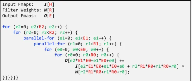
We define the set of mapping rules as a dataflow that can be described by a loop nest with pre-defined loop orders and variable loop limits. For simplicity, Fig. 2-1 shows an example dataflow for a 1D convolution between an 1D input fmap of size H and 1D filter of size R, which generates an 1D output fmap of size E. The ordering and parallelization of the for-loops determine the rules for the temporal and spatial scheduling of the MAC operations, respectively. The limit of each loop, e.g., E2, E1, E0, R2, R1, R0, where E = E2 × E1 × E0, R = R2 × R1 × R0, however, does not have to be determined by the dataflow. This provides flexibility in the dataflow. For example, when R0 = R (and R1 = 1 and R2 = 1), the processing goes through all weights in the inner-most loop, while when R2 = R (and R0 = 1 and R1 = 1), the weight stays the same in the inner-most loop. This flexibility creates the supported mapping space for the optimization process to find the optimal mapping for a given objective.

(37)

Input Fmaps: I[H] Filter Weights: W[R] Output Fmaps: O[E] for (e2=0; e2<E2; e2++) { for (r2=0; r2<R2; r2++) { parallel-for (e1=0; e1<E1; e1++) { parallel-for (r1=0; r1<R1; r1++) { for (e0=0; e0<E0; e0++) { for (r0=0; r0<R0; r0++) { O[e2*E1*E0+e1*E0+e0] += I[e2*E1*E0+e1*E0+e0 + r2*R1*R0+r1*R0+r0] × W[r2*R1*R0+r1*R0+r0]; }}}}}}

Figure 2-1: An example dataflow for a 1D convolution.

A mapping is generated by determining the loop limits in a given dataflow, which is a process called tiling that is a part of the optimization. Tiling has to take into account not only the shape and size of the data, i.e., H, R and E in the example of Fig. 2-1, but also hardware resources such as the number of PEs, the number of levels in the memory hierarchy and the storage size at each memory level. For example, when only 8 PEs are available, it imposes the following constraint: E1 × R1 ≤ 8.

The design of a DNN accelerator architecture starts with the design of the dataflow, and an architecture can be designed to support multiple dataflows at once, which brings the potential advantage of a larger mapping space for optimization. However, there is usually a trade-off between the flexibility and efficiency of the architecture. Since there exists a large number of potential dataflows, it creates an enormous design space for exploration.

2.2 An Analogy to General-Purpose Processors

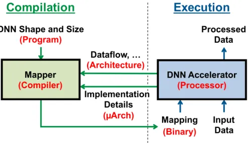
The operation of DNN accelerators is analogous to that of general-purpose processors as illustrated in Fig. 2-2. In conventional computer systems, the compiler translates the program into machine-readable binary codes for execution; in the processing of DNNs, the mapper translates the DNN shape and size into a hardware-compatible mapping for execution.

(38)

Compilation

Execution

DNN Shape and Size (Program) Mapping Input Data Processed Data Mapper (Compiler) DNN Accelerator (Processor) Dataflow, … (Architecture) (Binary) Implementation Details (µArch)

Figure 2-2: An analogy between the operation of DNN accelerators (texts in black) and that of general-purpose processors (texts in red).

processor. Similar to the role of an ISA or memory consistency model, dataflow characterizes the hardware implementation and defines the mapping rules that the mapper has to follow in order to generate hardware-compatible mappings. We consider the dataflow as a part of the architecture, instead of microarchitecture, since we believe it is going to largely remain invariant across implementations. Although, similar to GPUs, the distinction between architecture and microarchitecture is likely to blur for DNN accelerators due to its rapid development. In Section 2.3, we will introduce several existing dataflows that are widely used in implementations.

The hardware implementation details, such as the degree of pipelining in the PE or the bandwidth of NoC for data delivery, are analogous to the microarchitecture of processors for the following reasons: (1) they can vary a lot across implementations, and (2) although they can play a vital part in the optimization, they are not essential since the mapper can always generate sub-optimal mappings.

The goal of the mapper is to search in the mapping space for the best one that optimizes data movement and/or PE utilization. The size of the entire mapping space is determined by the total number of MACs, which can be calculated from the DNN shape and size. However, only a subset of the space is valid given the mapping rules defined by a dataflow. It is the

(39)

mapper’s job to find out the exact ordering of these MACs on each PE by evaluating and comparing different valid ordering options based on the optimization objective.

As in conventional compilers, performing evaluation is an integral part of the mapper. The evaluation process takes a certain mapping as input and gives an energy consumption and performance estimation based on the available hardware resources (microarchitecture) and the data size and reuse opportunities extracted from the DNN configuration (program). In Section 3.2 and 5.2, we will introduce frameworks that can perform this evaluation.

2.3 A Taxonomy of Existing DNN Dataflows

For computer architects, trade-offs between performance, energy-efficiency and implemen-tation complexity are always of primary concern in architecture designs. This is the same case for designing DNN dataflows. On the one hand, if the dataflow accommodates a large number of valid operation mappings, the mapper has a better chance to find the one with optimal energy efficiency. On the other hand, however, the complexity and cost of hardware implementations might be too high to support such a dataflow, which makes it of no practical use. Therefore, it is very important to identify dataflows that have a strong root in implementation.

Numerous previous efforts have proposed solutions for DNN acceleration. These designs reflect a variety of trade-offs between performance, energy efficiency and implementation complexity. Though with their differences in low-level implementation details, we find that many of them can be described as embodying a set of rules, i.e., dataflow, that define the valid mapping space based on how they handle data. As a result, we are able to classify them into a taxonomy of four dataflow categories. In the rest of this section, we will provide a high-level overview on each of the four dataflows.

∙ Weight-Stationary (WS) dataflow: WS keeps filter weights stationary in the RF of each PE by enforcing the following mapping rule: all MACs that use the same filter weight have to be mapped on the same PE for processing contiguously. This maximizes the convolutional and filter reuse of weights in the RF, thus minimizing the energy consumption of accessing weights (e.g., [3, 4, 20, 35, 53]). Fig. 2-3a shows the

(40)

data movement of a common WS dataflow implementation. While each weight stays in the RF of each PE, unique input activations are sent to each PE, and the generated psums are then accumulated spatially across PEs.

∙ Output-Stationary (OS) dataflow: OS keeps psums stationary by accumulating them locally in the RF. The mapping rule is: all MACs that generate psums for the same ofmap pixel have to be mapped on the same PE contiguously. This maximizes psum reuse in the RF, thus minimizing energy consumption of psum movement (e.g., [18, 23, 47, 54, 73]). The data movement of a common OS dataflow implementa-tion is to broadcast filter weights while passing unique input activaimplementa-tions to each PE (Fig. 2-3b).

∙ Input-Stationary (IS) dataflow: IS keeps input activations stationary in the RF of each PE by enforcing the following mapping rule: all MACs that use the same input activation have to be mapped on the same PE for processing contiguously. This maximizes the convolutional and fmap reuse of input activations in the RF, thus minimizing the energy consumption of accessing input activations (e.g., [52]). In addition to keeping input activations stationary in the RF, a common IS dataflow implementation is to send unique weights to each PE, and the generated psums are then accumulated spatially across PEs (Fig. 2-3c).

∙ No Local Reuse (NLR) dataflow: Unlike the previous dataflows that keep a certain data type stationary, NLR makes no data stationary locally so it can trade RF off for a large global buffer. This is to minimize DRAM access energy consumption by storing more data on-chip (e.g., [5, 74]). The corresponding mapping rule is: at each processing cycle, all parallel MACs correspond to an unique pair of input channel (for input activation and weight) and output channel (for psum). The data movement of NLR dataflow is to single-cast weights, multi-cast ifmap pixels, and spatially accumulate psums across the PE array (Fig. 2-3d).

The four dataflows show distinct data movement patterns, which imply different trade-offs. First, as is evident in Fig. 2-3a, Fig. 2-3b and Fig. 2-3c, the cost for keeping a specific

(41)

data type stationary is to move the other types of data more. Second, the timing of data accesses also matters. For example, in the OS dataflow, each weight read from the global buffer is broadcast to all PEs with properly mapped MACs on the PE array. This is more efficient than reading the same value multiple times from the global buffer and single-casting it to the PEs, which is the case for filter weights in the NLR dataflow (Fig. 2-3d) due to its mapping restriction. In Chapter 3, we will present a new dataflow that takes these factors into account to optimized for energy efficiency.

2.4 Conclusions

Dataflow is an integral part in the design of DNN accelerators. It dictates the performance and energy efficiency of the hardware, and is a key attribute of the accelerator that is analogous to the architecture of a general-purpose processor. Based on this insight, we find that many of the existing DNN accelerator architectures can be classified into a taxonomy of four dataflows. However, we also notice that these existing dataflows only optimize for the energy efficiency of certain data types or specific levels of memory hierarchy instead of for the overall system energy efficiency. In Chapter 3, we will introduce a new dataflow, called row-stationary, that can achieve this goal.

(42)

Global Buffer

W0 W1 W2 W3 W4 W5 W6 W7

Psum

Act

PE

Weight

(a) Weight-Stationary (WS) Dataflow

Global Buffer

Act

Weight

PE

Psum

P0 P1 P2 P3 P4 P5 P6 P7

(b) Output-Stationary (OS) Dataflow

Global Buffer

I0 I1 I2 I3 I4 I5 I6 I7

Psum

Act PE

Weight

(c) Input-Stationary (IS) dataflow

PE

Act

Psum

Global Buffer

Weight

(d) No Local Reuse (NLR) dataflow

(43)

Chapter 3 Energy-Efficient Dataflow:

Row-Stationary

3.1 How Row-Stationary Works

While existing dataflows attempt to maximize certain types of input data reuse or minimize the psum accumulation cost, they fail to take all of them into account at once. This results in inefficiency when the layer shape or hardware resources vary. Therefore, it would be desirable if the dataflow could adapt to different conditions and optimize for all types of data movement energy costs. In this chapter, we will introduce a novel dataflow, called row stationary(RS) that achieves this goal.

3.1.1 1D Convolution Primitives

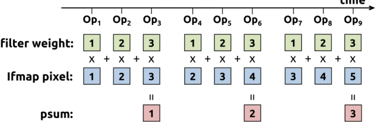
The implementation of the RS dataflow in Eyeriss is inspired by the idea of applying a strip mining technique in a spatial architecture [67]. It breaks the high-dimensional convolution down into 1D convolution primitives that can run in parallel; each primitive operates on one row of filter weights and one row of ifmap pixels, and generates one row of psums. Psums from different primitives are further accumulated together to generate the ofmap pixels. The inputs to the 1D convolution come from the storage hierarchy, e.g., the global buffer or DRAM.

(44)

time 1 2 3 1 2 3 x + x + x = 1 Op1 Op2 Op3 1 2 3 2 3 4 x + x + x = 2 Op4 Op5 Op6 1 2 3 3 4 5 x + x + x = 3 Op7 Op8 Op9 filter weight: Ifmap pixel: psum:

Figure 3-1: Processing of an 1D convolution primitive in the PE. In this example, R = 3 and H = 5.

Each primitive is mapped to one PE for processing; therefore, the computation of each row pair stays stationaryin the PE, which creates convolutional reuse of filter weights and ifmap pixels at the RF level. An example of this sliding window processing is shown in Fig. 3-1. However, since the entire convolution usually contains hundreds of thousands of primitives, the exact mapping of all primitives to the PE array is non-trivial, and will greatly affect the energy efficiency.

3.1.2 Two-Step Primitive Mapping

To solve this problem, the primitive mapping is separated into two steps: logical mapping and physical mapping. The logical mapping first deploys the primitives into a logical PE array, which has the same size as the number of 1D convolution primitives and is usually much larger than the physical PE array in hardware. The physical mapping then folds the logical PE array so it fits into the physical PE array. Folding implies serializing the computation, and is determined by the amount of on-chip storage, including both the global buffer and local RF. The two mapping steps happen statically prior to runtime, so no on-line computation is required.

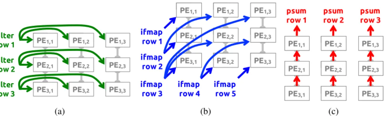
Logical Mapping: Each 1D primitive is first mapped to one logical PE in the logical PE array. Since there is considerable spatial locality between the PEs that compute a 2D convolution in the logical PE array, we group them together as a logical PE set. Fig. 3-2 shows a logical PE set, where each filter row and ifmap row are horizontally and diagonally

(45)

PE1,1 PE1,2 PE1,3 filter row 1 PE2,1 PE2,2 PE2,3 filter row 2 PE3,1 PE3,2 PE3,3 filter row 3 (a) PE1,1 PE1,2 PE1,3 ifmap row 1 PE2,1 PE2,2 PE2,3 ifmap row 2 PE3,1 PE3,2 PE3,3 ifmap row 3 ifmap row 4 ifmap row 5 (b) PE1,3 PE2,3 PE3,3 psum row 3 PE1,2 PE2,2 PE3,2 psum row 2 PE1,1 psum row 1 PE2,1 PE3,1 (c)

Figure 3-2: The dataflow in a logical PE set to process a 2D convolution. (a) rows of filter weight are reused across PEs horizontally. (b) rows of ifmap pixel are reused across PEs diagonally. (c) rows of psum are accumulated across PEs vertically. In this example, R = 3 and H = 5.

reused, respectively, and each row of psums is vertically accumulated. The height and width of a logical PE set are determined by the filter height (R) and ofmap height (E), respectively. Since the number of 2D convolutions in a CONV layer is equal to the product of number of ifmap/filter channels (C), number of filters (M) and fmap batch size (N), the logical PE array requires N × M ×C logical PE sets to complete the processing of an entire CONV layer. Physical Mapping: Folding means mapping and then running multiple 1D convolution primitives from different logical PEs on the same physical PE. In the RS dataflow, folding is done at the granularity of logical PE sets for two reasons. First, it preserves intra-set convolutional reuse and psum accumulation at the array level (inter-PE communication) as shown in Fig. 3-2. Second, there exists more data reuse and psum accumulation opportunities across the N × M ×C sets: the same filter weights can be shared across N sets (filter reuse), the same ifmap pixels can be shared across M sets (ifmap reuse), and the psums across each Csets can be accumulated together. Folding multiple logical PEs from the same position of different sets onto a single physical PE exploits input data reuse and psum accumulation at the RF level; the corresponding 1D convolution primitives run on the same physical PE in an interleaved fashion. Mapping multiple sets spatially across the physical PE array also exploits those opportunities at the array level. The exact amount of logical PE sets to fold and to map spatially at each of the three dimensions, i.e., N, M, and C, are determined by the RF size and physical PE array size, respectively. It then becomes an optimization problem to determine the best folding by using the framework in Section 3.2 to evaluate the results.

Architecture design for highly flexible and energy-efficient deep neural network accelerators

Architecture Design for Highly Flexible and

Energy-Efficient Deep Neural Network Accelerators

by

Yu-Hsin Chen

B.S. in EE, National Taiwan University (2009)

S.M. in EECS, Massachusetts Institute of Technology (2013)

Submitted to the

Department of Electrical Engineering and Computer Science

in partial fulfillment of the requirements for the degree of

Doctor of Philosophy

at the

MASSACHUSETTS INSTITUTE OF TECHNOLOGY

June 2018

c

○ Massachusetts Institute of Technology 2018. All rights reserved.

Author . . . .

Department of Electrical Engineering and Computer Science

May 23, 2018

Certified by . . . .

Vivienne Sze

Associate Professor of Electrical Engineering and Computer Science

Thesis Supervisor

Certified by . . . .

Joel Emer

Professor of Electrical Engineering and Computer Science

Thesis Supervisor

Accepted by . . . .

Leslie A. Kolodziejski

Professor of Electrical Engineering and Computer Science

Chairman, Department Committee on Graduate Theses

Architecture Design for Highly Flexible and

Energy-Efficient Deep Neural Network Accelerators

by

Yu-Hsin Chen

Abstract

Acknowledgments

Contents

List of Figures

List of Tables

Chapter 1

Introduction

1.1

Overview of Deep Neural Networks

1.1.1

The Basics

∑

…

…

…

1

N

1

M

1

N

∑

∑

∑

1.1.2

Challenges in DNN processing

1.1.3

DNN vs. Conventional Digital Signal Processing

1.2

Spatial Architecture

PE Array

(zoom in)

Global

Buffer

PE Array

Off-Chip

DRAM

CPU

GPU

1.3

Related Work

1.4

Thesis Contributions

1.4.1

Dataflow Taxonomy