HAL Id: hal-03155715
https://hal.archives-ouvertes.fr/hal-03155715
Preprint submitted on 2 Mar 2021
HAL is a multi-disciplinary open access
archive for the deposit and dissemination of
sci-entific research documents, whether they are
pub-lished or not. The documents may come from
teaching and research institutions in France or
abroad, or from public or private research centers.
L’archive ouverte pluridisciplinaire HAL, est
destinée au dépôt et à la diffusion de documents
scientifiques de niveau recherche, publiés ou non,
émanant des établissements d’enseignement et de
recherche français ou étrangers, des laboratoires
publics ou privés.
Normalization of series of fundus images to monitor the
geographic atrophy growth in dry age-related macular
degeneration
Florence Rossant, Michel Paques
To cite this version:
Florence Rossant, Michel Paques. Normalization of series of fundus images to monitor the geographic
atrophy growth in dry age-related macular degeneration. 2021. �hal-03155715�
1
Normalization of series of fundus images to monitor the geographic atrophy
growth in dry age-related macular degeneration
Corresponding author:
Florence ROSSANT, Professor,
Institut Supérieur d’Electronique de Paris (ISEP)
10, rue de Vanves, 92130 Issy-les-Moulineaux, France
Florence.rossant@isep.fr
33 1 49 54 52 62
Co-author :
Michel PAQUES, Professor
Clinical Investigation Center 1423, Quinze-Vingts Hospital, 28 rue de Charenton, Paris, France
mpaques@15-20.fr
1
Normalization of series of fundus images to monitor the geographic atrophy growth in
dry age-related macular degeneration
Florence
Rossant
a,and Michel
Paques
baISEP, Institut Supérieur d’Electronique de Paris, 10 rue de Vanves, 92130 Issy-les-Moulineaux, France, florence.rossant@isep.fr b Clinical Investigation Center 1423, Quinze-Vingts Hospital, 28 rue de Charenton, 75012 Paris, France
A B S T R A C T
Background and Objective: Age-related macular degeneration (ARMD) is a degenerative disease that affects the retina, and the leading cause of visual loss. In its dry form, the pathology is characterized by the progressive, centrifugal expansion of re tinal lesions, called geographic atrophy (GA). In infrared eye fundus images, the GA appears as localized bright areas and its growth can be observed in series of images acquired at regular time intervals. However, illumination distortions between the images make impossible the direct comparison of intensities in order to study the GA progress. Here, we propose a new method to compensate for illumination distortion between images.
Methods: We process all images of the series so that any two images have comparable gray levels. Our approach relies on an illumination/reflectance model. We first estimate the pixel-wise illumination ratio between any two images of the series, in a recursive way; then we correct each image against all the others, based on those estimates. The algorithm is applied on a sliding temporal window to cope with large changes in reflectance. We also propose morphological processing to suppress illumination artefacts.
Results: The corrected illumination function is homogeneous in the series, enabling the direct comparison of grey-levels intensities in each pixel, and so the detection of the GA growth between any two images. We present numerous experiments performed on a dataset of 18 series (328 images), manually segmented by an ophthalmologist. We demonstrate that the GA growth areas are better contrast after the proposed processing and we propose first segmentation methods to analyse the GA growth, with quantitative evaluation. Colored maps representing the GA evolution are derived from the segmentations.
Conclusion: To our knowledge, the proposed method is the first one which corrects automatically and jointly the illumination inhomogeneity in a series of fundus images, regardless of the number of images, the size, shape and progression of lesion areas. This algorithm greatly facilitates the visual interpretation by the medical expert. It opens up the possibility of treating automatically each series as a whole (not just in pairs of images) to model the GA growth.
Keywords – eye fundus images, normalization of series of images, dry age-related macular degeneration (ARMD), geographic atrophy (GA), GA progression detection, GA progression representation.
2
1. Introduction
Age-related macular degeneration (ARMD) is the leading cause of visual loss in our countries. It affects the retina, the photosensitive layer located in the back of the eye. While the so-called "wet" form of ARMD can be managed by a specific treatment, there is currently no therapeutic options for its "dry" form. The latter is characterized by the progressive, centrifugal expansion of retinal degeneration, giving rise to what has been compared to a geographic-like lesion, hence the name geographic atrophy (GA). The intimate mechanisms of the growth of the lesions remain elusive.
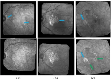
The diagnosis of ARMD is done on fundus photographs, of which many technical modalities are available. The disease is visible under the form of a localized change in the coloration of the fundus. Indeed, the affected layer is called the retinal pigment epithelium, which contains a pigment, melanin. Hence the disappearance of this layer causes a change in the coloration of the fundus, which can be observed most specifically in fundus imaging using long wavelengths such as red or infrared (IR) light (Fig. 1). This is why infrared imaging of the fundus through confocal scanning laser ophthalmoscopy (cSLO) is being widely used. This modality is comfortable for the patient, more robust and less invasive than fundus autofluorescence (FAF) imaging; it has higher resolution and higher contrast between normal and diseased areas than color imaging, an older technology. In this work, we process cSLO images in IR.
(a) (b) (c)
Fig. 1. Examples of cSLO fundus images, acquired in infrared from three patients with dry ARMD. Each column shows two consecutive images extracted from the series. The arrows point to the GA (green arrows to point to new GA zones, blue arrows otherwise).
Fig. 1 shows three pairs of consecutive images, taken at an interval of 6 months. The GA appears as brighter regions in the macula and around the optical disk. Automatic processing to follow up these areas is obviously very challenging given the quality of the images: uneven illumination inside images (a,b,c), even saturation to black or white, illumination distortion between images (a,b,c), GA poorly contrasted (a) with retinal structures interfering (vessel, optical disk), blur, etc. The difficulty relies also in the high variability of the lesions in shape, size and number. The lesion boundary is quite smooth in some cases (b) and very irregular in others (a). At any time, new spots can appear (c) while older lesions can merge. All these features make the interpretation, in terms of GA delineation and growth, very difficult. On one hand, the segmentation task of the GA in every image is very challenging, especially long and tedious to perform manually, and even experts cannot always be sure of their manual delineation. On
the other hand, differential analysis between images
cannot be applied without first compensating for illumination distortion.
So, our objective is to automatically process series of eye fundus images acquired in infrared at regular time intervals, in order to detect the appearance of new atrophic areas and quantify the GA growth. The ultimate goal is to better understand the lesion evolution mechanisms and to propose predictive models of the disease progress. This article deals with the first step of this project, image preprocessing: the normalization of intensities between the images, which is a prerequisite to perform differential analysis, and the attenuation of artefacts thanks to morphological processing (Section 4). Experiments (Section 5) on a set of 18 series (328 images manually segmented by a medical expert, Section 3) enable us to evaluate the benefits of the proposed processing, in terms of homogeneity between images and in terms of contrast between healthy and unhealthy areas. Preliminary segmentation results of the GA growth are also presented, demonstrating the interest of the proposed approach. All these results are discussed in Section 6.
2. State of the art
Automatic analysis of fundus images with dry ARMD has been an important research field for two decades, for diagnosis [11] or follow up [6]purposes. Ophthalmologists can observe pathologic features such as Drusen that occur in early stages of the ARMD, and GA progression at different stages of degeneration. Imaging modalities are most often color eye fundus images, fundus autofluorescence (FAF) images, confocal scanning laser ophthalmoscopy (cSLO) in infrared (IR), but also optical coherence tomography (OCT). This review includes all modalities of eye fundus images (color, IR, FAF).
In the literature, most works deal with segmentation of single images. Standard processing methods are applied, such as region growing [6], region oriented variational methods with level set implementation [3][8], texture analysis [7]. To cope with GA variability, Köse proposed to first segment all healthy regions to get the GA as the remaining areas [7]. This approach requires segmenting separately the blood vessels, which is known to be also a difficult task. The method involves many steps and parameters that can be monitored by an user. Besides, several researchers acknowledged the difficulty to design fully automatic tools reaching the required level of performance and they developed user-guided segmentation frameworks [1][9]. Machine learning has also been experimented, with random forest [2] or k-nearest neighbor classifiers [4]. Feature vectors include image intensity, local energy, texture descriptors, values derived from multi-scale analysis and distance to the image center. Nevertheless, these algorithms are supervised, they require training the classifier from annotated data, which brings us back to the difficulty of manually segmenting GA areas. On the contrary, Ramsey’s algorithm is unsupervised, based on fuzzy c-means clustering [12]. However, if the method reaches good performances for FAF images, it performs less well for color fundus photographs.
The difference between the segmentations obtained in consecutive images gives the GA growth. However, the previous study shows the high difficulty in segmenting accurately the GA without training or user intervention. That is why a few works propose another approach, based on differential analysis, to catch the GA growth between two images. Troglio proposed an automatic algorithm to detect changes between two color fundus images, based on Kittler and Illingworth (K&I) method [13]. This method is unsupervised and allows to label pixels in two classes, “change” and “no change” in a Bayesian framework. The
non-3
uniform illumination is corrected in each image using ahomomorphic filtering technic, where the image intensity is modeled as a product of a luminance component and a reflectance component. The images are not corrected with respect to each other. Residual illumination variation are taken into account by applying the K&I algorithm in sub-windows and adopting a multiple classifier voting approach. The lack of joint processing induces extra complexity and computational cost. In contrast, Marrugo proposed to correct the images by pairs, by multiplying the second image by a polynomial surface of degree 4, whose parameters are estimated in the least-squares sense [10]. In this way, illumination distortion is compensated and the image difference enhances the areas of changes, which are segmented via a statistical test applied locally. This gives a mask of the change-free areas, which are used to estimate the point spread function (PSF) in each image and apply deconvolution. The illumination compensation method is limited to pairs of images and cannot process all of the images in a series jointly. On the contrary, the blind deconvolution can be extended and is very interesting to compensate for blur present in some eye fundus images.
This review shows that the issues mentioned in the introduction are not yet solved. To the best of our knowledge, the differential approach has not yet been fully explored. Especially, images have been processed in pairs and the proposed algorithms do not deal with large series. However, the differential analysis seems more promising than the segmentation approach, since it may enable us to better handle the high shape variability of the GA areas and the interference with retinal structures, as well as the lack of contrast. This requires designing an efficient illumination normalization algorithm and/or a differential algorithm robust to non-structural changes.
This article focuses on the joint processing of the whole series, to obtain comparable intensities in the whole stack of images and attenuate illumination artefacts (Section 4). This result is in itself interesting since it facilitates the visual interpretation by the medical expert. We also present very preliminary results regarding the detection of the GA growth and many experiments assessing the benefit of the proposed image processing (Sections 5, 6). But before, we describe our dataset and the manually segmented subset used for the evaluation (Section 3).
3. Dataset
Our images were all acquired at the Quinze-Vingts National Ophthalmology Hospital in Paris, in cSLO with IR illumination. The study was carried out according to the tenets of the Declaration of Helsinki and followed international ethical requirements. Informed consent was obtained from all patients. These patients have been followed-up during a few years, hence we have series of retinal fundus images, often for both eyes, showing the progression of the GA. The images were acquired at a time interval of about six months. The average number of images in one series is 13 with a standard deviation of 12. All pictures are in grayscale and vary greatly in size, but the most common size is 650 x 650 pixels. As mentioned previously, we notice many imperfections such as blur, artifacts and, above all, non-uniform illumination inside the images and between them (Fig. 1). All images were spatially aligned with i2k software. In every image, the area of useful data does not cover the entire image and is surrounded by black borders. The automatic detection of these black zones in each image gives a mask of the useful data, and the intersection of all masks the common retinal region where changes can be searched for.
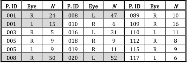
An ophthalmologist segmented manually a sub-database of eighteen series, for the quantitative evaluation of the proposed
processing methods (Table 1). These series feature
different characteristics in terms of disease progress, lesion shape, size, image quality. For 3 patients, we have series for both left and right eyes. The number of images per series ranges from 5 to 52 (18.2±15.9 in average), with a total of 328 segmented images. We have images at the very beginning of the disease for 5 series. In this case, there is no apparent GA in the first image(s).
P. ID Eye N P. ID Eye N P. ID Eye N
001 R 24 008 L 47 089 R 10 001 L 15 010 R 6 109 R 16 003 R 5 016 L 31 110 L 11 005 R 9 018 R 9 112 R 8 005 L 9 019 R 11 115 R 9 008 R 50 020 L 52 117 L 6
Table 1.Sub-database used in the quantitative evaluation Patient ID, processed eye, left (L) or right (R), number of images in the series (N). Background in light gray when the acquisitions start with no GA (5 series).
We developed several user-guided segmentation tools to make the ground truth, based on classical segmentation algorithms: thresholding applied locally on a rectangle defined by the user, parametric active contour model initialized by the user, simple linear interpolation between points entered by the user. The user chooses the most appropriate tool to locally delimit the lesion border, and thus progresses step by step. Automatic thresholding or active contour algorithm initialized by the user leads to segmentations that depend less on the user than the only use of interpolation, and the expert was encouraged to apply these tools as often as possible. However, the segmentation remains mostly manual, user-dependent and tedious. An ophthalmologist realized all segmentations used in our experiments. This has been a very hard and long task: as previously mentioned, GA boundaries may be very indented; moreover, there is very often a strong ambiguity on the true position of the GA border and on the appearance or not of new injured areas. Consequently, the expert had often to go through the images to make or review a decision. On average, it took 10 minutes to process one single image.
4. Methods
Let us denote by 𝑋𝑛, 𝑛 ∈ [1, 𝑁] the series of acquired images,
to be processed. The grayscale pixels are coded by floating point numbers in the interval [0,1]. Our method is made of two main steps: an image normalization to compensate for illumination variation between images, and morphological processing to enhance the consistent changes between images and attenuate artefacts.
4.1. Normalization step
We consider the model where each acquired image 𝑋𝑛, 𝑛 ∈
[1, 𝑁], is the pixel-wise product of an image of reflectance 𝑅𝑛 and
an image of illumination 𝐼𝑛:
𝑋𝑛= 𝑅𝑛𝐼𝑛, 𝑛 ∈ [1, 𝑁] (1)
Our goal is to compensate for illumination variation (i.e. the fact that 𝐼𝑛 ≠ 𝐼𝑚 for 𝑛 ≠ 𝑚) to get homogeneous illumination
between all processed images. In other words, we aim at calculating from 𝑋𝑛 a new series of images, 𝑌𝑛= 𝑅𝑛𝐽𝑛, where 𝐽𝑛
is the corrected illumination of the nth image, with 𝐽
𝑛= 𝐽𝑚 for all
pairs. Note that the illumination can remain uneven over the image domain, but this inhomogeneity must be the same in all images of the series to allow differential analysis.
4
The illumination variation is generally smooth, and we canassume that the pixel-wise ratios 𝐼𝑛+1⁄ only contain low 𝐼𝑛 frequencies. As there are only few and only small structural changes between two consecutive images, we can also consider that the lowpass filtered version of the ratio 𝑋𝑛+1⁄𝑋𝑛 is a good
estimate of 𝐼𝑛+1⁄ . So we calculate 𝐼𝑛 𝑈𝑛= ( 𝐼𝑛+1 𝐼𝑛 ) ̂ =𝑋𝑛+1 𝑋𝑛 ∗ 𝑓𝜎, 𝑛 ∈ [1, 𝑁 − 1] (2)
where 𝑓𝜎 is a Gaussian kernel with standard deviation 𝜎 and * the
convolution operator. 𝜎 is a scale parameter, chosen to remove structural change areas between consecutive images. Then we estimate the ratio of illumination for any pair of images in a recursive way: ∀(𝑛, 𝑚) ∈ [1, 𝑁]2, 𝑚 ≥ 𝑛, (3) 𝑉𝑚,𝑛= ( 𝐼𝑚 𝐼𝑛) ̂ = 𝑈𝑚−1𝑉𝑚−1,𝑛 𝑉𝑛,𝑚= 1 𝑉𝑚,𝑛
So, the lowpass filter 𝑓𝜎 is only applied on ratios of consecutive images, so with little change from one to the other, and not on any other pairs where the reflectance is likely to be very different, with large areas of change. Our goal is to apply an algorithm that corrects the images, so that the new illumination ratio becomes close to 1 at each pixel, and that for any pair (𝑚, 𝑛). To achieve that, our preliminary idea was to propose an iterative algorithm that modifies each image against the (𝑁 − 1) others:
∀(𝑚, 𝑛), 𝑚 > 𝑛, { 𝑌𝑛 (𝑖+1) = 𝑌𝑛(𝑖)𝑉𝑚,𝑛(𝑖) 𝛼 2 𝑌𝑚(𝑖+1)= 𝑌𝑚(𝑖)𝑉𝑚,𝑛(𝑖) − 𝛼 2 (4)
where 𝑖 denotes the iteration, 𝑌𝑛(0)= 𝑋𝑛, 𝑉𝑚,𝑛(𝑖) is the updated
estimate of the illumination ratio.
Let us assume that the illumination at a given pixel (𝑥, 𝑦) is higher in 𝑌𝑚(𝑖) than in 𝑌𝑛(𝑖). Then its illumination in the nth image
will be multiply by a factor 𝑉𝑚,𝑛(𝑖) 𝛼
2(𝑥, 𝑦) > 1 while its illumination in
the mth image will be divided by the same factor, resulting that the
new illumination values in 𝑌𝑛(𝑖+1) and 𝑌𝑚(𝑖+1) become closer. Processing all pairs in this way enables us to correct every image against all the others. The parameter 𝛼 controls the amount of correction brought by each image of the series to process another one. Thus, we can assume that the illumination distortion between images progressively decreases so that, after 𝐿 iterations, we get a new series 𝑌𝑛= 𝑌𝑛(𝐿) with same illumination in all images: 𝐼𝑚(𝐿)=
𝐼𝑛(𝐿) for all pairs (𝑛, 𝑚). Note that the algorithm in equation (4) is equivalent to ∀𝑛, 𝑌𝑛(𝑖+1)= 𝑌𝑛(𝑖)∏ 𝑉𝑘,𝑛(𝑖) 𝛼 2 𝑁 𝑘=1 (5)
Let us now go farther in the interpretation by studying the convergence of the proposed algorithm. For that, we consider the particular case where all images have the same reflectance but were acquired under different illuminations. For any pair, we have 𝑉𝑘,𝑛(𝑖)= 𝐼𝑘(𝑖)⁄𝐼𝑛(𝑖)= 𝑌𝑘(𝑖)⁄𝑌𝑛(𝑖) and the correction algorithm becomes
∀𝑛, 𝑌𝑛(𝑖+1)= 𝑌𝑛(𝑖)∏ ( 𝑌𝑘(𝑖) 𝑌𝑛(𝑖) ) 𝛼 2 𝑁 𝑘=1
We denote by 𝑍𝑛(𝑖) the logarithm of 𝑌𝑛(𝑖). We have ∀𝑛, 𝑍𝑛(𝑖+1)= 𝑍𝑛(𝑖)+𝛼 2∑ (𝑍𝑘 (𝑖) − 𝑍𝑛(𝑖)) 𝑁 𝑘=1 (6)
At iteration 𝑖, we define the difference between any two images: Δ𝑛,𝑚(𝑖) = 𝑍𝑛(𝑖)− 𝑍𝑚(𝑖)
At the next iteration, we have Δ𝑛,𝑚(𝑖+1)= 𝑍𝑛(𝑖+1)− 𝑍𝑚(𝑖+1)= (1 −𝛼𝑁 2) Δ𝑛,𝑚 (𝑖) For 0 < 𝛼 <2 𝑁 we have 𝑖→∞limΔ𝑛,𝑚 (𝑖)
= 0 for any pair of images, meaning that the algorithm converges to a common image. From equation (6) we notice that the mean value of all images is constant and equal to 1
𝑁∑ log 𝑋𝑛 𝑁
𝑛=1 . Consequently the final corrected
image, after convergence, is the geometric average of all input images: ∀𝑛, lim 𝑖⟶∞𝑌𝑛 (𝑖) = (∏𝑁 𝑋𝑘 𝑘=1 ) 1 𝑁
Thus, our final corrected images, all equal to the geometric average of the input images, are given by
𝑌𝑛 = 𝑋𝑛𝐹𝑛 with 𝐹𝑛=(∏ 𝑋𝑘 𝑁 𝑘=1 ) 1 𝑁 𝑋𝑛 = ∏ (𝐼𝑘 𝐼𝑛) 1 𝑁 𝑁 𝑘=1 (7)
As we are not in this ideal case where all images have the same reflectance, our strategy will be to estimate all illumination ratios as described by equations (2) and (3), and to calculate in just one pass the corrected images:
𝑌𝑛 = 𝑋𝑛𝐹𝑛 with 𝐹𝑛= ∏ 𝑉𝑘,𝑛
1 𝑁
𝑁
𝑘=1 (8)
Finally, our correction algorithm is as follows: Input : series of images 𝑋𝑛, 𝑛𝜖[1, 𝑁]
• Calculate 𝑈𝑛 for 𝑛𝜖[1, 𝑁 − 1] (2)
• Calculate 𝑉𝑘,𝑛 for all pairs (𝑘, 𝑛) (3)
• Calculate new images 𝑌𝑛 (8)
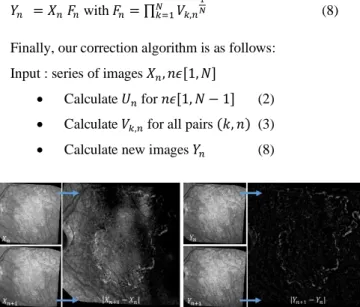
Fig. 2. Joint normalization applied on series 005-L. On the left, two consecutive source images 𝑋𝑛.and 𝑋𝑛+1 and their difference |𝑋𝑛+1− 𝑋𝑛|. On
the right, the same after normalization.
The low-pass filtering in equations (2) and (3) gives only an approximation of the illumination ratio between two images. Therefore, considering all pairs (𝑚, 𝑛) of images, even when the two medical exams were done at a large time interval, with important reflectance changes, is probably not appropriate, even with our recursive approach. For that reason, we propose to implement the algorithm with a sliding temporal window: each image is corrected considering 2𝐾 + 1 images, 𝐾 images acquired
5
before and 𝐾 images acquired after the processed image. Theoverlap ensures that all images of the series will converge to the same illumination. Experiments showed that2 ≤ 𝐾 ≤ 7 (5 to 15 images in the window) are good values for our dataset (Section 5.2). Fig. 2 shows an example of two consecutive images extracted from a series of 9 images. We observe that the initial absolute difference does not provide meaningful information, while it reveals the GA growth after normalization.
The proposed algorithm corrects each image with respect to all the others. However, the new illumination generally remains spatially uneven. It is certainly possible to compensate for this distortion when the series begins without any GA, thanks to classical background subtraction technics. This has not been explored yet.
4.2. Enhancement step
The second step of our algorithm exploits prior knowledge about the studied disease: we know that the GA, which is brighter than the surrounding structures, growths continuously, without any chance of recovery. It means that the GA in image 𝑌𝑛 is included in the GA in 𝑌𝑚>𝑛. Therefore, we apply morphological reconstructions to all triplets 𝑌𝑛−1, 𝑌𝑛,, 𝑌𝑛+1 as follows:
𝑍𝑛 = (𝑌𝑛 𝑅𝐷𝑌𝑛 (𝑌 𝑛−1) 𝑅𝐸 𝑌𝑛 (𝑌 𝑛+1)) 1 3 (9) where 𝑅𝐷𝑀 (𝑆) (resp. 𝑅𝐸𝑀 (𝑆)) denotes the reconstruction by
dilation (resp. erosion) of the marker S in the mask M. The first reconstruction ensures that we keep only bright areas that were already present in the previous image. The second one suppresses bright areas that are not present in the next image. The pixel-wise product to the power 1/3 merges all these conditions and enhances the meaningful bright areas in image 𝑛. The normalizing algorithm is applied again on the images 𝑍𝑛,, to ensure that the new series is
properly normalized and to further reduce the influence of artefacts.
(a) (b)
(d) (c)
Fig. 3. Normalization and image enhancement. (a) Three consecutive images 𝑋𝑛−1, 𝑋𝑛, 𝑋𝑛+1, 𝑛 = 30; the corresponding normalized images before
(b) and after (c) morphological processing. The green arrows point to a part of the actual GA and the red arrows to bright artefacts; (d) corresponding difference images, emphasized by a factor 3, before normalization (left), after normalization (middle), after normalization and morphological processing (right). The normalization reveals the GA growth but light artefacts are also enhanced (inside the red circle); the morphological processing reduces the intensity of artefacts (green circle).
Fig. 3 shows an example of the whole processing on 3 consecutive images. The difference image is calculated by 𝑚𝑎𝑥{|𝑋𝑛+1−𝑋𝑛|, |𝑋𝑛−𝑋𝑛−1|}. The first step (normalization)
enables us to enhance the differences between the images, while
the second step (morphological processing) attenuates the bright artefacts that are not new lesions.
5. Results
We rely on the manual segmentations performed by our expert (18 series, 328 images in total) to evaluate the proposed methods, in two different ways: though the estimation of the contrast between the GA and the background (i.e. surrounding tissues and anatomical structures) and through the evaluation of preliminary segmentation results based on automatic thresholding.
5.1. Ground truth
Let us denote by 𝐺𝑇𝑛 the binary image of the GA segmentation made by the medical expert in the nth image of a series. The inside
of the GA delineated by the expert is set to 1 and the outside to 0. To deal with possible errors and inconsistencies (such as 𝐺𝑇𝑛⊄
𝐺𝑇𝑚>𝑛), we estimate the inside 𝐿𝑛(𝑖𝑛) of the GA in image 𝑛 and the outside 𝐿𝑛(𝑜𝑢𝑡) by:
𝐿(𝑖𝑛)𝑛 = ⋃𝑛𝑘=1𝐺𝑇𝑘
𝐿(𝑜𝑢𝑡)𝑛 = 𝐿̅̅̅̅̅̅ (𝑖𝑛)𝑛 (10) where 𝐸̅ denotes the complement of the set 𝐸. This choice ensures that 𝐿(𝑖𝑛)𝑛 ⊆ 𝐿(𝑖𝑛)𝑛+1.
To deal with series where a GA is already present in the first image (13 series over 18), we define the total growth of the GA from the first image to the nth by:
𝐺𝑇ℎ𝑛= 𝐿𝑛(𝑖𝑛)∩ ⋂̅̅̅̅̅̅̅̅̅̅̅̅ 𝑁𝑘=1𝐺𝑇𝑘 (11)
Finally, the growth between two images is given by 𝑔𝑡ℎ𝑛:𝑚>𝑛= 𝐺𝑇ℎ𝑚∩ 𝐺𝑇ℎ̅̅̅̅̅̅̅ 𝑛 (12) These three equations gives us the ground truth for the GA segmentation (10), the growth from the first image to the nth (11)
and the growth between two images (12). We rely on these definitions to evaluate our methods.
We also estimate the contrast between two regions, denoted by 𝑅1 and 𝑅2, in a given image 𝑋, by calculating the mean signal power 𝑃(𝑋, 𝑅) in these two regions, and then the difference ∆𝑃(𝑋, 𝑅1, 𝑅2) in dB: 𝑃(𝑋, 𝑅) = 10 log10[ 1 |𝑅|∑ (𝑋(𝑥, 𝑦)) 2 (𝑥,𝑦)∈R ] (13)
where |𝑅| denotes the number of pixels in the region 𝑅. ∆𝑃(𝑋, 𝑅1, 𝑅2) = 𝑃(𝑋, 𝑅1) − 𝑃(𝑋, 𝑅2) (14)
The higher |∆𝑃(𝑋, 𝑅1, 𝑅2)|, the higher the mean contrast in 𝑋 between the two regions 𝑅1 and 𝑅2 and the easier the two regions
can be segmented. This measure will help us to evaluate the benefit of our algorithms by comparing the contrast between healthy and unhealthy areas in images derived from 𝑋𝑛 (source images), 𝑌𝑛
(after normalization) and 𝑍𝑛 (after morphological processing).
5.2. Evaluation from variance images calculated along the temporal axis
Our algorithm aims at correcting illumination variations between images. As a result, the illumination may be still uneven in every image, but it should be the same in all images of the series. So, the gray level of a pixel belonging to an healthy region (outside
6
the GA in all images) must be stable in the series (low variance),contrary to a pixel belonging to a region of GA growth whose gray level increases significantly at a given time. Consequently, we can evaluate the benefit of our normalization algorithm by estimating the contrast between these two regions in a variance image.
We consider a sliding temporal window of 𝑀 = 2𝑚 + 1 consecutive images (Fig. 4). For each image 𝑛 ∈ [𝑚 + 1, 𝑁 − 𝑚] we take the images 𝑋𝑛−𝑚 to 𝑋𝑛+𝑚 to calculate the variance of the gray levels at each pixel. We denote by 𝑋𝑛(𝑉𝐴𝑅) the resulting image. We consider the heathy region 𝑅𝑛(ℎ𝑒𝑎𝑙𝑡ℎ𝑦)= 𝐿𝑛+𝑚(𝑜𝑢𝑡) and the region of growth 𝑅𝑛(𝑔𝑟𝑜𝑤𝑡ℎ)= 𝑔𝑡ℎ𝑛−𝑚:𝑛+𝑚, and we evaluate the contrast
between both: ∆𝑃(𝑋𝑛 (𝑉𝐴𝑅)
, 𝑅𝑛(𝑔𝑟𝑜𝑤𝑡ℎ), 𝑅𝑛(ℎ𝑒𝑎𝑙𝑡ℎ𝑦)) (13)(14). We average the results in the series and over all series to get mean values, denoted by ∆𝑃(𝑋𝑉𝐴𝑅).
Fig. 4. Variance images calculated over 𝑀 = 2𝑚 + 1 consecutive images. Mean power values are interpreted by considering the GA growth over this temporal window (𝑅𝑛(𝑔𝑟𝑜𝑤𝑡ℎ)) and the still healthy area (𝑅𝑛(ℎ𝑒𝑎𝑙𝑡ℎ𝑦)).
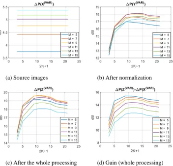
(a) Source images (b) After normalization
(c) After the whole processing (d) Gain (whole processing) Fig. 5. Contrast enhancement between the GA growth area and the healthy area for several parameters 𝐾 (temporal window in the normalization algorithm) and 𝑀 (temporal window to compute the variance).
Fig. 5 displays the results for different sizes of sliding window in the normalization algorithm (2𝐾 + 1, Section 4.1), different sizes of sliding window to compute the variance images (𝑀 = 2𝑚 + 1 ∈ {5,9,11,13,15}), and at different steps of the algorithm: on the source images (𝑋𝑛), after normalization (𝑌𝑛) and
after morphological processing (𝑍𝑛). We consider only the 6 series
having more than 15 images (maximum value for 𝑀) with GA, for the sake of comparison. These results demonstrate the benefits of our algorithm with great improvements of the contrast whatever the parameter 𝐾 and the length of the analysis (M): the gain ranges from 11 to 15dB (Fig. 5d) after the whole processing. Most of the gain results from the normalization algorithm but the
morphological processing contributes also to enhance the
GA growth area (about +1.5dB). Setting 2𝐾 + 1 = 11 leads to the highest contrasts (b,c) whatever 𝑀. But this experiment shows also that 𝐾 is not a sensitive parameter since the performances remain similar for (2𝐾 + 1) ∈ [5,21].
5.3. Evaluation from an enhanced image of the GA total growth
Let us define the image 𝐺𝑛(𝑋)enhancing the area of growth
between the first and the nth image:
𝐺𝑛(𝑋)= max
𝑘∈[2,𝑛],𝑙<𝑘(𝑋𝑘− 𝑋𝑙), 𝑛 ∈ [2, 𝑁] (15)
Note that maximizing over all differences, (𝑋𝑘− 𝑋𝑙) with 𝑙 < 𝑘, makes sense only because all images have been jointly normalized. We compare the signal power in the total growth area 𝐺𝑇ℎ𝑁 (11) to the power outside the GA, 𝐿(𝑜𝑢𝑡)𝑁 (10), by calculating ∆𝑃(𝐺𝑁
(𝑋)
, 𝐺𝑇ℎ𝑁, 𝐿𝑁 (𝑜𝑢𝑡)
) (13)(14) at the different steps of the algorithm. Table 2 summarizes the results averaged on the 18 series of the experimentation sub-database. The main gain obviously results from the normalization step, but the morphological treatment improves generally slightly the contrast, (+0.5dB). The results are again stable over 𝐾, with slightly better contrasts for 2𝐾 + 1 = 9. ∆𝑷(𝑮𝑵(𝑿)) 𝑲 ∆𝑷(𝑮𝑵(𝒀)) Gain ∆𝑷(𝑮𝑵(𝒁)) Gain 2.76 ± 3.47 2 8.44 ± 2.42 5.68 ± 2.44 9.52 ± 2.10 6.76 ± 3.03 4 𝟗. 𝟐𝟓 ± 𝟐. 𝟏𝟑 𝟔. 𝟒𝟗 ± 𝟑. 𝟔𝟕 𝟗. 𝟕𝟎 ± 𝟏. 𝟕𝟔 𝟔. 𝟗𝟑 ± 𝟑. 𝟔𝟐 5 9.06 ± 2.06 6.30 ± 3; 79 9.52 ± 1.81 6.75 ± 3.50 6 8.95 ± 2.08 6.19 ± 3; 70 9.49 ± 1.91 6.73 ± 3.36 Table 2. Contrast between the area of GA growth 𝐺𝑇ℎ𝑁 and the outside
𝐿𝑁 (𝑜𝑢𝑡)
in the enhanced image (15) calculated from 𝑋𝑛, 𝑌𝑛 or 𝑍𝑛. The gains are
calculated with respect to the initial contrast ∆𝑃(𝐺𝑁
(𝑋)). Values are in dB 𝑋1 𝑋𝑁, 𝑁 = 24 𝐺𝑁 (𝑋) 𝐺𝑁 (𝑋,𝑆𝐸𝐺) 𝑍1 𝑍𝑁, 𝑁 = 24 𝐺𝑁 (𝑍) 𝐺 𝑁 (𝑍,𝑆𝐸𝐺)
Fig. 6. GA growth enhancement and segmentation, applied on a series of 24 images with no lesion in the first image (Patient 001-R). The first row shows the images before normalization (𝑋𝑛) and the second row after
processing (𝑍𝑛). The enhanced GA growth is shown in the third column and
the corresponding segmentation in the fourth column (F1 score: 0.77 for 𝐺𝑁(𝑍,𝑆𝐸𝐺)).
Fig. 6 shows the enhanced GA growth (15) before and after processing. In this example, the set of images starts from the very early stages of the disease to advanced ones and the whole GA is enhanced with a very dark background (𝐺𝑁
(𝑍)) compared to the
result without processing (𝐺𝑁
(𝑋)). The growth of diseased tissues
around the optical disk is also clearly visible.
A simple thresholding with Otsu’s method enables us to segment the total GA growth, thanks to the proposed processing, while it was impossible with the source images (Fig. 6). We denote by 𝐺𝑁(𝑋,𝑆𝐸𝐺) the binarized 𝐺𝑁(𝑋) image. The segmentation is evaluated in Table 3 via classical metrics: precision, recall and
F1-7
score, which is the harmonic mean of precision and recall, giventhe ground truth 𝐺𝑡ℎ𝑁 (11).
Lesion (5 series) Growth (13 series)
𝑇𝑂𝑡𝑠𝑢 Prec. Rec. F1-sc. Prec. Rec. F1-sc.
𝐺𝑁(𝑋,𝑆𝐸𝐺) 0.44 0,29 0,86 0,42 0,27 0,63 0,33 ±0.04 ±0,10 ±0,15 ±0,13 ±0,23 ±0,16 ±0,17 𝐺𝑁(𝑌,𝑆𝐸𝐺) 0.33 0,82 0,75 0,77 0,50 0,68 0,53 ±0.02 ±0,15 ±0,15 ±0,10 ±0,27 ±0,12 ±0,20 𝐺𝑁(𝑍,𝑆𝐸𝐺) 0,37 0,86 0,76 0,80 0,52 0,65 0,53 ±0,02 ±0,09 ±0,14 ±0,09 ±0,26 ±0,12 ±0,18 Table 3. Evaluation of the GA growth segmentation by Otsu’s method at the different steps of the algorithm.
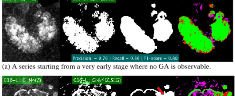
(a) A series starting from a very early stage where no GA is observable.
(b) A series starting from an advanced stage. Texture changes inside the lesion are classified as lesion growth areas ( ), resulting in low precision. The recall is low since the expert segmented the right part as lesion in the last image ( ), contrary to the algorithm.
Fig. 7. Segmentation of the GA growth. Left to right: enhanced image 𝐺𝑁(Z), proposed segmentation 𝐺𝑁(Z,SEG), ground truth 𝐺𝑡ℎ𝑁, and comparison
(true positives in green, false negatives in red and false positives in magenta).
The best scores are achieved with the whole processing, normalization and morphological treatment. We notice that Otsu’s threshold (𝑇𝑂𝑡𝑠𝑢) is remarkably stable over the series (0.37 ±
0.02). The results for the detection of the whole growth are especially good with a F1-score equal to 0.80±0.09 (Table 3, Fig. 6a). For the other series, the F1-score is much lower, equal to 0.53±0.18. The main problem is that the texture changes inside the GA over time, resulting in a lot of false positives and lower precision (Fig. 6b).
5.4. GA progress between consecutive images
Finally, still with the aim of evaluating our image processing algorithms, we tried to segment the GA growth between consecutive images. This process is a prerequisite to elaborate predictive models of the disease. For that, we consider the pixels belonging to the GA growth area, so satisfying 𝐺𝑁(𝑍,𝑆𝐸𝐺)(𝑥, 𝑦) = 1
(Section 5.3), and we study their gray levels in the whole series. Let us denote by 𝑉(𝑍,(𝑥,𝑦))(𝑛), 𝑛 ∈ [1, 𝑁], the gray levels of such a
pixel (𝑥, 𝑦) in the processed series 𝑍𝑛. We assume that this pixel is not part of the GA in the first image and that it will be included in the GA at a given time 𝑡. This means that the gray levels in
𝑉(𝑍,(𝑥,𝑦)) may be low for 1 ≤ 𝑛 < 𝑡 and much higher for 𝑡 ≤ 𝑛 ≤
𝑁 and roughly stable in the two states. For each index 𝑘 ∈ [2, 𝑁], we classify the elements of 𝑉(𝑍,(𝑥,𝑦)) in 2 classes: 𝑉(𝑍,(𝑥,𝑦))(𝑛) ∈
𝐶0(𝑘) if 𝑛 < 𝑘, 𝑉(𝑍,(𝑥,𝑦))(𝑛) ∈ 𝐶1(𝑘) otherwise. We calculate the
inter-class variance according to Otsu’s criterion for each index 𝑘:
𝜎𝑂𝑡𝑠𝑢2 (Z,(𝑥,𝑦)) (𝑘) =𝑘 − 1 𝑁 (𝑉1:𝑘−1 (𝑍,(𝑥,𝑦)) ̅̅̅̅̅̅̅̅̅̅̅ − 𝑉̅̅̅̅̅̅̅̅̅̅̅1:𝑁(𝑍,(𝑥,𝑦))) 2 + 𝑁−𝑘+1 𝑁 (𝑉𝑘:𝑁 (𝑍,(𝑥,𝑦)) ̅̅̅̅̅̅̅̅̅̅̅ − 𝑉̅̅̅̅̅̅̅̅̅̅̅1:𝑁(𝑍,(𝑥,𝑦)))2 (16)
where 𝑉̅̅̅̅̅̅̅̅̅̅̅𝑘:𝑙(𝑍,(𝑥,𝑦)) denotes the mean value of the elements k to l of vector 𝑉(𝑍,(𝑥,𝑦)). We calculate a segmentation map by maximizing
the interclass variance 𝜎𝑂𝑡𝑠𝑢2 (Z,(𝑥,𝑦)) : 𝑀𝐴𝑃(𝑍)(𝑥, 𝑦) = arg max
𝑘 𝜎𝑂𝑡𝑠𝑢 2 (Z,(𝑥,𝑦))
(𝑘) (17) This method is not relevant for pixels that do not switch from an heathy to an unhealthy state. Consequently the method is only applied in the GA growth area, so for pixels satisfying
𝐺𝑁(𝑍,𝑆𝐸𝐺)(𝑥, 𝑦) = 1 (Section 5.3). So we calculate the series
𝑆𝐸𝐺𝑛(𝑍), 𝑛 ∈ [1, 𝑁], of binary images of the GA from image 1 to image 𝑁 by
𝑆𝐸𝐺𝑛(𝑍)(𝑥, 𝑦) =
{1 if 𝑛 ≥ 𝑀𝐴𝑃(𝑍)(𝑥, 𝑦) and 𝐺𝑁
(𝑍,𝑆𝐸𝐺)(𝑥, 𝑦) = 1
𝑂 otherwise (18)
Finally we calculate the growth between two consecutive images by
𝑆𝐸𝐺𝑛−1:𝑛(𝑍) = 𝑆𝐸𝐺𝑛(𝑍) & 𝑆𝐸𝐺̅̅̅̅̅̅̅̅̅̅𝑛−1(𝑍) (19) which reveals the progression of the GA between the (𝑛 − 1)th and
the 𝑛th images.
Table 4 shows the quantitative evaluation of this segmentation method, applied on the processed series 𝑌𝑛 and 𝑍𝑛. The method is
obviously not applicable before normalization. The automatic segmentation 𝑆𝐸𝐺𝑛−1:𝑛(𝑌,𝑍) is compared to the manual segmentation
𝑔𝑡ℎ𝑛−1:𝑛 (12) using the classical metrics, which are averaged over the images n and then over the series. Fig. 8 shows samples of growth segmentation between consecutive images (𝑆𝐸𝐺𝑛−1:𝑛(𝑍) , (19)) in one series, and Fig. 9 colored representations of the GA growth (𝑀𝐴𝑃(𝑍), (17)) for two different series, along with the corresponding ground truth.
Lesion (5 series) Growth (13 series)
Prec. Rec. F1-sc. Prec. Rec. F1-sc. 𝑆𝐸𝐺𝑛−1:𝑛 (𝑌) 2𝐾 + 1 = 9 0.21 0.23 0.19 0.20 0.28 0.21 ±0.12 ±0.13 ±0.11 ±0.12 ±0.12 ±0.11 𝑆𝐸𝐺𝑛−1:𝑛(𝑍) 2𝐾 + 1 = 5 0.25 0.24 0.19 0.23 0.31 0.24 ±0.12 ±0.12 ±0.10 ±0.13 ±0.14 ±0.12 Table 4. Evaluation of the segmentation of the GA progress between consecutive images. The results are given for the series 𝑌𝑛 and 𝑍𝑛 with the
optimal value of 𝐾 in both cases.
Overall, the segmentation images 𝑆𝐸𝐺𝑛−1:𝑛(𝑍) (Fig. 8) look very consistent, and the colored maps (Fig. 9) look similar to their equivalent deduced from the ground truth. However the average metrics are quite low (Table 4). There are several explanations for this. First, it should be remembered that the manual segmentation is very difficult to achieve and is not accurate either. Second, the GA progress between two consecutive images is structurally very thin, which explains that a small difference between the segmented area and the ground truth results immediately in low metrics.
8
Especially, small shifts in the change detection maps lead to anincrease of false positives and false negatives, therefore to weaker metrics, although the automatic GA growth detection is not bad (Fig. 8).
Fig. 8. Examples of very consistent change detections between consecutive images, with F1 scores. Every time, the automatic segmentation 𝑆𝐸𝐺𝑛−1:𝑛(𝑍) (19) is on the left and the ground truth 𝑔𝑡ℎ𝑛−1:𝑛 (12) on the right.
Fig. 9. Colored map of the GA progress in the series (17). The nth color in the
colormap corresponds to a GA progress between image n-1 and image n. The automatic result is on the left and the ground truth on the right. The F1 score is the average of all F1 scores obtained for each pair of consecutive images (19).
(a) (b)
Fig. 10. Limits of the segmentation method. In each illustration, the automatic result is on the left and the ground truth on the right. (a) Case of a series of 9 images corresponding to late stages of ARMD. The area of total GA growth 𝐺𝑁(𝑍,𝑆𝐸𝐺) is over segmented (first row) leading to many false positives in the detection of changes between consecutive images, inside and outside the GA (second row). (b) Case of a series starting from the beginning of the disease. Texture changes over time result in false positives inside the GA, and the F1 score is low despite the good detection of the border growth (top). This results also in differences in the colored maps 𝑀𝐴𝑃(𝑍) (bottom).
Finally, the main limits of the proposed segmentation method come from the texture changes inside the lesion during the growth, disturbing the decision criterion (high variance in the class 𝐶1). In
addition, an over-segmentation of the total growth (𝐺𝑁 (𝑍,𝑆𝐸𝐺)
) allows false positives inside and outside the GA (18), and this has a strong impact on the precision and on the F1 score, especially for series
starting with advanced GA for which we have a low
precision in the 𝐺𝑁(𝑍,𝑆𝐸𝐺) segmentations (0.52 ± 0.26, Table 3). Fig. 10 illustrates these problems. All this explains the rather low metrics presented in Table 4, despite consistent detections of changes. The best results are obtained on average with the normalized images processed by mathematical morphology (𝑍𝑛),
for 𝐾 = 5, with a F1 score around 0.21 ± 0.12. For the normalized series 𝑌𝑛, the best scores are for 𝐾 = 9, and are slightly lower than those for the images 𝑍𝑛. The morphological treatment improves
the results by introducing a better consistency along the temporal axis.
However, these first results are already interesting, given that the segmentation method is basic, without any spatial regularization. Despite all previously mentioned problems, the normalization algorithm and the morphological processing make it possible to produce interpretable colored maps, and better results are likely to be obtained with more advanced segmentation algorithms.
6. Discussion
We have presented a set of experiments evaluating the advantages of our normalization algorithm for the direct comparison of gray levels in a series of fundus images, and, ultimately, the detection of the GA growth by differential analysis. We first calculated the variance at each pixel, which must be low in the areas that remain healthy and, if applicable, within the GA present in the first image, and high in the region of GA growth (Section 5.2). We found that our processing increases the contrast between the growth area and the rest of the image by 11 to 15dB (Fig. 5), which is very important. It means that the visual inspection of the series, by scrolling through the images, is greatly facilitated, since illumination distortions no longer disturb the interpretation. The GA expansion becomes much more visible. The main gain results from the illumination normalization, but the morphological treatment attenuates local artefacts that could be mistaken for new GA zones. This experiment demonstrates also the advantage of normalizing on a sliding window and helps us to set its optimal size (around 11 consecutive images).
In addition, the proposed preprocessing enables us to perform a differential analysis, in order to detect the GA growth between any two examinations. Thus, in Section 5.3, we calculated an enhanced image of the total GA growth and we demonstrated that the contrast between the GA growth area and the outside (still heathy region) is around 10dB while it was only around 3dB without treatment (Table 2). The gain enables a segmentation of the GA growth area with a F1-score equal to 0.80 ± 0.09 for series starting from the earliest stages of the disease, while it was only equal to 0.42 ± 0.13 without treatment (Table 3). The segmentation methods is basic, based on Otsu’s thresholding, but the results are already good despite this. The segmentation of the GA growth from an already advanced stage is less good, with an average F1-score equal to 0.53 ± 0.18 (0.33 ± 0.17 without treatment). This is due to texture changes inside the lesion during time, resulting in higher values in the difference images, and therefore lower precision. Finally, we explored the possibility of calculating colored maps of the GA progress, in order to obtain a visualization of the growth and speed of growth in a single image (Section 5.4). The proposed method is based on the idea that the grey-levels are stable in each state, healthy (low values) or unhealthy (high value). We faced again the problem of texture variations inside the GA that disturb the detection of the time at which a pixel has switched from a healthy state to an unhealthy one. However, we got nice maps in some cases (Fig. 9), close to the ground truth, and also very good sets of binary images showing
9
the GA growth between two consecutive images. The F1-scoresevaluating the segmentation of the GA growth between consecutive images are not high (around 0.21 ± 0.12 on the whole database), but these poor results should be put into perspective, as the structures to be detected are very thin and the manual segmentation prone to inaccuracies. We measured weak metrics in many cases despite the binary images of change looked very consistent (Fig. 8).
All these experiments demonstrate that the proposed processing enables the detection of changes between any two images of a series of fundus images, regardless the number of images, the size and shape of the GA. This is very new compared to the literature, which has focused much more on the segmentation of the GA in single images (Section 2), and much less on change detection in series [10][13]. Contrary to [10], we normalize all images jointly and not just in pairs, and the differential analysis proposed in [13], where the images are preprocessed separately by a homomorphic filter, could benefit from our global normalization.
7. Conclusion and perspectives
Very large databases of patients available through routine imaging systems offer an opportunity to study a vast amount of data on dry ARMD. Especially, deriving models of GA progression from fundus images is of high medical interest, in order to better understand the intimate mechanisms of lesion growth or to assess the benefit of treatments. However, there is a real lack of automatic algorithms to process all these images, and especially to detect and quantify the GA progression between two medical examinations. Many research works deal with the GA segmentation in single images, but there is not yet an automatic and reliable solution. A promising alternative is to carry out a differential analysis between consecutive images, but the first obstacle is the great illumination inhomogeneity inside the images and especially between the images. This article deals with the correction of illumination inhomogeneity between all the images in a series in order to allow the differential analysis between any two images. For that, we have proposed a method which recursively estimates the illumination ratio between any two images in the series and correct the illumination of every image to the geometric mean of all illuminations. Then, we have presented a morphological processing that enhances the consistent changes between consecutive images and attenuate the others, based on the fact that the GA increases continuously. Finally, we have presented many experiments realized on a database of 18 series (328 images) acquired from 15 patients and segmented manually by a medical expert. The experiments show the benefit of the normalization algorithm and of the morphological processing, in terms of contrast between the healthy area and the GA growth area, and in terms of ability to detect cumulative changes in the series or between consecutive images. The experimental results demonstrate that the normalization algorithm makes possible the differential analysis, and that the morphological processing brings some improvements by attenuating light artefacts. Our first attempt to detect the GA growth in consecutive images shows that it is possible to process all the images of the series jointly, since the gray levels are now comparable at each pixel. We got very nice colored maps of GA progression, offering an intuitive understanding for clinicians, in terms of growth and speed of growth. However, a more robust segmentation algorithm, integrating spatial and temporal regularization, is required to obtain more reliable and more accurate maps of the GA growth.
8. References
[1] Deckert, A., Schmitz-Valckenberg, S., Jorzik, J., Bindewald, A., Holz, F. G., & Mansmann, U. (2005). Automated analysis of digital fundus
autofluorescence images of geographic atrophy in advanced age-related macular degeneration using confocal scanning laser ophthalmoscopy (cSLO). BMC ophthalmology, 5(1), 8.
[2] Feeny, A. K., Tadarati, M., Freund, D. E., Bressler, N. M., & Burlina, P. (2015). Automated segmentation of geographic atrophy of the retinal epithelium via random forests in AREDS color fundus images. Computers in biology and medicine, 65, 124-136.
[3] Hu, Z., Medioni, G. G., Hernandez, M., Hariri, A., Wu, X., & Sadda, S. R. (2013). Segmentation of the geographic atrophy in spectral-domain optical coherence tomography and fundus autofluorescence images. Investigative ophthalmology & visual science, 54(13), 8375-8383.
[4] Hu, Z., Medioni, G. G., Hernandez, M., & Sadda, S. R. (2015). Automated segmentation of geographic atrophy in fundus
autofluorescence images using supervised pixel classification. Journal of Medical Imaging, 2(1), 014501.
[5] I2k Retina Technology: https://www.dualalign.com/retinal/image-registration-montage-software-overview.php
[6] Köse, C., Şevik, U., & Gençalioğlu, O. (2008). Automatic segmentation of age-related macular degeneration in retinal fundus images. Computers in Biology and Medicine, 38(5), 611-619. [7] Köse, C., Şevik, U., Gençalioğlu, O., İkibaş, C., & Kayıkıçıoğlu, T.
(2010). A statistical segmentation method for measuring age-related macular degeneration in retinal fundus images. Journal of medical systems, 34(1), 1-13.
[8] Lee, N., Laine, A. F., & Smith, R. T. (2007, August). A hybrid segmentation approach for geographic atrophy in fundus auto-fluorescence images for diagnosis of age-related macular degeneration. In 2007 29th Annual International Conference of the IEEE Engineering in Medicine and Biology Society (pp. 4965-4968). IEEE.
[9] Lee, N., Smith, R. T., & Laine, A. F. (2008, October). Interactive segmentation for geographic atrophy in retinal fundus images. In 2008 42nd Asilomar Conference on Signals, Systems and Computers (pp. 655-658). IEEE.
[10] Marrugo, A. G., Millan, M. S., Sorel, M., & Sroubek, F. (2011). Retinal image restoration by means of blind deconvolution. Journal of Biomedical Optics, 16(11), 116016.
[11] Priya, R., & Aruna, P. (2011, April). Automated diagnosis of Age-related macular degeneration from color retinal fundus images. In 2011 3rd International Conference on Electronics Computer Technology (Vol. 2, pp. 227-230). IEEE.
[12] Ramsey, D. J., Sunness, J. S., Malviya, P., Applegate, C., Hager, G. D., & Handa, J. T. (2014). Automated image alignment and segmentation to follow progression of geographic atrophy in age-related macular degeneration. Retina, 34(7), 1296-1307.
[13] Troglio, G., Alberti, M., Benediksson, J. A., Moser, G., Serpico, S. B., & Stefánsson, E. (2010, April). Unsupervised change-detection in retinal images by a multiple-classifier approach. In International Workshop on Multiple Classifier Systems (pp. 94-103). Springer, Berlin, Heidelberg.
Conflict of interest statement
The authors have no affiliation with any organization with a direct or indirect financial interest in the subject matter discussed in the manuscript