Méthodes multi-échelles (VMS) pour la stabilisation des écoulements Stokes-Darcy couplés dans des milieux poreux subissant des grandes déformations : application aux procédés d'infusion pour la fabrication des matériaux composites.

(1)

HAL Id: tel-00966922

https://tel.archives-ouvertes.fr/tel-00966922

Submitted on 27 Mar 2014

HAL is a multi-disciplinary open access

archive for the deposit and dissemination of sci-entific research documents, whether they are pub-lished or not. The documents may come from

L’archive ouverte pluridisciplinaire HAL, est destinée au dépôt et à la diffusion de documents scientifiques de niveau recherche, publiés ou non, émanant des établissements d’enseignement et de

Méthodes multi-échelles (VMS) pour la stabilisation des

écoulements Stokes-Darcy couplés dans des milieux

poreux subissant des grandes déformations : application

aux procédés d’infusion pour la fabrication des

matériaux composites.

Lara Abou Orm

To cite this version:

Lara Abou Orm. Méthodes multi-échelles (VMS) pour la stabilisation des écoulements Stokes-Darcy couplés dans des milieux poreux subissant des grandes déformations : application aux procédés d’infusion pour la fabrication des matériaux composites.. Autre. Ecole Nationale Supérieure des Mines de Saint-Etienne, 2013. Français. �NNT : 2013EMSE0705�. �tel-00966922�

(2)

THÈSE

présentée par

Lara ABOU ORM

pour obtenir le grade de

Docteur de l’École Nationale Supérieure des Mines de Saint-Étienne

Spécialité : Mécanique et Ingénierie

VMS (Variational MultiScale) stabilization for Stokes-Darcy coupled flows in porous

media undergoing finite deformations: application to infusion-based composite

processing.

soutenue à Saint-Etienne, le 27 septembre 2013

Membres du jury

Président :

Xxxxx XXX

Établissement, Ville

Rapporteurs :

M.Ramon Codina

M.Christian Geindreau

Pr, Universitat Politècnica de Catalunya.

BarcelonaTech, Barcelone

Pr, Université Joseph Fourier,Grenoble

Examinateurs :

M.Luisa Silva

M.Christophe Binetruy

Associate professor, CEMEF – ENSMP,

Sophia-Antipolis

Professor, École centrale de Nantes,

Nantes

Directeur de thèse :

Co-directeur de thèse :

M.Sylvain Drapier

M.Julien Bruchon

Pr, ENSMSE, Saint-Étienne

Dr,ENSMSE, Saint-Étienne

(3)

Spécialités doctorales : Responsables :

SCIENCES ET GENIE DES MATERIAUX MECANIQUE ET INGENIERIE GENIE DES PROCEDES SCIENCES DE LA TERRE

SCIENCES ET GENIE DE L’ENVIRONNEMENT MATHEMATIQUES APPLIQUEES

INFORMATIQUE IMAGE, VISION, SIGNAL GENIE INDUSTRIEL MICROELECTRONIQUE

K. Wolski Directeur de recherche S. Drapier, professeur F. Gruy, Maître de recherche B. Guy, Directeur de recherche D. Graillot, Directeur de recherche O. Roustant, Maître-assistant O. Boissier, Professeur JC. Pinoli, Professeur A. Dolgui, Professeur Ph. Collot, Professeur

EMSE : Enseignants-chercheurs et chercheurs autorisés à diriger des thèses de doctorat (titulaires d’un doctorat d’État ou d’une HDR)

AVRIL BATTON-HUBERT BENABEN BERNACHE-ASSOLLANT BIGOT BILAL BOISSIER BORBELY BOUCHER BRODHAG BURLAT COLLOT COURNIL DARRIEULAT DAUZERE-PERES DEBAYLE DELAFOSSE DESRAYAUD DOLGUI DRAPIER FEILLET FOREST FORMISYN FRACZKIEWICZ GARCIA GIRARDOT GOEURIOT GRAILLOT GROSSEAU GRUY GUY GUYONNET HAN HERRI INAL KLÖCKER LAFOREST LERICHE LI MALLIARAS MOLIMARD MONTHEILLET PERIER-CAMBY PIJOLAT PIJOLAT PINOLI ROUSTANT STOLARZ SZAFNICKI TRIA VALDIVIESO VIRICELLE WOLSKI XIE Stéphane Mireille Patrick Didier Jean-Pierre Essaïd Olivier Andras Xavier Christian Patrick Philippe Michel Michel Stéphane Johan David Christophe Alexandre Sylvain Dominique Bernard Pascal Anna Daniel Jean-Jacques Dominique Didier Philippe Frédéric Bernard René Woo-Suck Jean-Michel Karim Helmut Valérie Rodolphe Jean-Michel George Grégory Jérôme Frank Laurent Christophe Michèle Jean-Charles Olivier Jacques Konrad Assia François Jean-Paul Krzysztof Xiaolan MA MA PR 1 PR 0 MR DR PR 1 MR MA DR PR 2 PR 1 PR 0 IGM PR 1 CR PR1 MA PR 1 PR 1 PR 2 PR 1 PR 1 DR MR MR MR DR MR MR MR DR CR PR 2 PR 2 DR CR CR CNRS EC (CCI MP) PR 1 PR2 DR 1 CNRS PR 2 PR 1 PR 1 PR 0 MA CR MR MA MR DR PR 1

Mécanique & Ingénierie

Sciences & Génie de l'Environnement Sciences & Génie des Matériaux Génie des Procédés

Génie des Procédés Sciences de la Terre Informatique

Sciences et Génie des Matériaux Génie Industriel

Sciences & Génie de l'Environnement Génie industriel

Microélectronique Génie des Procédés

Sciences & Génie des Matériaux Génie industriel

Image, Vision, Signal

Sciences & Génie des Matériaux Mécanique & Ingénierie Génie Industriel Mécanique & Ingénierie Génie Industriel

Sciences & Génie des Matériaux Sciences & Génie de l'Environnement Sciences & Génie des Matériaux Sciences de la terre

Informatique

Sciences & Génie des Matériaux Sciences & Génie de l'Environnement Génie des Procédés

Génie des Procédés Sciences de la Terre Génie des Procédés Génie des Procédés Microélectronique

Sciences & Génie des Matériaux Sciences & Génie de l'Environnement Mécanique et Ingénierie

Microélectronique Microélectronique Mécanique et Ingénierie Sciences & Génie des Matériaux Génie des Procédés

Génie des Procédés Génie des Procédés Image, Vision, Signal Sciences & Génie des Matériaux Sciences & Génie de l'Environnement Microélectronique

Sciences & Génie des Matériaux Génie des procédés

Sciences & Génie des Matériaux Génie industriel CIS Fayol CMP CIS SPIN SPIN Fayol SMS Fayol Fayol Fayol CMP SPIN SMS CMP CIS SMS SMS Fayol SMS CMP CIS Fayol SMS SPIN Fayol SMS Fayol SPIN SPIN SPIN SPIN SMS SPIN CMP SMS Fayol SMS CMP CMP SMS SMS SPIN SPIN SPIN CIS Fayol SMS Fayol CMP SMS SPIN SMS CIS

ENISE : Enseignants-chercheurs et chercheurs autorisés à diriger des thèses de doctorat (titulaires d’un doctorat d’État ou d’une HDR)

FORTUNIER Roland PR Sciences et Génie des matériaux ENISE

BERGHEAU Jean-Michel PU Mécanique et Ingénierie ENISE

DUBUJET Philippe PU Mécanique et Ingénierie ENISE

LYONNET Patrick PU Mécanique et Ingénierie ENISE

SMUROV Igor PU Mécanique et Ingénierie ENISE

ZAHOUANI Hassan PU Mécanique et Ingénierie ENISE

BERTRAND Philippe MCF Génie des procédés ENISE

HAMDI Hédi MCF Mécanique et Ingénierie ENISE

KERMOUCHE Guillaume MCF Mécanique et Ingénierie ENISE

RECH Joël MCF Mécanique et Ingénierie ENISE

TOSCANO Rosario MCF Mécanique et Ingénierie ENISE

GUSSAROV Andrey Andrey Enseignant contractuel Génie des procédés ENISE

Glossaire : Centres :

PR 0 PR 1 PR 2 PU

Professeur classe exceptionnelle Professeur 1ère_classe

Professeur 2ème

classe Professeur des Universités

Ing. MCF MR(DR2) CR Ingénieur Maître de conférences Maître de recherche Chargé de recherche SMS SPIN FAYOL CMP

Sciences des Matériaux et des Structures Sciences des Processus Industriels et Naturels Institut Henri Fayol

(4)

1 Composite materials, LCM processes and their modelling 5

1.1 Introduction . . . 6

1.2 Composite materials constituents . . . 6

1.2.1 Matrix . . . 6

1.2.2 Reinforcements . . . 7

1.3 Manufacturing processes of composite materials . . . 9

1.3.1 Dry route processes. . . 9

1.3.2 Wet route processes . . . 10

1.4 Industrial context . . . 12

1.5 Challenges and motivation of this work. . . 12

1.6 Modelling scales. . . 13 1.6.1 Microscopic scale . . . 13 1.6.2 Mesoscopic scale . . . 14 1.6.3 Macroscopic scale . . . 14 1.7 Multi-domain modelling . . . 14 1.8 Multi-phyiscal modelling . . . 15 1.9 Conclusions . . . 17

2 Stabilized finite element methods for Stokes, Darcy and Stokes-Darcy cou-pled problem 19 2.1 Introduction . . . 20

2.2 Stokes-Darcy coupled problem: strong and weak formulations . . . 20

2.2.1 Modelling of the fluid part . . . 20

2.2.2 Flow of resin into preforms . . . 23

2.2.3 Stokes-Darcy coupled problem. . . 26

2.3 Stability of the mixed continuous and discretized problems . . . 31

2.3.1 Stability of the mixed continuous problem . . . 31

2.3.2 Stability of the Galerkin discretized mixed problem . . . 35

2.4 Mixed stable and stabilized finite elements for Stokes problem . . . 37

2.4.1 Stable mixed finite elements . . . 38

(5)

Contents

2.4.3 Multiscale Methods. . . 44

2.4.4 Stabilized finite element methods based on multiscale enrichment of Stokes problem and Petrov Galerkin approximation. . . 45

2.5 Stabilized finite elements for discretization of Darcy’s equations . . . 48

2.5.1 Stable mixed elements . . . 49

2.5.2 Residual and penalized methods . . . 50

2.5.3 Multiscale Methods. . . 51

2.5.4 Galerkin Least Squares methods . . . 53

2.6 Stabilized finite elements for Stokes-Darcy coupled problem . . . 56

2.7 Conclusions . . . 57

3 Variational MultiScale method to stabilize Stokes, Darcy and Stokes-Darcy coupled problem 59 3.1 Introduction . . . 60

3.2 Variational MultiScale method "VMS" applied to Darcy problem . . . 60

3.2.1 Stability of the continuous problem of Darcy . . . 60

3.2.2 Stabilized finite element method based on "VMS" theory . . . 61

3.2.3 VMS method for Darcy problem . . . 62

3.2.4 Choice of the subgrid projection . . . 65

3.2.5 Choice of the length scale . . . 66

3.2.6 Stability of the ASGS method for Darcy problems . . . 68

3.3 Variational MultiScale method "VMS" applied to Stokes problem . . . 70

3.3.1 Stability of the continuous Stokes problem . . . 70

3.3.2 VMS method for Stokes problem . . . 71

3.3.3 Stability of the ASGS method for Stokes problem . . . 74

3.4 "VMS" methods applied to Stokes-Darcy coupled problem . . . 76

3.4.1 Generalized study of the continuous coupled problem . . . 76

3.4.2 Stokes-Darcy problem stabilized with ASGS method . . . 78

3.4.3 Stability of the bilinear form of the Stokes-Darcy coupled problem . . . 79

3.5 Interface capturing . . . 80

3.5.1 Turning a surface integral into a volume integral . . . 81

3.5.2 Exact computation of the surface integral . . . 81

(6)

4 Validation of ASGS method for Stokes-Darcy coupled problem in severe

regimes 87

4.2 Validation of the Stokes problem . . . 88

4.2.1 Poiseuille flow. . . 88

4.2.2 Study of the rate of convergence . . . 92

4.3 Validation of the Darcy problem . . . 95

4.3.1 Radial flow . . . 95

4.4 Validation of Stokes-Darcy coupled problem . . . 100

4.4.2 Perpendicular flow . . . 107

4.4.3 Parallel flow . . . 112

4.4.4 Interface capturing . . . 118

4.4.5 Inclined interface . . . 119

4.5 Complex geometries . . . 123

4.5.1 Curved interface, 2D simulation . . . 123

4.5.2 3D simulation . . . 125

5 Interface capturing and large deformation of preforms 131 5.1 Introduction . . . 132

5.2 Interface capturing . . . 132

5.2.1 Monitoring of interfaces . . . 132

5.2.2 Interface capturing with level set method . . . 137

5.2.3 Numerical scheme to transport the level set function . . . 141

5.2.4 Numerical tests . . . 146

5.3 Large deformations of preforms . . . 149

5.3.1 Updated Lagrangian formulation . . . 153

5.3.2 Evolution of the porosity and permeability . . . 156

5.3.3 Constitutive law of fibrous preforms . . . 161

6 Numerical simulations of resin infusion processes 167 6.1 Introduction . . . 168

(7)

Contents

6.2 Coupling algorithms . . . 168

6.2.1 Injection algorithm . . . 168

6.2.2 Infusion algorithm . . . 170

6.3 Simulation of the transient flow . . . 173

6.3.1 Injection of a plate with filled distribution medium . . . 173

6.3.2 Injection of a plate with filling of the distribution medium . . . 179

6.3.3 Complex piece . . . 185

6.4 Simulation of the transient flows with the deformations of preforms . . . 193

6.4.1 Infusion of plate . . . 194

6.4.2 Infusion of plate with the filling of the distribution medium . . . 201

A Lax-Miligram Theorem 211

B Initialization of the level set function for 2D and 3D complex pieces 213

C Infusion of 48 plies of NC2 preforms 217

(8)

1.1 Composite materials products: (a) GD Aston Martin V12 Vanquish, (b) HP

-Boeing 787 Dreamliner . . . 6

1.2 Different types of preforms architecture. . . 9

1.3 Resin Film Infusion (RFI) schematic . . . 11

1.4 Liquid Resin infusion process principle [Wang et al. 2010] . . . 11

1.5 The different modelling scales of resin infusion processes . . . 14

1.6 Representation of the domain decomposition into three zones during the mod-elling of resin infusion processes: fluid distribution medium with resin, dry pre-forms and wet prepre-forms . . . 15

1.7 Physical phenomena occuring in the modelling of resin infusion processes . . . . 16

2.1 Computational domain . . . 27

2.2 P2/P1 element . . . 39

2.3 P1+/P1 element . . . 40

3.1 The segment of intersection of the triangle with the Stokes-Darcy interface Γ defined as the isovalue zero of a level set function . . . 82

3.2 The triangle of intersection of the tetrahedron with the zero level set function Γ 83 3.3 The quadrilateral of intersection of the tetrahedron with the zero level set func-tion Γ . . . 84

4.1 Domain of study of Poiseuille test used in Stokes problem . . . 89

4.2 Isovalues of velocity for Poiseuille test (Figure 4.1) . . . 90

4.3 Isovalues of pressure for Poiseuille test, (Figure 4.1). . . 90

4.4 Comparison between numerical and analytical solutions of velocity for Poiseuille test, (Figure 4.1) . . . 91

4.5 Comparison between numerical and analytical solutions of pressure for Poiseuille test, (Figure 4.1) . . . 91

4.6 Convergence of the error for pressure (a) and velocity (b) for the Stokes problem, with µ = 1P a.s, h = 0.0125m . . . 94

4.7 Isovalues of the pressure (a) and velocity (b) fields for the Stokes problem, with µ = 1P a.s, h = 0.0125m . . . 94

(9)

List of Figures

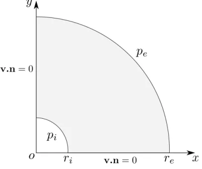
4.8 Domain of study and boundary conditions for the radial flow . . . 95

4.9 Isovalues of velocity for radial flow, (Figure 4.8) . . . 96

4.10 Isovalues of pressure for Darcy flow, (Figure 4.8) . . . 96

4.11 Comparison between analytical solution and numerical solution of pressure for the radial flow, (Figure 4.8) . . . 97

4.12 Convergence of the error for (a) the pressure and (b) the velocity for Darcy problem, with µ = 1P a.s, k = 1m2 _{. . . .} ₉₉

4.13 Isovalues of pressure and velocity for Darcy problem, with µ = 1P a.s, k = 1m2_,

h = 0.0125m. . . 99

4.14 Domain of study for the manufactured solutions for Stokes-Darcy coupled problem.100

4.15 Isovalues of pressure obtained with ASGS method (a) and with P1+/P1-HVM method (b) for µ = 1P a.s, k = 1m2 _{and α = 1} _{. . . 103}

4.16 Isovalues of velocity obtained with ASGS method (a) and with P1+/P1-HVM method (b) for µ = 1P a.s, k = 1m2 _{and α = 1} _{. . . 104}

4.17 Convergence of the error for the pressure and velocity in Stokes domain for Stokes-Darcy coupled problem with µ = 1P a.s,k = 1m2_{,α = 1.}_{. . . 105}

4.18 Convergence of the error for the pressure and velocity in Darcy domain for Stokes-Darcy coupled problem with µ = 1P a.s,k = 1m2_{,α = 1} _{. . . 106}

4.19 Computational domain of perpendicular flow and associated boundary conditions107

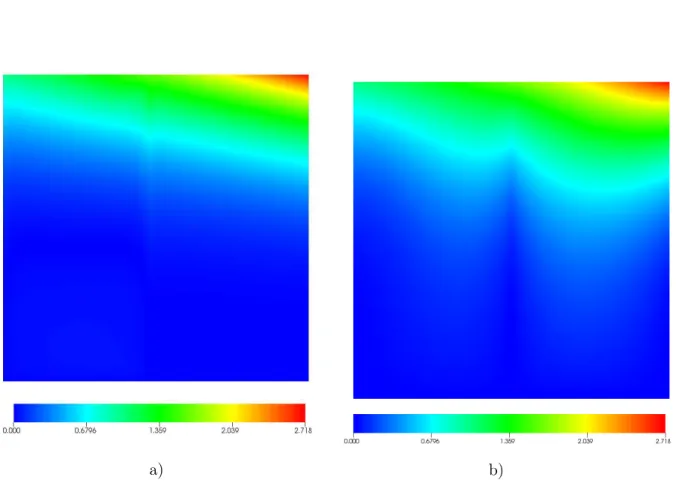
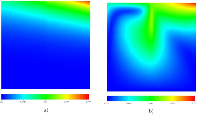
4.20 Comparison of velocity in perpendicular flow test between ASGS method and P1+/P1-HVM method, with k = 10−11_m2_{, µ = 1P a.s, p = 10}5_{P a and α = 1}_{. . 108}

4.21 Comparison of velocity in perpendicular flow test between ASGS method and P1+/P1-HVM method, with k = 10−14_m2_{, µ = 1P a.s, p = 10}5_{P a and α = 1}_{. . 109}

4.22 Normalized normal velocity vy for viscosity µ = 1P a.s with different

permeabil-ities and α = 1 . . . 110

4.23 Isovalues of pressure for perpendicular flow with k = 10−14_m2_{, p = 1 bar, µ =}

1P a.s and α = 1 . . . 111

4.24 Isovalues of pressure for perpendicular flow in 3D with k = 10−14_m2_{, p = 1 bar,}

µ = 1P a.s and α = 1 . . . 112

4.25 Isovalues of velocity for perpendicular flow in 3D with k = 10−14_m2_{, p = 1 bar,}

µ = 1P a.s and α = 1 . . . 113

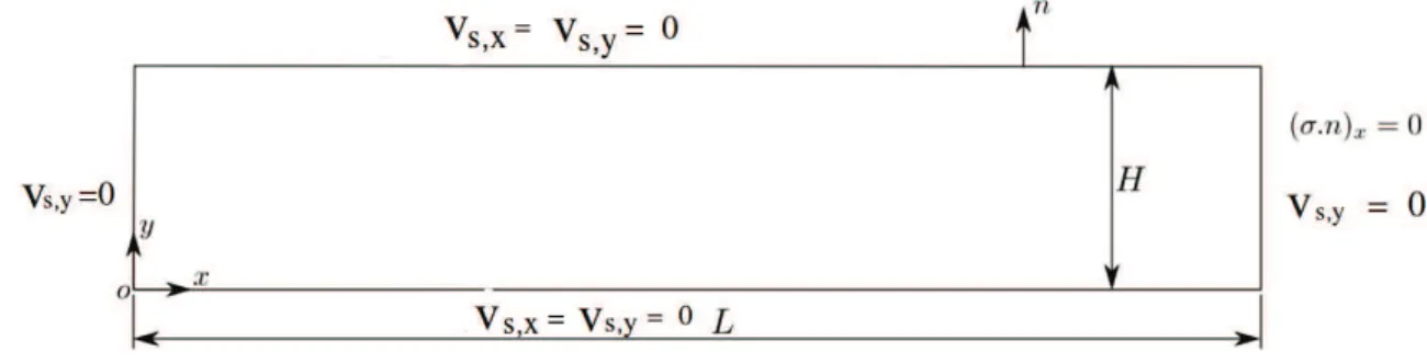
4.26 Computational domain for parallel flow and boundary conditions . . . 114

4.27 Isovalues of pressure (Pa) for parallel flow with k = 10−14_m2_{, µ = 1, α = 1 and}

(10)

4.28 Isovalues of velocity (magnitude-velocity m/s) for parallel flow with k = 10−14_m2_,

µ = 1, α = 1 and p = 105_{P a} _{. . . 115}

4.29 Comparison between analytical solution and numerical solution of Stokes veloc-ity for k = 10−14_m2_{, µ = 1, α = 1 and p = 10}5_{P a, 2D parallel flow.} _{. . . 116}

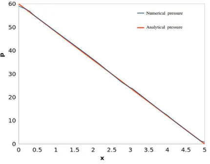
4.30 Comparison between analytical pressure, numerical pressure obtained with ASGS method and numerical pressure obtained with P1+/P1-HVM method for parallel flow with k = 10−14_m2_{, µ = 1, α = 1 and p = 10}5_{P a.} _{. . . 116}

4.31 Isovalues of pressure for parallel flow with k = 10−14_m2_{, µ = 1, α = 1 and}

p = 105P a. . . 117

4.32 Isovalues of velocity for parallel flow with k = 10−14_m2_{, µ = 1, α = 1 and}

p = 105P a. . . 117

4.33 Part of the computational domain of the interface-capturing test and zoom on the interface which cuts the elements . . . 118

4.34 Comparison of numerical solutions for monolithic approaches for a parallel flow, with analytical solution. Velocity is normalized by the maximum analytical velocity (vx,max,analytical). Interface reconstruction and Dirac approximation

for the surface integral are presented, k = 10−14_m2_{, p}

ext = 1Bar, µ = 1P a.s

and α = 1 . . . 119

4.35 (a) The mesh of the inclined domain with the interface (in red) which cuts the elements, (b) Computational domain with inclined interface and boundary conditions . . . 120

4.36 Isovalues of pressure (Pa) for ASGS method for k = 10−11_m2 _{. . . 121}

4.37 2D simulation for the 2D flow with inclined interface, (k = 10−11_m2_{, α = 1, µ =}

1P a.s, Pext= 1bar), magnitude-velocity (m/s). . . 121

4.38 Profil of pressure and velocity in the middle of the domain, x = 0.5m, k = 10−11m2, p = 1bar, µ = 1P a.s and α = 1. . . 122

4.39 Computational domain with curved interface . . . 124

4.40 Computation of the smallest distance between a node Mj and the segments of

the zero level set . . . 124

4.41 Isovalues of the level-set function between Stokes and Darcy, the black curve represents the isovalue zero of the level-set function (Stokes-Darcy interface). . 125

4.42 Isovalues of pressure, 2D flow with curved interface . . . 125

4.43 Isovalues of velocity, 2D flow with curved interface (m/s) . . . 126

(11)

List of Figures

4.45 Isovalues of velocity (m/s), 3D flow on a regular piece with injection channel . 127

4.46 The isovalue zero of the level-set function between Stokes and Darcy . . . 128

4.47 Isovalues of the level-set function between Stokes and Darcy. . . 128

4.48 3D simulation for the flow in 3D complex piece with curved interface, (k = 10−9m2, α = 1, µ = 1P a.s, Pext= 1bar) . . . 129

5.1 (a) definition of height function and (b) parametric interpolant [Hyman 1984] . 133 5.2 Actual geometry [M.Rudman 1997] . . . 136

5.3 (a) SLIC (x) and (b) SLIC (y). . . 136

5.4 (a) Hirt-Nichols and (b) Young-VOF . . . 136

5.5 Level set function . . . 138

5.6 Discretized level set function φh . . . 139

5.7 A complete turn of a circle using Cranck-Nicholson scheme . . . 147

5.8 Deformation of the circle: black line represents the initial position of the zero level set function, the red line represents the zero isovalue of the level set after one complete rotation using Cranck-Nicholson scheme and blue line represents the isovalue of the level set function after one complete rotation using implicit Euler scheme, (a) mesh: 50 × 50, ∆t = 0.01s, (b) mesh:50 × 50, ∆t = 0.005s . 147 5.9 Deformation of the circle: black line represents the initial position of the zero level set function, the red line represents the zero isovalue of the level set after one complete rotation using Cranck-Nicholson scheme and blue line represents the isovalue of the level set function after one complete rotation using implicit Euler scheme, (a) mesh: 100 × 100, ∆t = 0.005s, (b) mesh: 200 × 200, ∆t = 0.0008s. 148 5.10 Lagrangian description of the movement of the domain Ω . . . 150

5.11 Intermediate configuration Ωi _{. . . 155}

5.12 Compaction test . . . 159

5.13 Isovalue of the displacement uy . . . 160

5.14 Constitutive law of NC2 preforms in compaction [Celle et al. 2008] . . . 162

5.15 Compaction of a preform with free board. . . 165

5.16 Comparison between analytical and numerical results of the node position in the compaction test with free boards . . . 166

6.1 Injection algorithm . . . 169

6.2 Infusion algorithm . . . 172

(12)

6.4 Geometry and boundary conditions of a plate with filled distribution medium . 174

6.5 mesh made up by triangles and Stokes-Darcy interface in red (2500 nodes and 5000 elements). . . 175

6.6 Results of a plate simulation with filled distribution medium. Air is shown in blue and resin is shown in red, k = 10−14_m2_{, ∆t = 100s.} _{. . . 176}

6.7 Position of the resin front in function of time . . . 177

6.8 The filling time as a function of permeability in log-log scale with a slope equal to 1 . . . 178

6.9 Geometry and boundary conditions . . . 179

6.10 Zoom on the fluid medium and the porous medium mesh and Stokes-Darcy interface in red . . . 180

6.11 (a) Pressure distribution, (b) velocity distribution for a permeability k = 10−14_m2₁₈₁

6.12 2D simulation of resin injection with filling the distribution medium for k = 10−14m2, and a distribution medium thickness equal to 3mm. The resin is represented in red and the air is represented in blue. . . 182

6.13 2D simulation of resin injection with filling the distribution medium for k = 10−14m2, and a fluid medium thickness equal to 30 mm. The resin is represented in red and the air is represented in blue. . . 183

6.14 2D simulation of resin injection with filling the distribution medium for k = 10−8_m2_{, and a fluid medium thickness equal to 30 mm. The resin is represented}

in red and the air is represented in blue. . . 184

6.15 3D simulation of resin injection with filling the distribution medium for k = 10−13_m2_{. The resin is represented in red and the air is represented in blue.} _{. . 186}

6.16 Geometry and boundary conditions of a 2D complex piece with A = 0.1 m, C = 0.1 m, D = 0.04 m and β = π₄ . . . 187

6.17 mesh of the 2D complex piece made up of 3213 nodes. . . 187

6.18 2D simulation of resin injection with filling of the distribution medium for k = 10−7m2. The resin is represented in red and the air is represented in blue. . . . 188

6.19 2D simulation of resin injection with filling the distribution medium for k = 10−14m2. The resin is represented in red and the air is represented in blue. . . 189

6.20 (a) Pressure distribution and (b) velocity distribution for a 2D simulation of a complex piece . . . 190

(13)

List of Figures

6.22 3D simulation of resin injection with filling the distribution medium for k =

10−13_m2_{. The resin is represented in red and the air is represented in blue.} _{. . 192}

6.23 Zoom on the filling default located in the bottom of the complex piece where the resin has a radial flow . . . 192

6.24 (a) velocity distribution, (b) pressure distribution for a 3D simulation of a com-plex piece with a permeability k = 10−13_m2 _{. . . 193}

6.25 Boundary conditions of a plate infusion with filled distribution medium for the solid mechanics problem (a) and for the fluid mechanics problem (b) . . . 194

6.26 A zoom on the coarse mesh of this plate with the Stokes-Darcy interface in black color . . . 195

6.27 A zoom on the compaction of the plate with filled distribution medium, (a): before compaction, (b): after compaction, (c): during resin infusion . . . 196

6.28 Change of the preforms thickness after compaction (b) and after infusion (c) . . 199

6.29 Change in the porosity after preforms compaction (a) and after resin infusion (b)200 6.30 Evolution of preforms thickness after compaction and after resin infusion . . . . 200

6.31 Infusion of a plate with LRI process . . . 201

6.32 The mesh of the domain made up of 2300 nodes . . . 202

6.33 Boundary conditions of the solid mechanics problem (a) and of the fluid me-chanics problem (b) . . . 202

6.34 2D simulation of preform infusion at the initial time, (a) after compaction, (b) after a total filling of distribution medium and (c) after the total filling of preforms203 6.35 3D simulation of resin infusion process with filling distribution medium, Stokes-Darcy interface is shown in green and the fluid flow front in red. (a): Initial state (b): after compaction (c) −→ (e): evolution of resin flow front. . . 204

6.36 (a) pressure distribution during compaction (b) pressure distribution after resin infusion . . . 205

B.1 Representation of three rectangles. . . 213

B.2 Definition of a rectangle R . . . 214

B.3 Distance from a node M to a rectangle R . . . 215

B.4 Different possible areas . . . 215

B.5 Isovalue of the level set function which represents Stokes-Darcy interface in 2D. The Stokes-Darcy interface is represented in red . . . 216

B.6 Isovalue of the level set function which represents Stokes-Darcy interface in 3D. The Stokes-Darcy interface is represented in red . . . 216

(14)

C.1 Boundary conditions of a plate infusion with filled distribution medium for the solid mechanical problem (a) and for the fluid mechanical problem (b) . . . 217

C.2 2D simulation of NC2 preforms with 48 plies. The resin is shown in red and the air is shown in blue . . . 218

(15)

(16)

1.1 Comparison of different types of fibers [Dursapt 2007]. . . 8

4.1 Errors of velocity and pressure for the Stokes problem . . . 93

4.2 Errors of velocity and pressure in Darcy’s domain . . . 98

4.3 Errors for velocity and pressure in norm L2 _{for both ASGS and P1+/P1-HVM} methods in Stokes domain . . . 102

4.4 Errors for velocity and pressure in L2 _{norm for both ASGS and P1+/P1-HVM} methods in Darcy’s domain . . . 102

4.5 Relative errors for normal velocities in Stokes and Darcy regions, ASGS method and P1+/P1-HVM, k = 10−14 _m2_{, perpendicular flow.} _{. . . 111}

5.1 CPU times and conservation of the mass of fluid for different size of mesh and time step in the simulation of the rotation of the circle, the conservation is the difference between the final t = 1 and the initial surface of the circle. . . 148

5.2 Measures of deformations . . . 152

5.3 Comparison between analytical and numerical results . . . 160

6.1 Physical parameters of the numerical simulation. . . 175

6.2 Values of the relative errors of the filling time, and values of the CPU time of the simulation with respect to the time step . . . 178

6.5 Initial conditions of experimental and numerical simulation of 24 plies infusion. 198 6.6 Comparison between numerical and experimental results obtained after the com-paction of 24 plies . . . 198

6.7 Comparison between analytical and experimental results obtain after the infu-sion of 24 plies . . . 198

C.1 Physical parameters of the numerical simulation. . . 218

C.2 Comparison between numerical and experimental results obtained after the com-paction of 48 plies of NC2 preforms . . . 219

(17)

List of Tables

C.3 Comparison between experimental and numerical results obtained after the in-fusion of resin into 48 plies of NC2 preforms . . . 219

(18)

The use of composite materials has spread during the last decade, especially in aeronautics and automotive. The best known example is probably the Airbus A380 aircraft, of which about 25 % of the mass is composed of composite materials. Composite materials considered here, are obtained by a combination of an organic matrix, which ensures the cohesion of the material, and fiber reinforcement (fibers of carbon, glass fibers, etc..) that gives the material its mechanical properties . The advantage of composite materials is that they have high properties weight ratio compared with metals. Composite materials take part in the reduction of the weight of the structures, allowing the reduction of the energy transportation costs. In addition, composite pieces can be tailored in such a way that their reinforcement direction permit to deal with the multi-directional mechanical sollicitations.

However, several obstacles may affect the use of composite materials, their costs and more generally their development. Usually, we distinguish two types of manufacturing processes: wet processes and dry processes. In wet processes, fiber reinforcements are sold pre-impregnated with resin. This makes easier the development of the piece, and provides a good control of the fiber fraction, which is of paramount importance in composite materials performance. How-ever, these processes are expensive because they require refrigerated storage of pre-impregnated reinforcements and heavy hand costs. To reduce this cost, wet processes have been developed in the last years. They consist in infusing the resin into fibrous preforms during the manufac-turing process. However, the control of these processes is more difficult, it is hard to control the most critical properties related to the final piece like the volume fraction of fibers. For this reason, this work is conducted to propose a numerical methodology to simulate the resin infusion process which will help to control them and therefore to tune the process parameters to control the final piece geometrical as well as physical properties

Especially, we are interested in manufacturing large pieces. In this case, the resin is fed over the preforms (not impregnated yet) in a fluid distribution medium of a very high permeability. Then, under the action of mechanical pressure, exerted by the atmosphere when the vacuum is pulled, the resin is infused in the thickness of preforms. The complete modelling of this process is very complex and involves several physical phenomena. First, the dry preforms are compacted, and undergoing also large deformations. The thermoset resin flows then in the fluid distribution medium then into preforms. During its infusion, the resin undergoes, during

(19)

List of Tables

its infusion thermochemical transformations that affect its viscosity. The pressure applied by the resin into fibers network causes the inflation of preforms which modifies their porosity and therefore their permeability. This phenomenon is observed when coupling solid and fluid me-chanics.

Moreover, one should take into consideration the cooling phase, during the development of internal stress. However, in this work, we have isothermal conditions and the resin is considered as Newtonian incompressible fluid with constant viscosity. We model the flow of resin into the fluid distribution medium using Stokes’ equations. The flow of resin into preforms is described by Darcy’s equations with low permeability of order 10−14_m2_{. The deformations of wet and}

dry preforms are considered with an elastic non linear law.

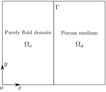
An important part of this work is dedicated to solve, using the finite element method, Stokes-Darcy coupled problem. This work is based on the work of Guillaume Pacquaut which defended his phd at École Nationale des Mines de Saint-Étienne in december 2010. Following this work, we adopted a monolithic approach for the Stokes-Darcy coupled problem, which means that we use one single mesh for Stokes and Darcy. The interface which separates these two domains is represented by the isovalue zero of a level set function φ defined as a distance function to the interface. The coupled problem is classically solved by formulating first a mixed velocity-pressure problem. It is known, relatively to Brezzi-Bab˜uska theory that the pair of the chosen interpolations should mainly satisfy two conditions (V0 ellipticity of a and the inf-sup

condition on b in their classical notations) which conducts to a discrete problem well-posed (existence and unicity of the solution). The difficulty of the choice of stable elements for Stokes-Darcy coupled problem is that the stable elements for Stokes are not stable for Darcy and vice versa. Therefore, the inf-sup condition presents a problem in the choice of the pair of elements in Stokes, especially in the choice of pressure space while the problem in Darcy is the V0ellipticity condition and the control of the divergence of the velocity. Briefly, it does not exist

a standard stable finite element pair for both Stokes and Darcy. The choice of different stable pairs (defined in two different discretized spaces) succeeds in decoupled approach where every domain is represented by a mesh independently from the other domain. However, in a mono-lithic approach, this is not possible because it conducts to a loss of consistency of the solution and oscillations around the interfaces. This is the limitation of the approach proposed by Guil-laume Pacquaut which relies on the MINI-element in Stokes (linear elements for velocity and pressure, the velocity is enriched by a bubble function) and a linear element for pressure and

(20)

velocity in Darcy stabilized with a Variational MultiScale method (Hughes Variational Mul-tiScale). This pair of elements (P1+/P1-HVM) does not ensure the continuity of the normal velocity on the interface (consistency error) and leads to oscillations of velocity on the interface. In this work, velocity and pressure fields, in Stokes and Darcy are approximated by linear and continuous functions per element (triangle or tetrahedron). The pair P1−P1(linear-linear)

is not stable for Stokes and Darcy. For this reason, we modify the discrete variational formu-lation of the problem by adding additionnal terms depending on the size of mesh and residual finite elements to make them stable. In addition, we use stabilization methods called "Vari-ational MultiScale". Developed twenty years ago, these methods offer a generic and formal framework for the stabilization of the finite elements formulations. They consist in decompos-ing the unknown and the test functions of the problem into two components: one corresponddecompos-ing to the unresolvable scale which is not captured by the mesh and another one corresponding to the resolvable scale which is the finite element solution. After this step, we establish fine scale problem and coarse scale problem (finite element problem). The approximation of the fine scale problem is injected in the finite element problem which allows the generation of stabilization terms.

When the Stokes-Darcy coupled problem is solved, we use it for the simulation of resin infusion processes, where the thickness of the fluid distribution medium is very low relatively to the thickness of the piece, and the permeability of fibrous reinforcement is small. The second level set function is used to describe the moving flow front, this function is initially defined by hyperbolic tangent form of the signed distance function to the resin front, and is constant outside a neighbourhood of this front. We adopt an Updated Lagrangian approach to solve the solid mechanics problem, i.e the deformation of dry preforms under their compaction due to a mechanical pressure and the deformation of wet preforms due to the pressure of the infused resin. The coupling between the resin flow and the deformation of preforms is carried out incrementally via the pressure of the resin in the expression of the wet preforms mechanical response, then via the porosity and the permeability which is a parameter present in Darcy’s equations.

Our manuscript is organized as follow:

– The first chapter introduces the definition of composite materials with organic matrix and their manufacturing processes. Then, we concentrate on the description and the

(21)

List of Tables

modelling of the process that we take into consideration which is "LRI" (Liquid Resin Infusion)

– The second chapter is an essential bibliographic study concerning the mixed finite ele-ments used to solve Stokes’and Darcy’s equations and then Stokes-Darcy coupled prob-lem. We introduce the theoretical framework of Brezzi-Bab˜uska which allows to establish the conditions of existence, unicity and stability of the solutions of both the discrete and continuous problem.

– The third chapter presents the method that we choose to couple Stokes and Darcy in a single approach: the finite element formulation is stabilized by using Variational MultiScale method called "ASGS" method (Algebraic SubGrid Scale). An analysis about the constants of stabilization which appear in this method is carried out.

– The fourth chapter is dedicated to the numerical validation of Stokes-Darcy coupled problem using ASGS method in the conditions imposed by LRI process. Different tests are conducted to validate the coupling conditions on the interface, such as a flow per-pendicular to the interface, a flow parallel to the interface, and we use the manufactured solution method to study the order of convergence. In addition, we compare the ob-tained results with those obob-tained by another monolithic approach and by a decoupled approach.

– The fifth chapter is made up of two distinct parts. In the first part, we present a bib-liographic study of the numerical methods of interface capturing. After this, we detail the method chosen to model the fluid front, the level set method combined with a hyper-bolic tangent filter. In the second part of this chapter, we deal with the deformation of preforms. We introduce the theoretical context of large deformations, then we formulate the mechanical problem with a Lagrangian Updated approach. Finally, we formulate the coupling between the deformations of preforms and the flow of the resin into preforms – The sixth chapter proposes some simulations of resin injection (Stokes-Darcy and level

set) then the infusion of resin (Stokes-Darcy, level set and deformation of preforms). 2D and 3D simulations are considered on simple cases, and then on complex pieces presenting curvatures and thickness. A comparison with existing experimental results is proposed on a simple geometry.

(22)

Composite materials, LCM processes

and their modelling

Contents

1.2 Composite materials constituents . . . 6

1.2.1 Matrix . . . 6

1.2.2 Reinforcements . . . 7

1.3 Manufacturing processes of composite materials . . . 9

1.3.1 Dry route processes . . . 9

1.3.2 Wet route processes . . . 10

1.4 Industrial context . . . 12

1.5 Challenges and motivation of this work . . . 12

1.6 Modelling scales . . . 13 1.6.1 Microscopic scale . . . 13 1.6.2 Mesoscopic scale . . . 14 1.6.3 Macroscopic scale. . . 14 1.7 Multi-domain modelling . . . 14 1.8 Multi-phyiscal modelling . . . 15 1.9 Conclusions . . . 17

(23)

1.1. Introduction

1.1 Introduction

Composite materials consist of a combination of materials that are mixed together to achieve specific structural properties. A composite material is made of a reinforcement material embed-ded in a resin matrix. The properties of the composite material are superior to the properties of the individual materials from which it is constructed. The main advantages of composite materials are their high strength and stiffness, combined with low density, when compared with bulk materials, allowing for a weight reduction in the finished part. Composite materials have gained popularity (despite their high cost) in high performance products that need to be lightweight and "strong" enough such as aerospace structures, tails, wings, fuselages, bicycle frames and racing car body (Figure 1.1). In the first part of this chapter, we will introduce composite materials properties and their manufacturing processes. Then, we will detail the resin infusion processes that we will model and show the difficulties related to their modelling. In the second part of this chapter, we will present the modelling of resin infusion processes taking into consideration the coupling between different physical phenomena occuring in resin infusion processes.

Figure 1.1: Composite materials products: (a) GD - Aston Martin V12 Vanquish, (b) HP - Boeing 787 Dreamliner

1.2 Composite materials constituents

1.2.1 Matrix

Synthetic resins are used as matrix materials in organic composites. Resins are generally either thermoplastic resins or thermosetting resins.

Thermosetting resins are the most diverse and widely used of all man-made materials. They are linked together by tight bounds of a chemical nature. After their polymerization by

(24)

ap-plying heat in the presence of a catalyst, these resins lead to geometric structure that can be destroyed only by a considerable application of thermal energy. For this reason, thermoset-ting resins have high thermomecanical properties. The principal thermosetthermoset-ting resins used in manufacturing composite materials are polyethanes, polyester and epoxy. Epoxy resins are the most widely used in high-performance composites. Polyester resins are the most widely used because of their low production cost, their flexibility and their stiffness.

In thermoplastic resins, macromolecular chains are linked together by weak bonds of physical nature. The advantage of thermoplastic resins lies in their low cost and recyclability. Nev-ertheless, this low cost is associated with low thermomechanical and mechanical properties. Their mechanical applications include helicopter rotor blades, and fairing panels on civil air-crafts. The most commonly used contemporary compounds are polyethylene, polyester and polycarbonate.

1.2.2 Reinforcements

Reinforcements bring to the composite material its mechanical properties [Berthelot 2005]. They are commercialized in the form of preforms of various architectures which can be dry or pre-impregnated with resin. Fibers are the most commonly used reinforcements. There are different types of fibers: Carbon, Glass fibers and Aramid fibers which can be purchased in various formats (chapped fibers, long fibers, fiber tows · · · ).

Glass fibers and Aramid fibers

Glass fibers are often used for helicopter rotor blades, for secondary structure on aircraft such as fairings and wings tips. Glass fibers have lower cost than other fibers. Composite materials made up by Glass fibers are available as a dry fabric or prepreg material. There are several types of Glass fibers: E-glass,D-glass,C-glass, R or S glass.

– E-glass accounts for 90 % of the glass fiber market and is used mainly in a polyester matrix and it has good electrical properties.

– D-glass has high dielectric properties. – C-glass has good chemical resistance.

– R-glass or S glass has high mechanical resistance.

Aramid fibers are light weight, strong and tough [Dursapt 2007]. Aramid fibers have high resis-tance to impact damage, however, they are weak in compression due to the interface weakness. The most well-known and used aramid fibers is Kevlar.

(25)

1.2. Composite materials constituents

Carbon fibers

Carbon fibers are the dominant advanced composite materials for aerospace, automobile, sport-ing goods due to their high strength, high modulus, low density and reasonable cost. There are several types of Carbon fibers: fiber with high resistance (HR), fiber with intermediate mod-ulus (IM) and fiber with high modmod-ulus (HM). Table 1.1allows to compare the characteristics of the different types of fibers.

Preforms architecture

The diameter of fibers is small, for this reason, preforms are commercialized in different forms of products which contain million of fibers, architectured in different forms. Several types of fibers architecture can be used depending on the number of directions occupied by fibers: Unidirectional (UD), bidirectional and multidirectional. Figure 1.2 shows the different types of preforms architecture.

Characteristics E-glass R-glass Carbon Carbon Aramide

HR HM

Young modulus

E (GPa) 73 85 240 400 135

Tensile strength

R (MPa) 3500 4500 3800 1600 3100

Compressive strength Medium Medium Good Good Bad Shock resistance Medium Medium Weak Weak Excellent

Sensibility

to humidity Yes Yes No No Yes

Density

2,6 2,6 1,75 1,9 1,5

Expansion coefficient

(10−6_mm/mm/C) ₅ ₄ ₁ ₁ ₀

Relative price 1 4 30 60 10

(26)

Figure 1.2: Different types of preforms architecture

1.3 Manufacturing processes of composite materials

Manufacturing processes for composite materials are numerous. They can be classified into two categories: dry route processes and wet route processes.

1.3.1 Dry route processes

Dry processes correspond to processes where composite material is formed by stacking “prepregs”. Prepregs are composite reinforcements (glass fibers, carbon fiber, aramid, etc.) that are pre-impregnated with resin. Dry processes have the advantage of convenient use and can easily master the final properties of the final product especially the volume fraction of fibers. The stacking of “Prepregs” is then placed in a mould for manufacturing the composite material. Prepreg materials are cured with an elevated temperature within an autoclave, oven or heat blanket. These processes allow to obtain composite pieces with excellent mechanical properties resulting from a low porosity and a high volume fiber fraction. However, the cost of storage is high because Prepreg material must be stored in a freezer at a temperature below 0◦ C to delay the curing process.

(27)

1.3. Manufacturing processes of composite materials

1.3.2 Wet route processes

These processes appear to reduce the costs with performance and properties identical to those obtained with dry processes. Wet processes are used for the development of composite materials in aeronautics, automative and shipbuilding.

There are two main types of processes. First there are processes based on injection of the resin into a mould like RTM (Resin Transfer Molding), VARTM (Vacuum Assisted Resin Transfer Molding) and ICRTM (Injection Compression Resin Transfer Molding).

Second, to solve the problems of filling met in manufacturing large pieces without high costs, infusion processes appeared twenty five years ago. The most known processes based on infusion of the resin are VARI (Vacuum Assisted Resin infusion), RIFT (Resin infusion under Flexible film infusion), LRI (Liquid Resin Infusion) and RFI (Resin Film Infusion). Below, we will describe RTM processes in the field of processes based on injection, LRI and RFI processes in the field of processes based on infusion.

1.3.2.1 RTM processes

Resin Transfer molding (RTM) is a composite manufacturing process in which fibrous pre-forms one placed in a closed mold, then a viscous resin is injected into the mold to fill the empty spaces between the network of fibers. Then a cycle of temperature is applied to allow the reticulation of resin taking place. The injection of resin occurs mainly in the plane of preforms. The pieces obtained with this process can be complex with a well controlled final thickness. However, it is important to achieve a large filling of the mold for large pieces. In this process, the vent location is one of the most important variable in process design, it has a great impact on mold filling time and resin flow pattern, which increases the process efficiency and the quality of products.

1.3.2.2 RFI (Resin Film Infusion)

RFI processes consist in depositing fibrous preforms under a layer of solid resin (Figure

1.3). A punched mold can be placed on the top of stacking to improve efficient finishing of the surface. The bleeder and a vacuum bag are placed on top of the assembly. Bleeder absorbs the mass of excess resin. First, a cycle of temperature is applied to maintain the resin in its liquid state and to allow the infusion of the resin through the preforms under the action of pressure cycle. Then, at the end of infusion, a cycle of temperature and pressure is applied again to lead to the crosslinking of the resin.

(28)

Figure 1.3: Resin Film Infusion (RFI) schematic 1.3.2.3 LRI processes (Liquid Resin Infusion)

In LRI processes, a resin bed is formed through a highly permeable fluid distribution medium placed on the top of fiber preforms. The deformation of the fluid medium is assumed to be negligible compared with the deformations into preforms due to its high stiffness distribution. A punched mold can be placed on the top of the stacking of preforms to improve the finishing of the surface which is not in contact with the mould (Figure1.4). A vacuum bag is then placed, and vacuum is pulled out to compact the stack of preforms. This also serves as a driving force for infusing the resin across the preforms. Indeed, the difference of pressure between the resin inlet, located in the fluid distribution medium, and the vacuum vent, set on the base of the preform, causes the infusion of resin into the fluid medium then across the thickness of preforms. When the infusion is complete, a cycle of pressure and temperature is applied to realize the crosslinking of the resin.

(29)

1.4. Industrial context

1.4 Industrial context

Resin infusion processes have been developed in recent years. They show an advantage rel-atively to "Prepregs" processes which have high storage costs and are limited to small pieces. Resin infusion processes allow a manufacturing of large pieces because they consist in infusing resin across the thickness of preforms rather then in their plane. Distances travelled by resin are small compared with the distances that are involved in processes by injection (RTM) and a good impregnation of resin is ensured which permits to obtain pieces with good mechanical properties. However, in LRI processes, some mechanical (thickness of preforms) and geometri-cal properties (fiber-volume fraction) are not well controlled. Numerigeometri-cal simulation will allow a better understanding of the influence of the LRI process parameters (pressure, temperature, viscosity, permeability) onto the final piece characteristics. This will lead to drastic reduction in turning these promissing manufacturing processes, and eventually to optimize the industrial process configurations.

1.5 Challenges and motivation of this work

Numerical simulation is necessary to optimize process promotion to reach infusion time and to master, above all, thickness and fibers volume fraction. Infusion process is a very complex problem to solve, it must rely on general model which couples all the mechanical (solid-fluid) and thermochemical phenomena. Decoupled representation of each phenomenon does not represent the physical reality. The difficulties met in this work is to model the isothermal flow of resin into preforms undergoing large deformations through two coupled mechanisms: the flow of resin (developed in chapter 2) and the deformation of preforms (developed in chapter 5). The second difficulty is the conservation of the fluid mass and the capture of moving flow fronts. To represent the moving flow front, we have two approaches. Lagrangian approaches where the moving flow front is presented by marks which correspond to the nodes of the boundary of the mesh. These marks change their position over the time with a velocity equal to the velocity of the resin. Eulerian approaches where the mesh is fixed. The front of the resin passes through the mesh and is represented by a function computed in the domain. In this case, we have to solve transport equation to detect the evolution of the resin flow front. Consequently, to simulate the resin infusion processes taking into consideration all the physical problems already cited, one has to propose a numerical multi-physical model able to describe the flow of resin into preforms undergoing large deformations. To this day, two models exist, one developed by Celle [Celle et al. 2008] and one developed by Pacquaut [Pacquaut 2009]. Celle uses a decoupled

(30)

approach which consists in using two different meshes matching at the interface which separate the resin (fluid) and the preforms (porous). Pacquaut uses a monolithic approach which consists in using one single mesh for resin and preforms and represents the interface between porous and fluid domains with a level set function. The numerical model developed by Pacquaut presents some accuracy problems such as consistensy errors and oscillations of velocity in severe cases corresponding to physical reality (complex geometries, curved interfaces and low permeabilities). The aim of this work, based on the work from Pacquaut is to propose a robust numerical multi-physical model to simulate resin infusion processes in an industrial context by using one mesh for resin and preforms. This model will be able to deal with physical and numerical problems met in literature [Pacquaut 2009] and to deal with severe cases matching with industrial reality.

Conclusions

We introduced in this first part, composite material and their manufacturing processes. In addition, we presented resin infusion processes which are hard to control (thickness of preforms, fiber-volume fraction). The numerical simulation will allow to understand this process and to reduce the costs of experimental turning. To understand the simulation methods, we will introduce in the next part the ways of modelling resin infusion processes.

1.6 Modelling scales

Composite materials are heterogenous materials consisting of fibers and resin. The first step implied to model these materials is to choose the scale of description of the physical mechanisms. In general, the more the modelling scale is low, the more we get close to the fundamental physical problem and the less we have to determine experimental parameters. However, the lower the modelling scale, the more we must have local meshes and inducing higher computational costs. There are several possible approaches: microscopic, mesoscopic and macroscopic approaches. Figure 1.5 illustrates these different scales in the case of a flow of resin through a fiber bed.

1.6.1 Microscopic scale

The microscopic scale corresponds to the scale where one is able to describe the flow of resin between the filaments (Figure1.5). Due to the large difference between the diameter of a fiber (7 − 10 µm) and the dimensions of a composite piece (of the order of a meter), this scale is usually not considered in simulation methods. In this approach, we use a representative

(31)

1.7. Multi-domain modelling

Figure 1.5: The different modelling scales of resin infusion processes

elementary volume (VER). This approach allows an accurate characterization of the behavior of fibers and resin because it consists in studying separatly their behavior using local models. However, this approach is difficult to implement in the case of industrial applications since the computation time associated with such models is prohibitive.

1.6.2 Mesoscopic scale

The mesoscopic scale is the scale where one is able to describe the flow of resin between the tows (Figure 1.5). The working scale corresponds to the tow dimension, typically one to several millimetres.

1.6.3 Macroscopic scale

The macroscopic scale corresponds to the scale of the piece, the tows are not represented and the stacking of tows is considered as a homogeneous equivalent medium (Figure 1.5). This approach is more convenient for the industrial cases. Indeed, the time of computation associated with these models is generally lower than the time associated with microscopic models. However, the physical characteristics of the enviromnent are complex to characterize and difficult to observe. To study the influence of process parameters ( pressure, temperature) on the final piece characteristics, we will use macroscopic approach to model resin infusion process through reinforcements represented as equivalent homogeneous medium.

1.7 Multi-domain modelling

Taking into account, the description of LRI process, we will adopt Multi-domain modelling described in Figure1.6where we decompose our domain into three different zones corresponding to:

(32)

– The fluid distribution medium corresponding to the draining fabrication so-called "Stokes zone".

– Preforms impregnated with resin (wet preforms).

– Preforms not impregnated yet with resin (dry preforms).

Figure 1.6: Representation of the domain decomposition into three zones during the modelling of resin infusion processes: fluid distribution medium with resin, dry preforms and wet preforms

1.8 Multi-phyiscal modelling

Resin infusion processes involve several complex physical phenomena. In reality, resin infusion process modelling consists in modelling and coupling four physical problems: fluid mechanics problem, solid mechanics problem, thermal problem, and resin cross-linking problem. Figure 1.7 illustrates the different physical phenomena and the interactions between these phenomena.

Fluid mechanics problem corresponds to the flow of resin in the fluid distribution medium and into preforms. This problem is coupled with the thermal transfer and the cross-linking kinetics. The cross-linking of resin affects the viscosity, then it affects the flow. This problem is coupled with the solid mechanics problem because it influences the deformation of preforms due to the pressure of the resin inside the pores. On the other hand, the solid mechanics problem influences the flow of resin because it changes the permeability of preforms i.e the capability of the preforms to be infused by the resin. Thermal and cross-linking problems are

(33)

1.8. Multi-phyiscal modelling

Figure 1.7: Physical phenomena occuring in the modelling of resin infusion processes

also important to model. The cross-linking changes the viscosity, then it affects the resin flow. In addition, cross-linking influences the thermal transfer because it produces heat during the resin exothermal polymerization. Converse, thermal transfer influences the cross-linking kinetic because the temperature is essential for the activation of the resin polymerization reaction. The temperature has also an effect on the resin flow because it changes the viscosity and affects the deformation of preforms by expansion.

In this work, we will concentrate on ﬂuid mechanics and solid mechanis without taking into consideration thermal and cross-linking aspects. In chapter 2, we will develop the modelling of ﬂuid mechanical problem and in chapter 5, we will develop the modelling of solid mechanics problem.

(34)

1.9 Conclusions

In this chapter, composite materials and their manufacturing processes were briefly de-scribed to define the general context of our work. Then, we presented the numerical simulation considered as an essential way to control resin infusion processes, especially the impregnation of resin into deformable preforms, which will allow to reduce the costs in turning composites materials manufacturing. In addition, we described briefly the bibliographic study of the mod-elling of resin infusion processes, taking into consideration all the physical phenomena included in this modelling. In the next chapter, we will describe the physical and mathematical models to describe the flow of resin in the fluid distribution medium and preforms, and the different stabilized methods used to discretize the associated mathematical model using finite element methods.

(35)

(36)

Stabilized finite element methods for

Stokes, Darcy and Stokes-Darcy

coupled problem

Contents

2.2 Stokes-Darcy coupled problem: strong and weak formulations . . . . 20

2.2.1 Modelling of the fluid part. . . 20

2.2.2 Flow of resin into preforms . . . 23

2.2.3 Stokes-Darcy coupled problem . . . 26

2.3 Stability of the mixed continuous and discretized problems . . . 31

2.3.1 Stability of the mixed continuous problem . . . 31

2.3.2 Stability of the Galerkin discretized mixed problem. . . 35

2.4 Mixed stable and stabilized finite elements for Stokes problem . . . . 37

2.4.1 Stable mixed finite elements . . . 38

2.4.3 Multiscale Methods . . . 44

2.4.4 Stabilized finite element methods based on multiscale enrichment of Stokes

problem and Petrov Galerkin approximation . . . 45

2.5 Stabilized finite elements for discretization of Darcy’s equations . . . 48

2.5.1 Stable mixed elements . . . 49

2.5.3 Multiscale Methods . . . 51

2.5.4 Galerkin Least Squares methods . . . 53

2.6 Stabilized finite elements for Stokes-Darcy coupled problem . . . 56

(37)

2.1. Introduction

2.1 Introduction

In this chapter, we will present the modelling of the resin flow, the resin being considered as an incompressible fluid. It consists on modelling the resin into the fluid distribution medium and into preforms. We present separately Stokes equations and Darcy equations. Then, we present the discretized finite element method used for Stokes and Darcy, and the different stabilized methods used in the literature which lead to stabilize the Galerkin’s formulation of Stokes and Darcy’s equations. Then, we present the "unified" and "decoupled" strategies used in coupling Stokes and Darcy flows and the way to choose compatible finite elements for both Stokes and Darcy in the coupling problem.

2.2 Stokes-Darcy coupled problem: strong and weak

formula-tions

In this section, we will present the modelling of the fluid. For that we first introduce Stokes’ equations and their weak formulation. Then, we present the modelling of the resin flow into preforms. For this we introduce Darcy’s equations and their weak formulation. Finally, we present the Stokes-Darcy coupled problem and its weak formulation.

2.2.1 Modelling of the fluid part

2.2.1.1 Incompressible Newtonian fluid

The first assumption is related to the resin which is classically considered as a Newtonian incompressible fluid:

σs = 2µ ˙ε(vs)− psI (2.1)

where σsis the cauchy stress tensor, ˙ε(vs) is the strain rate tensor which is defined by ˙ε(vs) = 1

2(∇vs+∇vsT), vs is the resin velocity, ps is the hydrostatic pressure, µ is the viscosity and

I is the second order identity tensor.

2.2.1.2 Stokes equations

Let us consider Ωs the region occupied by the fluid, the motion of which is described by

both the momentum and mass balance equations. We consider ∂Ωs the boundary of Ωs that

can be split into two distinct parts, ∂Ωs = Γs,D∪ Γs,N with Γs,D∩ Γs,N =∅, corresponding

(38)

natural condition. The velocity is enforced over Γs,D (Dirichlet condition), while the normal

stress is enforced over Γs,N (natural condition). The Stokes system, which expresses momentum

and mass balances when inertia effect is neglected, is written as: find the velocity vs and the

pressure ps fields defined by:

−div(2µ ˙ε(vs)) +∇ps = fs in Ωs

div vs = hs in Ωs

vs = v1 on Γs,D

σ_n,s ₌ _−p_ext,s_.n_s _{on Γ}_s,N

(2.2)

where fsis the volume force, v1 is the velocity prescribed on the boundary Γs,D, ns is the unit

vector normal to the boundary of Ωs and σn,s is the normal stress prescribed on Γs,N to be

equal to −pext,s.ns. If the fluid is incompressible then hs= 0.

2.2.1.3 Weak formulation of Stokes equations

In order to solve Stokes equations by the finite element method, the weak formulation has to be established. We introduce some spaces that we will use for the velocity, pressure and test functions in the weak formulation of Stokes equations:

Qs= L2(Ωs) ={u : Ωs→ R | Z Ωs u2dΩ <_∞} (2.3) H1(Ωs)m={u ∈ L2(Ωs)m | ∇u ∈ L2(Ωs)m×m} (2.4) Vs = HΓ1s,D(Ωs) m₌_{{u ∈ H}1_(Ω s)m| u = u1 on Γs,D} (2.5) Vs0= H_Γ1,t_s,D(Ωs)m={u ∈ H1(Ωs)m | u = 0 on Γs,D} (2.6)

L2(Ωs) is the Lebesgue space of square integrable functions and HΓ1s,D(Ωd)

m_{is the Sobolev}

space where m is the dimension of the problem (m = 2 or 3).

In the entire chapter, we note k.k0 and k.k1 the L2 and H1 norms defined by:

kqk0= (

Z

Ωs

(39)

2.2. Stokes-Darcy coupled problem: strong and weak formulations kwk1 = (kwk20+ m X j=1 k∂w ∂xjk 2 0)1/2

The weak formulation of Stokes problem is obtained by multiplying the Stokes Equation (2.2) by weighting functions ws ∈ Vs0 and qs ∈ L2(Ωs) and then by integrating by parts on the

domain Ωs. For the sake of simplicity, < ., . > denotes the scalar product of functions in

L2(Ωs).

The integration by part of the first term of the Stokes equation gives (Equation(2.2)):

− < div(2µ ˙ε(vs)), ws> = < 2µ ˙εij ∂ws,i ∂xj >− < 2µ ˙ε_ij_n_j_{, w}_s,i_>_Γ s,N = < 2µ ˙ε(vs) : ˙ε(ws) >− < (2µ ˙ε(vs).ns), ws>Γs,N (2.7)

Note_{: The integral < −2µ ˙ε(v}s).ns, ws >Γs reduces to < −2µ ˙ε(vs).ns, ws>Γs,N because the test function ws vanishes on Γs,D(w|Γs,D = 0).

The integration by parts of the second term of Equation (2.2) gives:

<_∇ps, ws>=− < ps, divws> + < ps, ws.ns>Γs with

< ps, ws.ns >Γs=< ps, ws.ns>Γs,N

since w_|Γ_s,D = 0.

Consequently, we obtain the weak formulation of Stokes equations: Find [vs, ps]∈ Vs× Qs such as:

< 2µ ˙ε(vs) : ˙ε(ws) >− < ps, divws>=<−pext,s.ns, ws>Γs,N + < fs, ws> (2.8) The weak formulation of Stokes equations can be written as:

Find vs∈ Vs and ps∈ Qs such that:

Bs([vs, ps], [ws, qs]) = Ls([ws, qs]), ∀ws∈ Vs0,∀qs∈ Qs (2.9)

The bilinear form Bs and the linear form Ls are defined by:

(40)

Ls([ws, qs]) =< fs, ws> + < hs, qs>− < pext,s.ns, ws>Γs,N (2.11) Let us note that this formulation corresponds to the dual weak formulation of Stokes equations.

2.2.2 Flow of resin into preforms

Ωdis the region occupied by the preforms. To model the infiltration of resin into preforms in

a macroscopic approach, one represents classically the preforms as an equivalent homogeneous porous medium. Consequently, the laws used to describe the flow into preforms are these from the mechanics of porous media, the classical laws proposed by Darcy [Darcy 1856] and Brinkman [Brinkman 1947]. The Reynolds number Re is the dimensionless number which

allows to simplify the modelling and measures the importance of the inertial forces compared with the viscous forces. It is written as Re = |vd| d ρ

µ where d is the average pore diameters, |vd| is the fluid velocity in the pores and ρ is the fluid density. The flow is considered as

laminar if the Reynolds number is much smaller than 1. Sometimes, it is difficult to know with precision the average pore diameter d. This is why some authors prefer to consider the root of the permeability1_{, denoted by}√_{k instead of d [}_{Bear 1990}_{]. In this case, the Reynolds number} can be written as: Re= vd

√ k ρ

µ . For more typical values corresponding to the case considered

in this work, vd = 1m/s, µ = 0.1P a.s, k = 10−14m2, ρ = 103Kg/m3 the Reynolds number is

equal to 10−3_{. Hence, the inertial forces are negligible compared with the viscous forces.}

2.2.2.1 Darcy’s law

The Darcy’s law is a derived constitutive equation that describes the flow of a fluid through a porous medium. The law was formulated by Henry Darcy [Darcy 1856], it is a simple first gradient proportional relationship between the volume flux (m/s) and the pressure change per unit length of the porous media. If the flow is one dimensional, the gradient of pressure is dp

dx,

the Darcy’s law is q = k µ

dp

dx. k is the permeability (m2), µ is the viscosity (Pa.s).

This law is convenient for a low Reynolds number (Re << 1), which is the case where

viscous forces dominate inertial forces. In this case, the gradient of pressure is proportional to the velocity of the fluid flow. This Darcy’s law can be generalized as [Hassanizadeh 1983]:

vd=−

k µ∇pd

with pd the pressure, k is the second order permeability tensor and vd the average of the

(41)

2.2. Stokes-Darcy coupled problem: strong and weak formulations

locity. To compute the actual fluid velocity in the pores, one has to divide vd by the porosity

ψ which is the ratio between the volume of pores and the total volume. Then, the real velocity denoted by vr is

vr =

vd

ψ

2.2.2.2 Brinkman’s law

An increasing number of articles use Brinkman’s equations in place of Darcy’s equation for describing flows in porous media. Brinkman’s law introduced in [Brinkman 1947] proposes to describe the flow into porous media by generalizing Navier-Stokes equations. This isotropic law for the flow of a Newtonian fluid through a swarm of fixed particles is in the form:

∇pd = −µ_kvd+ µe∆vd (2.12)

where µe_{is the effective viscosity (sometimes called "apparent viscosity"). The practical}

advan-tage of Equation (2.12) stands in the fact that it is a slight modification of Stokes equations. Theoretical investigations of the domain of validity of Brinkman equation yield to µe _{= µ}

[Vernescu 1990] and it is estimated that the effective viscosity µe _{goes to µ as the porosity}

increases to 1 which corresponds to important permeability while in resin infusion processes, on the contrary we have small permeabilities (10−8_m2_{≤ k ≤ 10}−15_m2_).

Both Darcy’s law and Brinkman’s law are valid at a large scale compared with the pore scale. It means they correspond to a macroscopic approach of the resin flow into preforms. In this manuscript, we will use Darcy’s equations considering the permability that we will use for preforms is typically between 10−8_m2_{and 10}−15_m2_.

2.2.2.3 Darcy’s equations

Let us consider Ωdthe region occupied by the preforms. We consider ∂Ωd the boundary of

Ωdthat can be split into two distinct parts ∂Ωd= Γd,D∪ Γd,N, corresponding to the two

differ-ent kinds of boundary conditions: Dirichlet and Newman. Respectively, the Darcy’s equations are then expressed as: