HAL Id: tel-01243560
https://tel.archives-ouvertes.fr/tel-01243560
Submitted on 15 Dec 2015HAL is a multi-disciplinary open access archive for the deposit and dissemination of sci-entific research documents, whether they are pub-lished or not. The documents may come from teaching and research institutions in France or abroad, or from public or private research centers.
L’archive ouverte pluridisciplinaire HAL, est destinée au dépôt et à la diffusion de documents scientifiques de niveau recherche, publiés ou non, émanant des établissements d’enseignement et de recherche français ou étrangers, des laboratoires publics ou privés.
example of gamma-ray bursts and supernovae
Anastasia Filina
To cite this version:
Anastasia Filina. Studying explosive phenomena in astrophysics by the example of gamma-ray bursts and supernovae. Other. Université Nice Sophia Antipolis, 2015. English. �NNT : 2015NICE4038�. �tel-01243560�
THESE
pour obtenir le titre de
Docteur en Sciences
de l’UNIVERSITE Nice Sophia Antipolis
Discipline : (ou sp´ecialit´e) Asrophysique Relativiste
pr´esent´ee et soutenue par AUTEUR Anastasia FILINA
Studying explosive phenomena in astrophysics by the
example of gamma
-ray bursts and supernovae
Th`ese dirig´ee par Pascal CHARDONNET soutenue le 01/07/2015
Jury:
Chardonnet Pascal LAPTH, Annecy-le-Vieux, France Directeur
Chechetkin Valery KIAM, Moscow, Russia Co-directeur
Chetverushkin Boris KIAM, Moscow, Russia Membre de jury
Della Valle Massimo OACN-INAF, Naples, Italy Rapporteur
Narozhny Nikolay MEPhI, Moscow, Russia Membre de jury
Pozanenko Alexei IKI, Moscow, Russia Membre de jury
Titarchuk Lev GMU - SPACS, Virginia, USA Rapporteur
Contents ii
List of Figures iv
List of Tables vii
Abstract viii
1 Introduction 1
1.1 Supernovae and gamma-ray bursts . . . 1
1.1.1 Observations . . . 3
1.1.2 Physical processes . . . 7
1.1.3 Nucleosynthesis . . . 9
1.2 Thesis outline . . . 10
2 Explosive phenomena in stellar physics 12 2.1 Different modes of combustion . . . 13
2.2 The role of instabilities . . . 24
2.2.1 Rayleigh-Taylor instability . . . 24
2.2.2 Landau-Darrieus instability . . . 26
2.2.3 Thermal-pulsational instability . . . 26
2.2.4 Pair instability . . . 27
3 Aspherical nucleosynthesis in a core-collapse supernova with 25 M⊙standard pro-genitor 28 3.1 Introduction . . . 28
3.2 Methods . . . 29
3.2.1 Piecewise Parabolic Method on a Local stencil for hydrodynamics . . . 29
3.2.2 Conjugate gradients for self-gravity . . . 30
3.2.3 Tracer particles method for nucleosynthesis . . . 30
3.3 Explosive nucleosynthesis . . . 31
3.3.1 Network of nuclear reactions . . . 31
3.3.2 Nuclear abundances . . . 33
3.3.3 Solving reaction network for nucleosynthesis . . . 34
3.4 SN model . . . 36
3.5 Results. . . 38
3.6 Conclusions . . . 46
4 Multidimensional simulations of pair-instability supernovae 49
4.1 Introduction . . . 49
4.2 Pair-instability supernovae . . . 50
4.3 Numerical approach. . . 51
4.3.1 Modelling in 1D . . . 52
4.3.2 Numerical explosion in multi-D . . . 54
4.4 Discussions and conclusions . . . 58
5 On GRB Spectra 59 5.1 Introduction: snapshot of GRB spectrum . . . 59
5.2 Black-body and Thermal Bremsstrahlung emission . . . 61
5.2.1 Our Model . . . 62
5.3 Analysis of gamma-ray bursts . . . 63
5.3.1 Analysis of GRB 090618. . . 63
5.4 Analysis of some other GRBs. . . 64
5.5 Discussions and conclusions . . . 67
6 Cosmology with GRBs 74 6.1 General introduction to cosmology . . . 74
6.2 Cosmology with GRBs . . . 81
6.3 Number of GRBs per redshift. . . 82
6.3.1 Luminosity function . . . 85 6.3.2 Rate of GRB . . . 86 6.4 Conclusions . . . 87 7 General conclusions 89 Analysis of some GRBs 91 Abbreviations 100 Physical Constants 101 Symbols 102 Bibliography 103 Acknowledgements 115
1.1 Supernova spectral types. Credit:Daniel Kasen . . . 5
1.2 A mosaic of HST images of the hosts of forty-two bursts (left) and the super-novae hosts (right) (Fruchter et al. 2006) . . . 6
1.3 Illustration of the light curves of a variety of supernovae on the left (Smith et al. 2007) and comparison it with GRBs on the right (Bloom et al. 2009). . . 7
1.4 Sample of light curves of bright BATSE bursts, showing high diversity. . . 9
2.1 Curves of constant shockwave velocity, called Rayleigh lines.. . . 14
2.2 The shock adiabatic or the Hugoniot adiabatic and Rayleigh line (dashed) .. . . 16
2.3 The detonation adiabatic (continuous line) and the ordinary shock adiabatic (dashed line). . . 18
2.4 The relation between the different modes of combustion . . . 22
2.5 Example of Rayleigh-Taylor instability simulations by the PPML code Popov (2012). The density map is shown . . . 25
2.6 Example of Landau-Darrieus instability simulations for the C/O flame (Bell et al. 2004). Inflow boundary conditions inject fuel into the bottom of the domain. The y-velocity of the material with respect to the planar flame is shown in color for different moments of time. . . 26
3.1 A simplified network of nuclear reactions from12Cto56Ni.. . . 32
3.2 Comparison of our nucleosynthesis computing code (on the top) and nucleosyn-thesis computing code from Timmes et al. (2000) (on the bottom). As an ex-ample we take evolution of the mass fractions under adiabatic expansion. The initial conditions are T = 3× 10⁹ K, ρ = 1× 10⁹ g cm−3and an initially half
12C- half16Ocomposition for the 13 isotope α-chain network. . . . . 35
3.3 Presupernova configuration. . . 36
3.4 Density distribution for t = 60.5 s after inducing the explosion. The coordinates are shown in the units of solar radius. Color represents the logarithm of density in the units of ρc =4.5× 10⁵g/cm3. . . 39
3.5 Temperature distribution for the same moment and in the same coordinate units as on fig. 3.4. Color represents the logarithm of temperature in the units of 109K. 39
3.6 Tracer locations and the density map for t = 60.5 s, reconstructed from the recorded tracers data. Color represents the temperature in the units of 109K. . . 40
3.7 Distribution of56Niand52Femass fractions in velocity map for t = 60.5 s. . . 41
3.8 Distribution of48Crand44T imass fractions in velocity map for t = 60.5 s.. . . 42
3.9 Distribution of40Caand36Armass fractions in velocity map for t = 60.5 s. . . 42
3.10 Distribution of32S and28S imass fractions in velocity map for t = 60.5 s. . . . 43
3.11 Distribution of24Mgand20Nemass fractions in velocity map for t = 60.5 s. . . 43
3.12 Distribution of16Oand12Cmass fractions in velocity map for t = 60.5 s. . . . 44
3.13 Distribution of4Hemass fraction for t = 60.5 s. The numbers show the values in some regions. . . 44
3.14 The schematic plot of main regions in the ejecta after explosion. . . 45
3.15 Comparison between the yields in our SN model (red line) and in a SN model of Maeda et al. (2002) (blue line). The total mass of the produced nuclei in the units of M⊙in logarithmic scale is shown. . . 47
4.1 Fate of a star depending on its mass, Mc, and binding energy, Ebind. Explosion
is marked by diamonds and collapse is marked by circles. . . 54
4.2 Nuclear energy release as a function of maximum temperature (diamonds). The slope E ∝ T2 is shown. For comparison data from Arnett (1996) (stars) and Ober et al. (1983) (triangles) are shown. . . 55
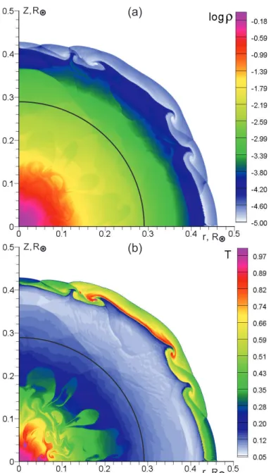
4.3 SN model with central ignition for t = 28 sec. Logarithm of density (a) is shown in units of ρc = 2.65× 10⁵ g/cm3. Temperature (b) is shown in units of
Tc =2.36× 10⁹K. . . 56
4.4 SN model with multicore ignition for t = 28 sec. Logarithm of density (a) is shown in units of ρc = 2.65× 10⁵ g/cm3. Temperature (b) is shown in units of
Tc =2.36× 10⁹K. . . 57
5.1 Time-integrated spectra GRB 090618 . . . 64
5.2 Time-integrated spectra for the different time intervals: from 0 to 50 s, from 50 to 59 s, from 59 to 69 s after the trigger time of GRB 090618. Blue line shows the fit with the Band function (Eq 5.1), orange line shows the blackbody +bremsstrahlung (Eq. 5.9). . . 65
5.3 Time-integrated spectra for the different time intervals: from 69 to 78 s, from 79 to 105 s after the trigger time of GRB 090618. Blue line shows the fit with the Band function (Eq 5.1), orange line shows the fit with blackbody + bremsstrahlung (Eq. 5.9). . . 66
5.4 The temperature evolution with time T(t) of GRB 090618 . . . 67
5.5 Example of light curve of GRB 090618 (Izzo et al. 2012) . . . 67
5.6 Hot spots randomly appear on the surface of exploding star. Each spot pro-duces spike of emission. Signals from these spots arrive at different times, so an observer sees the superposition of the spikes. . . 70
5.7 2D simulation of an explosion of a 100 solar mass pair instability supernovae ex-plosion in the multicore exex-plosion scenario using PPML methods. This picture shows the fragmentation of the core and hot spot regions of very high tempera-ture. . . 71
5.8 Cartoon representation of a possible emission mechanism with Black-Body + Bremmstrahlung emission . . . 72
6.1 Amati relation with redshift distribution . . . 82
6.2 Isotropic equivalent radiated energy from redshift Eiso(z) . . . 82
6.3 Comparison of luminosity distance computed from Amati relation” and from cosmological redshift by eq.6.42 . . . 83
6.4 ”Volumetric factor” dV/dz1+z (z) . . . 85
6.5 Integral of Luminosity Function from Campisi et al. (2010) and Wanderman & Piran (2010) . . . 86
6.6 Rate GRB from Hopkins & Beacom (2006) and rate PISN from Hummel et al. (2012) . . . 87
6.7 Number of observed GRBs with redshift in (z,z+dz) over a redshift interval . . 87
1 The temperature evolution with time T(t) of GRB 101023 . . . 91
2 Light curve of GRB 101023 (Penacchioni et al. 2012) . . . 91
3 Spectral analysis of GRB 101023 for different intervals of time: [0-45 s] and [45-89 s]. Blue line shows the fit with the Band function (Penacchioni et al. 2012), orange line shows the fit with blackbody + bremsstrahlung . . . 92
4 Time-integrated spectra of GRB 970111 for the time interval from 21 to 24 s af-ter the trigger time. Blue line shows the fit with the Band function (Eq 5.1)(Fron-tera et al. 2012), orange line shows the fit with blackbody + bremsstrahlung (Eq. 5.9). . . 93
5 The temperature evolution with time T(t) of GRB 970111 . . . 93
6 Light curve of GRB 970111 detected with BATSE (Frontera et al. 2012) . . . . 93
7 GRB 970111. Time-integrated spectra for different intervals of time: 4-7 s, 7-13 s, 7-13-16 s, 16-21 s, 21-24 s, 24-28s, 28-32s, 32-45 s. Blue line shows the fit with the Band function (Eq 5.1), orange line shows the fit with blackbody + bremsstrahlung (Eq. 5.9). . . 94
8 Time-integrated spectra of GRB090926A for the time interval from 9.8 to 10.5 s after the trigger time. Blue line shows the fit with the Band function (Eq 5.1) (Tierney et al. 2013), orange line shows the fit with blackbody + bremsstrahlung (Eq. 5.9). . . 95
9 The temperature evolution with time T(t) of GRB 090926A . . . 95
10 Light curve of GRB 090926A (Tierney et al. 2013) . . . 95
11 GRB 090926A. Time-integrated spectra for different intervals of time: form 0.0 to 3.3 s, 3.3 to 9.8 s, 9.8 to 10.5 s and 10.5 to 21.6 s. Blue line shows the fit with the Band function (Eq 5.1), orange line shows the fit with blackbody + bremsstrahlung (Eq. 5.9). . . 96
12 The temperature evolution with time T(t) of GRB 990510 . . . 96
13 Light curve of GRB 990510 (Frontera et al. 2012) . . . 96
14 Time-integrated spectra of GRB990510 for the time intervals. Blue line shows the fit with the Band function (Eq 5.1), orange line shows the fit with blackbody +bremsstrahlung (Eq. 5.9). . . 97
15 The temperature evolution with time T(t) of GRB 980329 . . . 98
16 Light curve of GRB 980329 (Frontera et al. 2012) . . . 98
17 Time-integrated spectra of GRB980329 for the time intervals. Blue line shows the fit with the Band function (Eq 5.1), orange line shows the fit with blackbody +bremsstrahlung (Eq. 5.9). . . 99
3.1 Detailed nucleosynthesis yields. . . 46
4.1 Presupernova models and parameters of explosion . . . 53
5.1 Spectral analysis of GRB 090618. . . 68
Abstract
Ecole Doctorale en Sciences Fondamentales et Appliquees
Doctor of Relativistic Astrophysics
Studying explosive phenomena in astrophysics by the example of gamma-ray bursts and supernovae
by Anastasia Filina
The formation of the first stars hundreds of millions of years after the Big-Bang marks the end of the so-called Dark Ages. Currently, we have no direct observations on how the primordial stars (Population III stars) formed, but according to modern theory of stellar evolution these stars should be very massive (about 100 M⊙). Population III stars also have a potential to produce probably most energetic flashes in the Universe – gamma-ray bursts (GRBs). GRBs may provide one of the most promising methods to probe directly final stage of life of primordial stars. Today’s telescopes cannot look far enough into the cosmic past to observe the formation of the first stars, but the new generation of telescopes will test theoretical ideas about the formation of the first stars.
Thanks to many years of observations and number of successful space missions we have good GRB’s data – statistics of occurrence, spectrum, lightcurves. But there are still a lot of questions in the theory of GRBs. We know that a significant fraction of GRBs, the so called long-duration GRBs, are related to the death of stars and that they are connected with supernovae. So gamma-ray bursts are one of the classes of explosive processes in stellar physics that should have a lot of common with supernovae explosions. In that case GRBs should follow the same physical laws of explosion as supernovae. This work tries to approach the problem of GRBs as a problem of stellar explosion.
Necessary instruments of studying stellar explosion were developed as a part of doctoral re-search: code for solving systems of nuclear reaction equations was incorporated into hydro-dynamical code. These tools were applied for supernovae simulations in order to find possible connection with GRBs. Basing on analysis of supernovae simulations spectral analysis of GRBs was performed.
Introduction
The characteristic time scales of the life of stars, from millions to billions years, don’t allow us to trace the entire life cycle of any concrete star. But huge number of observed stars gives us an opportunity to observe them at different stages of their existence - from initial formation by condensation of molecular clouds and up to their death, which for some stars is marked by the brightest flashes - supernovae explosions. Supernovae explosions are one of the most powerful events in the universe. The fact that the supernovae explosions occur with a certain regularity and that regularities were found between different events suggests that this phenomenon is a natural termination of stellar evolution.
Another example of prompt energetic process in the universe are gamma-ray bursts, which were discovered few decades after introduction of the concept of supernovae. Apparently these pow-erful flashes of gamma-ray emission are also associated with explosions of stars. However, there are significant differences between gamma-ray bursts and usual supernovae. Most of the radiation is emitted in gamma rays, and the total energy radiated may be one or two orders of magnitude larger than in usual supernovae. (Assuming that the radiation is isotropic).
These phenomena are two examples of explosive processes in astrophysics, which play a signif-icant role in the history and evolution of the universe.
1.1
Supernovae and gamma-ray bursts
The transient appearance of a ”new star” (nova) in place of sky where none had been observed previously, was known by astronomers for a long time. But dramatic shift in our understanding the scale of these phenomena occurred in the beginning of the XX-th century. It was realized that some of these stars are located in other galaxies, therefore their luminosity should be few order of magnitudes higher than in usual novae. In the early 1930s Fritz Zwicky, who coined the term
”super-nova”, realized the potential importance of this phenomenon and began it’s systematic search and exploration.
Supernovae represent the endpoint of stellar evolution, following an explosion of a star. Super-novae have typical kinetic energy releases of 1051erg, and total energy releases of up to 1053 erg, roughly equivalent to the Sun’s energy output summed over 1 trillion of years.
Besides accompanying the death of a star, supernovae are also the sites for neutron star and black hole formation and are a major source of cosmic rays. In addition, they are extremely effective mechanisms for dispersing the heavy elements produced by the star during its lifetime into the interstellar gas, thereby enriching the raw material from which new generations of stars are born. Supernovae are responsible for chemical enrichment of Inter-Stellar Medium (ISM) and production of heavy elements. The chemical composition of the Universe after the Big Bang was primarily hydrogen and helium. So the first stars of the Universe (Population III stars, PopIII) also had very simple chemical composition. During their evolution these stars burned hydrogen and helium producing heavier elements. If at final stage of evolution star explodes it expels to ISM chemical elements, that were produced. So next generations of stars would have more complicated chemical composition with mixtures of metals. Particularly, presence of heavy chemical elements on the Earth indicates that the Sun was formed from remnants of older stars, exploded as supernova.
Presence of metals strongly affects the process of formation of new stars. Absorption lines in atoms of metals increase opacity of the matter, also increasing the role of radiation pressure. As a result it changes characteristic masses of stars forming by condensation of initial molecular cloud, thus the next populations of stars have different distribution by their masses (so called initial mass function, IMF).
Another important role of supernovae is that their remnants are considered as sites of acceler-ation of cosmic rays. According to the supernova-remnant cosmic-ray hypothesis, protons are accelerated by the shocks created in a supernova and then further accelerated by the magnetic fields until they gain enough energy to escape and become a cosmic ray. These energetic pro-tons sometimes collide with other propro-tons and can produce a neutral pion, which decays into two gamma-ray photons. Recent observations with Fermi satellite detected the characteristic pion-decay signature in two supernova remnants within our galaxy — IC 443 and W44 (Ackermann et al. 2013).
Supernovae are tremendous sources of gravitational waves and neutrinos which makes them great laboratories for fundamental physics. The galactic or near extragalactic supernova explo-sion can produce gravitational waves signals that could be detected by current or future exper-iments. The neutrino emission gives us important information about the physical processes in
stellar interiors during explosion, which was proved by the observation of neutrinos from SN 1987A (Bionta et al. 1987;Hirata et al. 1987).
All these facts make supernovae very important field of research which can help us to under-stand huge variety of physical problems: from evolution of the Universe to details of physical processes in extreme conditions of stellar explosion. But in some cases the death of a star can be even more violent and impressive than a supernova. In certain circumstances stars can produce Gamma-Ray bursts. Gamma-ray bursts (GRBs) are very bright and intense flashes of emission of gamma rays. They have durations measured in seconds and their isotropic energy can reach values up to 1054 ergs, making GRBs the most luminous known events. Such huge energy re-lease gives a chance to observe GRBs at cosmological distances. With years of observations, maximum detected redshift for GRBs increased very fast and from the first detected redshift, equals 0.695 up to now, maximum detected redshift is z = 9.4 for GBR090429B (Cucchiara et al. 2011). It is the most distant object ever observed. And for sure, future instruments will observe more GRBs with even higher redshift. It gives an opportunity to study formation of the first stars (population III), galaxy formation and resulting reionization of the universe at z∼ 6 − 20.
With new satellites we will be able to detect more and more GRBs with known redshift. The distribution of GRB by redshift could give us an information about the origin of GRB. We can test theoretical models by predicting Rate of GRB per redshift and comparing with observations.
1.1.1 Observations
First techniques for discovering and studying extragalactic supernovae were developed by Zwicky and Minkowski in 1930’s. The first few supernovae, discovered by accident, contained exam-ples corresponding to the two types of event. The spectra of one type were not immediately interpretable even though they were similar from event to event. They showed broad features which could not be readily associated with any known element. The light curve (luminosity as a function of time) had a predictable regularity. It rose to peak brightness in the period of about two weeks and then after declining for two more weeks, it faded in an almost precise ex-ponential law with a half-life of about 50 days (Barbon et al. 1973). Other events were dimmer at maximum by a factor of a few in luminosity and had light curves which rose and faded in a manner that varied from supernova to supernova. The most important aspect of these events, which differentiated them as separate class, was that the spectrum contained the common optical lines of hydrogen. These two different kinds of supernovae were differentiated byMinkowski
(1941) as Type I and Type II, respectively. The majority of extragalactic supernovae have fallen into one of these two broad categories - Type I (SN I) for those that displayed no evidence of hydrogen and Type II (SN II) for those that showed spectral evidence of hydrogen in the ejecta.
Further study suggested that Type II events might themselves be differentiated by the shape of their light curves (Barbon et al. 1979). Some had light curves for which the luminosity declined roughly in an exponential law (Doggett & Branch(1985) andYoung & Branch(1989)), although with a different time constant than SN I. These came to be known as linear Type II supernovae (SN II-L). The other class, comprising about two-thirds of a rather small sample of SN II with no allowance made for selection effects in discovery (Barbon et al. 1979), tend to remain at peak light for one or two months before declining. These plateau type supernovae (SN II-P) tend to be less bright than SN I and the brightest SN II-L by a factor of three or four. The presence of intermediate or very narrow width H emission lines in the spectra came to be known as Type IIn supernovae (SN IIn), where ”n” denotes narrow.
Figure1.1 shows the supernova classification scheme, based on the spectrum near maximum light with the basic differentiating property being whether or not the spectrum shows evidence of hydrogen. In Type I, If there are lines of Silicon, then this event is called Type Ia. The events that fail to show strong Si feature near maximum light can be further differentiated by the presence or absence of strong lines of He I (Wheeler et al. 1987). The events that show no Si near maximum light, but show He I, are identified as Tybe Ib There are other events that fail to show either H or Si near maximum light, and very little evidence of He. Wheeler et al.(1986) proposed the category SN Ic for these events.
A Type IIb supernova has a weak hydrogen line in its initial spectrum, which is why it is clas-sified as a Type II. However, later on the H emission becomes undetectable, and there is also a second peak in the light curve that has a spectrum which more closely resembles a Type Ib supernova. As the ejecta of a Type IIb expands, the hydrogen layer quickly becomes more trans-parent and reveals the deeper layers.
Gamma-ray bursts were discovered by chance. The first GRB was detected on July 2 , 1967, by the military Vela satellites. These satellites were launched to monitor nuclear explosions on the Earth and probably on the Moon. Because of secret nature of the mission, the information about intense flashes of gamma emission remained unpublished until 1973 (Klebesadel et al. 1973).
Many theories tried to explain these bursts, most of which said that GRBs originate from Galac-tic neutron stars. Some progress was made until the 1991 launch of the Compton Gamma Ray Observatory (CGBO) and its Burst and Transient Source Explorer (BATSE) instrument, an ex-tremely sensitive gamma-ray detector. This instrument provided crucial data that showed that the distribution of GRBs is an isotropic - not biased towards any particular direction in space, such as toward the galactic plane or the galactic centre. The absence of any such pattern in the case of GRBs provided strong evidence that gamma-ray bursts have a cosmological origin.
Figure 1.1: Supernova spectral types. Credit:Daniel Kasen
The most important event occurred in 1997, when the BeppoSAX satellite succeeded in obtain-ing high-resolution X-ray images of the predicted fadobtain-ing afterglow of GRB 970228 (Costa et al. 1997), (Piro et al. 1999). This detection, followed by a number of others at an approximate rate of 10 per year, led to positions accurate to about an arc minute, which allowed the detection and follow-up of the afterglows at optical and longer wavelengths (e.g.,van Paradijs et al.(1997)). This opened the way for the measurement of redshift distances, the identification of candidate host galaxies, and the confirmation that GRBs were at cosmological distances (Metzger et al. 1997), (Gehrels et al. 2009). These studies were continued and advanced with launch of further space missions.
BeppoSAX functioned until 2002 and CGRO (with BATSE) was deorbited in 2000.
One of the important space missions to date, Swift, was launched in 2004 and it is still opera-tional. Swift is equipped with a very sensitive gamma ray detector as well as on-board X-ray and optical telescopes, which can be rapidly and automatically slewed to observe afterglow emission following a burst.
The Fermi Gamma-ray Space Telescope was launched in 2008 and its detectors cover energy range over several decades of keV (∼ 8 keV to ∼ 300 GeV) and it is ideal to study the low-energy regime of GRBs. Fermi consists of two instruments, the Large Area Telescope (LAT) operating between∼ 20 MeV to ∼ 300 GeV (Atwood et al. 2009) and the Gamma-Ray Burst
Figure 1.2: A mosaic of HST images of the hosts of forty-two bursts (left) and the supernovae hosts (right) (Fruchter et al. 2006)
Monitor (GBM) operating between 8 keV - 40 MeV (Meegan et al. 2009). GBM consists of two types of detectors - two Bismuth Germanate (BGO) scintillating crystals operating between 0.15 - 40 MeV and twelve Sodium Iodide (NaI) scintillating crystals operating between 8 -1000 keV. The NaI detectors are located in clusters of three around the edges of the satellite and the BGOs are located on opposing sides of the satellite aligned perpendicular to the LAT boresight. As the detectors have no active shield and are uncollimated, GBM observes the entire unocculted sky (Meegan et al. 2009) , (Tierney et al. 2013).
What do we know about GRBs? Space observatories allow us to follow properties of host galaxies and environment. GRBs appear in young systems with evidence of recent star forma-tion. GRBs are observed less in spiral galaxies and more often in galaxies with low mass and low metallicity (Perley et al. 2013). GRBs prefer low metallicity and avoid high mass galaxies (Jimenez & Piran 2013).
There are several cases of association of GRBs with supernovae (Campana et al. 2006;Della Valle et al. 2004;Galama et al. 1998;Hjorth et al. 2003) In all of these cases the associtated supernova belongs to type Ibc. This provided the proof that the origin of at least some long GRBs is in the core collapse of massive stars.Guetta & Della Valle(2007) devided GRBs in two classes (low-luminosity bursts with luminosity about 1049 ergs/s, and high-luminosity bursts) and found that their ratios to Type Ibc supernovae (SNe Ibc) are∼ 1% − 9% and 0.4% − 3%, respectively.
(Fruchter et al. 2006) compared properties of environment of usual supernovae and supernovae associated with GRBs. In the images (1.2) the host galaxies for GRBs and supernovae, made by
Figure 1.3: Illustration of the light curves of a variety of supernovae on the left (Smith et al. 2007) and comparison it with GRBs on the right (Bloom et al. 2009).
Hubble Space Telescope are shown. Their study showed that the GRBs host galaxies are faint and irregular.
1.1.2 Physical processes
SNe Ia represent quite uniform class of thermonuclear explosion triggered in low-mass white dwarfs (with masses close to the Chandrasekhar limit MCh = 1.44 M⊙). In such stars nuclear
reactions has stopped after formation of carbon-oxygen core. But if such star increases its mass (for example by accretion from a companion star) and overcomes critical mass MCh it
losses stability and starts to contract. Increase of the temperature causes explosive thermonuclear burning of the carbon–oxygen mixture which disrupts the star (Ivanova et al. 1974) . Because of similar mass and structure of white dwarfs these supernovae have a single pattern of the light curve. This fact allows to use them as standard candles for cosmology.
Supernovae include various classes of events. Such variety of the light curves explained by the fact that the explosion mechanism responsible for the different physical processes for different types of stars. Examples of light curves of different supernovae are presented in figure1.3.
For more massive stars, the outcomes can be roughly related to the three parameters - mass, metallicity and rotation rate of a star. In the simplest case of no rotation and no mass loss, one can delineate five outcomes and assign approximate mass ranges (in some cases very approximate mass ranges) for each (Woosley & Heger 2015).
From 8 to 30 M⊙on the main sequence (presupernova helium core masses up to 12 M⊙), stars mostly produce iron cores that collapse to neutron stars leading to explosions that make most of today’s observable supernovae and heavy elements. Within this range there are probably islands of stars that either do not explode or explode incompletely and make black holes, especially for
helium cores from 7 to 10 M⊙.
From 30 to 80 M⊙(helium core mass 10 to 35 M⊙), black hole formation is quite likely. Except for their winds, stars in this mass range may be nucleosynthetically barren. Again though there will be exceptions, especially when the effects of rotation during core collapse are included.
80 to (very approximately) 150 M⊙ (helium cores 35 to 63 M⊙ ), pulsational-pair instability supernovae. Violent nuclear-powered pulsations eject the star’s envelope and, in some cases, part of the helium core, but no heavy elements are ejected and a massive black hole of about 40 M⊙is left behind.
150 - 260 M⊙(again very approximate for the main sequence mass range, but helium core 63 to 133 M⊙), pair instability supernovae of increasing violence and heavy element synthesis. No gravitationally bound remnant is left behind.
Over 260 M⊙(133 M⊙of helium), with few exceptions, a black hole consumes the whole star. Rotation generally shifts the main sequence mass ranges (but not the helium core masses) down-wards for each outcome. Mass loss complicates the relation between initial main sequence mass and final helium core mass.
In the most extreme cases, gamma-ray bursts may be produced. The physical origin of Gamma ray-bursts is still unsolved. It is necessary to take into account many different facts: energetics, variability of light curve, spectrum. In particular, one of the most important question is non-thermal spectrum of GRBs - any realistic physical model should propose a way to produce huge amount of energy emitted in gamma-rays without making the source optically thick.
Temporal profiles of the prompt emission of GRBs can have very complex behaviour, no two GRBs look the same. Some examples of light curves of GRBs are presented in the figure1.4. It is seen that there is no any common template, which makes it very difficult to build a classification of GRBs basing on the morphology of light curves.
Contrary to light curves of the prompt emission, spectra of GRBs are quite similar. Spectra of most GRBs can be fitted successfully by the empirical function (Band et al. 1993). This function consists of two smoothly joined power laws. This function describes successfully spectra of the most GRBs, but it doesnt have physical origin of the emission.
Thermal bremsstrahlung as a possible process responsible for spectra of GRBs was proposed soon after their discovery (Anzer & Boerner 1976;Fenimore et al. 1982). It was successfully used to describe many GRBs. This model gives the correct slope of the low-energy part of the spectrum. But discovery of the cosmological nature of GRBs leaded to the fact that this model was abandoned. Thermal bremsstrahlung is a low effective process and to explain the observed intensity it is require to have significant density and volume.
Figure 1.4: Sample of light curves of bright BATSE bursts, showing high diversity.
In the eighties, the community of GRB was convinced that the engine was related to neutron stars, ”it is now widely believed that the bursts come from strongly magnetized neutron stars” (Lamb 1984). A detailed physical model was elaborated. In view of this plausible model of neutron star as the standard explanation of GRBs, thermal Bremsstrahlung emission was rejected and this fact was also explained in many articles (Harding 1991). Now, we know that GRBs have an other origin and in this case there is a possibility to use a thermal bremsstrahlung for new models of GRBs.
1.1.3 Nucleosynthesis
The problem of stellar explosion requires consideration of very complex combination of physical processes and factors: hydrodynamics, nuclear reactions, equaton of state, neutrino cooling, etc. All these processes affect each other, making the picture of explosion highly complicated. The same time the details of ongoing physical processes are hidden from observer in the depth of stellar interiors. What observer can see is the final outcome of an explosion when ejecta expands and become transparent.
Possible key to understand details of explosions in that case is the nucleosynthesis. Since nuclear reactions are extremely sensitive to the temperature, the final yields and distribution of isotopes in expanding ejecta can give as details about dynamics of explosion at very early stages. The hydrodynamics of explosion is imprinted in the nucleosynthesis.
A massive star spends about 90% of its life burning hydrogen and most of the rest burning helium. Typically these are the only phases of the star that can be studied by astronomers. These relatively quiescent phases, when convection and radiation transport dominate over neu-trino emission, also determine what follows during the advanced burning stages and explosion (Woosley et al. 2002).
The preexplosive life of a massive star is governed by simple principles. Pressure - a combina-tion of radiacombina-tion, ideal gas, and, later on, partially degenerate electrons - holds the star up against the force of gravity, but because it radiates, the star evolves. When the interior is sufficiently hot, nuclear reactions provide the energy lost as radiation and neutrinos, but only by altering the composition so that the structure of the star changes with time.
The conditions for explosive nucleosynthesis in massive stars are characterized primarily by the peak temperature achieved in the matter as the shock passes and the time for which that temper-ature persists. A typical time for the density to e-fold is the hydrodynamic time. The necessary condition for explosive modification of the preexplosive composition is that the burning lifetime at the shock temperature be less than the hydrodynamical time scale. The products of explosive nucleosynthesis are more sensitive to the peak temperature than to the initial composition. Ma-terial heated to 5 billion K will become iron whether it started as silicon or carbon. If explosive processing is negligible the initial composition is ejected without appreciable modification. This is the case for most elements lighter than silicon.
Type Ia supernovae are responsible for making part of the iron group (including about one-half of56Fe;Thielemann et al.(1986) ;Timmes et al.(1995)). Rare varieties of type Ia supernovae
may be necessary for the production of a few isotopes not adequately made elsewhere. These include neutron-rich isotopes of Ca, Ti, Cr, and Fe made in accreting white dwarfs that ignite carbon deflagration at densities so high that they almost collapse to neutron stars (Iwamoto et al. 1999;Woosley 1997). Another rare variety of type Ia supernovae are the helium detonations (Woosley & Weaver 1995). These give temperatures of billions of K in helium-rich zones and may be necessary in order to understand the relatively large solar abundance of 44Ca (made in supernovae as radioactive44T i) only in regions of high temperature and large helium mass
fraction. This may also explain the production of a few other rare isotopes like43Caand47T i. Classical novae seem necessary to explain the origin of15N(in the beta-limited CNO cycle) and
17O(Jos´e & Hernanz 1998).
1.2
Thesis outline
Because we know that supernovae and gamma-ray bursts are linked, we propose to study them as a continuous class of phenomena, in which the process of nuclear explosion and combustion
plays a key role. In chapter two, we present the basic concepts of the physics of explosions in the stars: the propagation of shock waves and hydrodynamic instabilities.
We proposed the model that some of long gamma-ray bursts can be produced by pair-instability supernova. These supernovae can play a significant role at high-redshift Universe. This theory requires consideration of many factors.
1. Since we know that gamma-ray bursts are associated with supernova explosions - it is impor-tant to understand the conditions under which the star explodes as a usual supernova, and when as a gamma-ray burst. This requires highly sophisticated numerical simulations of explosions of stars. For the beginning, we started to develop our hydrodynamics numerical code and the code of explosive burning. As one of the first tasks was chosen supernova with 25 M⊙standart progenitor. This task allowed to test hydrodynamics and nucleosynthesis and compare the re-sults with other works. We got a good agreement with the observational data, as well as with the other results. However, due to rather complex hydrodynamical code we used, we also obtained some interesting details of the structure of an exploding star.
2. After we have used this code for the simulation of pair-instability supernova explosion. In the one-dimensional case, besides the fact that we have reproduced the results of the others works, we also investigated the effect of mass and initial configuration of the stars on the process and the final result of the explosion. We got a quantitative assessment that allowed to confirm that the main parameters, such as energy, the characteristic time and temperature, pair-instability supernova satisfy to gamma-ray burst. We also have done a preliminary calculation of explosions of pair-instability supernova in 2D and study the effect of possible irregularity in the star, formed as a result of convection. Basing on our results we came to the conclusion that the temperature should be an important parameter that should characterize gamma-ray bursts.
3. Bearing in mind the assumption of the importance of the temperature, we decided to check it on the observational data of gamma-ray bursts, and to check the spectra of gamma ray bursts and possible mechanisms of their formation. We have proposed a model that radiation is associated with the processes of radiation in the expanding shell of the star. We hypothesized that the two processes are responsible for the formation of the spectrum, bremsstrahlung and blackbody emission.
4. Since we consider PISN as possible sources of gamma-ray bursts, we can estimate the theo-retical frequency of gamma-ray bursts basing on the predictions of the theory of stellar evolution for very massive stars, and compare with observations. This allowed us on the one hand to make sure that gamma-ray burst is effectively connected with star formation rate, but on the other hand to forecast increase of the number of observed gamma-ray bursts with higher redshift, as soon as the sensitivity of our tools will allow to look so far.
Explosive phenomena in stellar physics
This section will present the framework, and describe the physics of stellar explosions. It closely follows the discussion inLandau & Lifshitz(1959) ,Zeldovich(1960) and alsoFickett & Davis
(2000). There are several kind of supernova explosions of different types of the progenitor stars with absolutely different physical processes triggering the explosion. But one of the key physical problems of many types of stellar explosion is the question of flame propagation. For example the combustion mechanism in thermonuclear explosion (related to type Ia supernovae), or shock wave propagation (which can induce thermonuclear reactions) in the envelope of a core-collapse supernova.
There exist two regimes of flame propagation: 1) detonation, in which thermonuclear burning propagates supersonically with the shock wave front where the temperature jumps up drastically leading to fast burning; 2) deflagration, when the flame mainly propagates due to dissipative effects: thermoconductivity or diffusion, or convection, and the flame propagation velocity is small compared to the speed of sound.
The problem of the regime of flame propagation is crucial for the type of explosions called the thermonuclear explosions that occur in type Ia supernovae. The progenitors of these supernovae are white dwarfs, stars in which the matter (mostly carbon and oxygen) is in degenerate state. The question of explosion in degenerate matter first raised byArnett(1969). This work studied the ignition and the formation of detonation wave in the context of degenerate carbon/oxy-gen cores of intermediate-mass stars. After Ivanova et al.(1974) obtained a sub-sonic flame propagation (deflagration) in spontaneous regime with pulsations and a subsequent transition to detonation.
The regime of the flame propagation in type Ia supernovae is still not fully unknown, the obser-vations imply some limitations on it. If the burning of the whole star proceeds in the detonation
regime, it burns up to Fe-peak elements. However, it contradicts observations: in a real super-nova about half of the star should consist of the intermediate elements. Pure deflagration regime does not succeed too: the star expands with velocity, which is faster than the flame velocity so the temperature drastically drops down and all the burning terminates. The only feasible success- ful regime is the mixed one when the flame starts with deflagration in high density mat-ter, where the expansion coefficient is small. Then it somehow accelerates at the radius, which is usually characterized by some critical density, and passes to detonation.
2.1
Different modes of combustion
So there are two regimes of flame propagation that have different physical processes underlying: deflagration front is a subsonic burning front that propagates by a process of heat conduction or convection; in contrast, a detonation is a shock-induced burning which propagates superson-ically. First to define the framework of description of these regimes let us consider the simplest physical model: the propagation of a shock wave (which assumed to be a jump discontinuity of physical variables) in one-dimensional flow in a steady state. We can take the coordinate system where the discontinuity surface is at rest. Then the conservation laws in that case require:
ρ1v1=ρ2v2≡ j, (2.1) p1+ρ1v12 = p2+ρ2v22, (2.2) w1+ v12 2 = w2+ v22 2 ; (2.3)
where ρ1 and v1is the density and velocity of the undisturbed material (into which the shock
wave moves) and ρ2 and v2is the density and velocity of the final state, which remains behind
the shock; p1 and p2 are the pressures at the initial and final states respectively; w = ǫ + pV
-enthalpy, ǫ - specific internal energy, V = 1/ρ - specific volume. And j denotes the mass flux density at the surface of discontinuity.
From these equations we have v2= ρρ1v21;
p2− p1=ρ1v12− ρ2v12 ρ1 ρ2 !2 = =(ρ1v1)2 " 1 ρ1 − 1 ρ2 # ⇒ (ρ1v1)2= p2− p1 1 ρ1 − 1 ρ2
Figure 2.1: Curves of constant shockwave velocity, called Rayleigh lines.
The result defines a line in the p-V plane called the ”Rayleigh line” and expressed by
R = j2− p2− p1 V1− V2
=0.
A Rayleigh line passes through the point (p1, V1) and has slope− j2. Examples of Rayleigh lines
are shown in figure2.1.The limiting cases are the horizontal, j2 = 0, and the vertical, j2 = ∞. The vertical Rayleigh line corresponds to an infinite velocity of propagation of a shock wave.
Let’s derive a series of relations which follow from the above conditions. Using the specific volumes V1=1/ρ1, V2=1/ρ2, we obtain from
v1 = jV1, v2= jV2 (2.4)
and, substituting in eq.2.2,
p1+ j2V1 = p2+ j2V2, (2.5)
or
j2= p2− p1 V1− V2
. (2.6)
This formula, together with eq.2.4, relates the rate of propagation of a shock wave to the pres-sures and densities of the gas on the two sides of the surface.
Since j2is positive, we see that either
p2 < p1, V2> V1.
As was shown for example inLandau & Lifshitz(1959), the condition that entropy must increase leads to the conclusion that only the former case (p2 > p1) can actually occur.
We may note the following useful formula for the velocity difference v1− v2. Substituting eq.
2.6in v1− v2 = j(V1− V2), we obtain
v1− v2 =
p
(p2− p1)(V1− V2). (2.7)
Next, we can write eq.2.3in the form
w1+ 1 2j 2V 12 = w2+ 1 2j 2V 22 (2.8)
and, substituting j2from eq. 2.6, obtain w1− w2+
1
2(V1+ V2)(p2− p1) = 0. (2.9) If we replace the heat function w by ǫ + pV, we can write this relation as
ǫ1− ǫ2+
1
2(V1− V2)(p2+ p1) = 0. (2.10) These relations defines the relation between the thermodynamic quantities on the two sides of the surface of discontinuity.
For given p1, V1, equation eq. 2.9or eq. 2.10gives the relation between possible values of p2
and V2. This relation is called the shock adiabatic or the Hugoniot adiabatic proposed by W. J.
M. Rankine in 1870 and H. Hugoniot in 1889. It can represented graphically in the p-V plane (figure2.2) by a curve passing through the given point (p1, V1) (for p1 = p2, V1 = V2we have
also ǫ1=ǫ2, so that eq.2.10is satisfied identically). It should be noted that the shock adiabatic
cannot intersect the vertical line V = V1except at (p1, V1). The existence of another intersection
would mean that two different pressures satisfying eq.2.10correspond to the same volume. For V1 = V2, however, we have from eq. 2.10also ǫ1 = ǫ2 , and when the volumes and energies
are the same the pressures must be the same. Thus the line V = V1divides the shock adiabatic
into two parts, each of which lies entirely on one side of the line. Similarly, the shock adiabatic meets the horizontal line p = p1only at the point (p1, V1).
Therefore, for a given initial state (i.e. for given p1and V1) the shock wave is defined by a single
Figure 2.2: The shock adiabatic or the Hugoniot adiabatic and Rayleigh line (dashed) .
volume V2) can be defined from the shock adiabatic, and using relations2.6 and2.4the mass
flax j and velocities v1and v2are defined.
Let us mention another convenient gafical interpretation of the relation2.6. Value of j2 is the slope of corresponding Rayleigh line, thus the velocity of a shock wave is determined at each point of the shock adiabatic by the slope of the chord joining that point to the point (p1, V1). For
weak shock we can substitute the relation2.6by:
j2=− ∂p ∂V !
S
. (2.11)
Then the velocities v1and v2are equal:
v1= v2= jV = s −V2 ∂p ∂V ! S = s ∂p ∂ρ ! S , (2.12)
which is velocity of sound c. Thus for velocity of propagation of weak shock waves is in the first approximation is velocity of sound. And for strong shocks the velocity of shock wave relative to undisturbed gas is greater than its velocity of sound: v1> c1.
The shock wave heats the gas when it passes through - the temperature of gas behind the shock wave is higher than in front of it. If the shock wave is strong enough, the jump in temperature can cause thermonuclear reactions to begin. So the passage of the shock wave will cause the
ignition of reactions and combustion will be propagated with velocity of shock. That regime of combustion propagation is called detonataion.
When the shock wave passes some point of gas the reaction begins at that point, and continues until all the material there is burnt, i.e. for a time τ which characterises the kinetics of the reaction concerned. The width of the layer in which combustion is occurring is equal to the speed of propagation of the shock multiplied by the time τ. It is important to underline that the width does not depend on the characteristic dimensions of any bodies that are present. When the characteristic dimensions of the problem are sufficiently large, we can regard the shock wave and the combustion zone following it as a single surface of discontinuity which separates the burnt and unburnt gases. We call such a surface a detonation wave.
A detonation wave must satisfy continuity conditions - the flux densities of mass, energy and momentum must be continuous. All relations derived previously for a shock wave hold for a detonation wave too, because they were followed from these continuity conditions solely. Thus the equation:
w1− w2+
1
2(V1+ V2)(p2− p1) = 0 (2.13) is valid for a detonation wave. The curve of p2as a function of V2given by this equation is called
the detonation adiabatic. Unlike the shock adiabatic considered earlier, this curve does not pass through the given initial point (p1, V1). This is due to the fact that the shock adiabatic deals with
w1and w2functions that actually are the same function w(p, V). Whereas this does not hold for a
detonation adiabatic, where gases 1 and 2 have different composition owing to reactions occured. In figure2.3the continuous line shows the detonation adiabatic. The ordinary shock adiabatic for the unburnt gas mixture is drawn (dashed) through the point (p1, V1). The detonation adiabatic
always lies above the shock adiabatic, because a high temperature is reached in combustion, and the gas pressure is therefore greater than it would be in the unburnt gas for the same specific volume. For the mass flux density:
j2 =(p2− p1)/(V1− V2), (2.14)
so that graphically− j2is the slope of the chord from the point (p1, V1) to any point (p2, V2) on
the detonation adiabatic (for instance, the chord ac in figure2.3). It is seen from the diagram that j2cannot be less than the slope of the tangent aO. The flux j is just the mass of gas which is ignited per unit time per unit area of the surface of the detonation wave; we see that, in a detonation, this quantity cannot be less than a certain limiting value jmin(which depends on the
initial state of the unburnt gas).
Formula 2.14is a consequence only of the conditions of continuity of the fluxes of mass and momentum. It holds (for a given initial state of the gas) not only for the final state of the combustion products, but also for all intermediate states, in which only part of the reaction
Figure 2.3: The detonation adiabatic (continuous line) and the ordinary shock adiabatic (dashed line).
energy has been evolved. In other words, the pressure p and specific volume V of the gas in any state obey the linear relation
p = p1+ j2(V1− V), (2.15)
which is shown graphically by the chord ad. This result is of importance in the theory of detonation. Let us now use a procedure developed by Ya. B. Zel’dovich in 1940 to investigate the variation of the state of the gas through the layer of finite width which a detonation wave actually is. The forward front of the detonation wave is a true shock wave in the unburnt gas 1. In it, the gas is compressed and heated to a state represented by the point d (Fig. 2.3) on the shock adiabatic of gas 1. The chemical reaction begins in the compressed gas, and as the reaction proceeds the state of the gas is represented by a point which moves down the chord da; heat is evolved, the gas expands, and its pressure decreases. This continues until combustion is complete and the whole heat of the reaction has been evolved. The corresponding point is c, which lies on the detonation adiabatic representing the final state of the combustion products. The lower point b at which the chord ad intersects the detonation adiabatic cannot be reached for a gas in which combustion is caused by compression and heating in a shock wave. Thus we conclude that the detonation is represented, not by the whole of the detonation adiabatic, but only by the upper part, lying above the point O where this adiabatic touches the straight line aO drawn from the initial point a.
At the point where d( j2)/d p2=0, i.e. where the shock adiabatic touches the line from (p1, V1),
Landau & Lifshitz(1959). These results have been obtained only from the conservation laws for the surface of discontinuity, and are entirely applicable to the detonation wave also. On the ordinary shock adiabatic for a single gas there are no points with d( j2)/d p2 = 0. On the
detonation adiabatic, there is such a point, namely the point O. Since detonation corresponds to the upper part only of the adiabatic, above the point O, we conclude that
v2 ≤ c2, (2.16)
i.e. a detonation wave moves relative to the gas just behind it with a velocity equal to or less than that of sound; the equality v2 = c2 holds for a detonation corresponding to the point O (called
the Jouguet point).
The velocity of the detonation wave relative to gas 1 is always supersonic (even for the point O):
v1 > c1. (2.17)
This is seen directly from figure2.3. The velocity of sound c1is given graphically by the slope
of the tangent to the shock adiabatic for gas 1 (dashed curve) at the point a. The velocity v1, on
the other hand, is given by the slope of the chord ac. Since all the chords concerned are steeper than the tangent, we always have v1 > c1. Moving with supersonic velocity, the detonation
wave, like a shock wave, does not affect the state of the gas in front of it. The velocity v1 with
which the detonation wave moves relative to the unburnt gas at rest is the velocity of propagation of the detonation. Since v1/V1 = v2/V2 ≡ j, and V1 > V2, it follows v1 > v2. The difference
v1 − v2 is evidently the velocity of the combustion products relative to the unburnt gas. This
difference is positive, i.e. the combustion products move in the direction of propagation of the detonation wave.
If the detonation is caused by a shock wave which is produced by some external source and is then incident on the gas, any point on the upper part of the detonation adiabatic may correspond to the detonation. It is of particular interest to consider a detonation which is due to the com-bustion process itself. In a number of important cases, such a detonation must correspond to the Jouguet point, so that the velocity of the detonation wave relative to the combustion products just behind it is exactly equal to the velocity of sound, while the velocity v1 = jV1 relative to
the unburnt gas has its least possible value. This result was put forward as a hypothesis by D. L. Chapman in 1899 and E. Jouguet in 1905, but its complete theoretical justification is due to Ya. B. Zeldovich in 1940.
The deflagration regime takes place in cases where thermonuclear (or chemical) reaction is strongly exothermic. The speed of reaction strongly depends on the temperature. When the
temperature rises sufficiently, the reaction proceeds rapidly. In the case of endothermic reac-tions, a continuous supply of heat from an external source is necessary for the reaction to be maintained; if the temperature is merely raised at the beginning of the reaction, only a small amount of matter reacts, and thereby reduces the gas temperature to a point where the reaction ceases. The situation is quite different for a strongly exothermic reaction, where a considerable quantity of heat is evolved. Here it is sufficient to raise the temperature at a single point; the reaction which begins at that point evolves heat and so raises the temperature of the surround-ing gas, and the reaction, once havsurround-ing begun, will extend to the whole gas. This is called slow combustion or deflagration.
The combustion of a gas mixture is necessarily accompanied by motion of the gas. In general, the nature of the combustion process has to be determined by a solution of simultaneous equa-tions which include both those of chemical kinetics for the reaction and those of gas dynamics for the mixture concerned.
The situation is much simplified in the very important case (the one usually encountered) where the characteristic dimension l of the problem is large. In such cases, the problems of gas dynam-ics and chemical kinetdynam-ics can be considered separately. The region of burnt gas (i.e. the region where the reaction is over and the gas is a mixture of combustion products) is separated from the gas where combustion has not yet begun by a transition layer, where the reaction is in progress (the combustion zone or flame); in the course of time, this layer moves forward, with a velocity which may be called the velocity of propagation of combustion in the gas. The magnitude of this velocity depends on the amount of heat transfer from the combustion zone to the cold gas mixture. The main mechanism of heat transfer is ordinary conduction. The theory of this means of propagation of combustion was first developed by V. A. Mikhelson in 1890.
We denote by δ the order of magnitude of the width of the combustion zone. It is determined by the mean distance over which heat evolved in the reaction is propagated during the time τ for which the reaction lasts (at the point concerned). The time τ is characteristic of the reaction, and depends only on the thermodynamic state of the gas undergoing combustion (and not on the parameter l). If χ is the thermometric conductivity of the gas, we have
δ ∼ √χτ. (2.18)
Let us now make more precise the assumption above: we assume that the characteristic dimen-sion is large compared with the width of the combustion zone (l ≫ δ). When this condition is true, we can consider the problem of gas dynamics separately from the problem of combustion. In determining the gas flow, we can neglect the width of the combustion zone, regarding it as a surface which separates the combustion products from the unburnt gas. On this surface (the flame front) the state of the gas changes discontinuously, i.e. it is a surface of discontinuity.
The velocity v1of this discontinuity relative to the gas itself (in a direction normal to the front)
is called the normal velocity of the flame. In a time τ, the combustion is propagated through a distance of the order of δ, and so the flame velocity is
v1∼ δ/τ ∼
p
χ/τ. (2.19)
The ordinary thermometric conductivity of the gas is of the order of the mean free path of the particles multiplied by their thermal velocity or, what is the same thing, the mean free time τfr
multiplied by the square of this velocity. Since the thermal velocity of the particles is of the same order as the velocity of sound, we have
v1 c ∼ r χ τc2 ∼ r τfr τ . (2.20)
Not every collision between particles results in a reaction between them; on the contrary, only a very small fraction of colliding particles react. This means that τfr ≪ τ, and v1 ≪ c. Thus the
flame velocity is, in this case, small compared with the velocity of sound.
On the surface of discontinuity which replaces the combustion zone, the fluxes of mass, mo-mentum and energy must be continuous, as at any discontinuity. The first of these conditions determines the ratio of the components, normal to the surface, of the gas velocities relative to the discontinuity: ρ1v1 =ρ1v2, or
v1/v2= V1/V2, (2.21)
where V1 and V2 are the specific volumes of the unburnt gas and the combustion products.
According to the general results for arbitrary discontinuities, the tangential velocity component must be continuous if the normal component is discontinuous. The streamlines are ”refracted” at the discontinuity. On account of the smallness of the normal velocity of the flame relative to that of sound, the condition of continuity of the momentum flux reduces to the continuity of pressure, and that for the energy flux reduces to the continuity of the heat function:
p1 = p2, w1= w2. (2.22)
In using these conditions, it must be remembered that the gases on the two sides of the disconti-nuity under consideration are chemically different, and so the thermodynamic quantities are not the same functions of one another.
The difference between detonation and deflagration regimes can be demonstrated grafically on p-V plane.
Figure 2.4: The relation between the different modes of combustion
As was demonstrated above the detonation corresponds to points on the upper part of the deto-nation adiabatic for the combustion process concerned. Since the equation of this adiabatic is a consequence only of the conservation laws for mass, momentum and energy (applied to the ini-tial and final states of the burning gas), the points representing the state of the reaction products must lie on the same curve for any other mode of combustion in which the combustion zone can be regarded as a surface of discontinuity of some kind. Let us now ascertain the physical significance of the remainder of the curve.
Let us draw through the point (p1, V1) (point 1 in figure2.4) vertical and horizontal lines 1A and
1A′, and the two tangents 1O and 1O′ to the adiabatic. The points A, A′, O, O′ where these lines intersect or touch the curve divide the adiabatic into five parts. The part lying above O corresponds to detonation, as we have said. Let us now consider the other parts of the curve. First of all, the section AA′has no physical significance. For this section p2> p1, V2> V1, and
so the mass flux j = p(p2− p1)/(V1− V2) is imaginary.
At the points of contact O and O′, the derivative d( j2)/d p2 is zero; At such points we have
v2/v1 = 1 and d(v2/v1)/d p2 < 0. Hence it follows that above the points of contact v2/c2 < 1,
and below them v2/c2 > 1. The relation between v1and c1is always found by considering the
slopes of the corresponding chords and tangents, for the part above O. The result is that the following inequalities hold on the various sections of the adiabatic:
on AO v1 > c1, v2 > c2;
on A′O′ v1 < c1, v2 < c2;
below O′ v1 < c1, v2 > c2. (2.23)
At O and O′, v2 = c2. As we approach A, the flux j , and the velocities v1, v2, tend to infinity.
As we approach A′, j and the velocities v1, v2tend to zero.
The part of the line below O′ where v1 < c1, v2 > c2 is absolutely unstable with respect to
infinitesimal displacements in the direction perpendicular to its planeLandau & Lifshitz(1959), which means that this part of the curve does not correspond to any mode of combustion that can be realised in practice.
The section A′O′of the adiabatic, on which both velocities v1and v2are subsonic, corresponds
to the ordinary slow combustion, i.e. deflagration. An increase in the rate of propagation of combustion, i.e. in j, corresponds to a movement from A′(where j = 0) towards O′.
The AO section of the curve corresponds to non-detonational combustion which propagates supersonically. This situation can take place when the transfer of heat is very efficient (for example, transfer by radiation). The value of j then may in principle exceed that corresponding to the point O′.
Ordinary slow combustion may spontaneously change into detonation. This transition occurs owing to an acceleration of the flame, accompanied by an increase in the intensity of the shock wave preceding it, until the shock becomes strong enough to ignite the gas passing through it. The mechanism of this spontaneous acceleration of the flame is not clear; it is possible that turbulence of the flame caused by the walls of the pipe is important. It is also possible that steady propagation of a flame is unstable when its front is curved by the friction of the gas against the walls of the pipe.
In conclusion, we may call attention to the following general differences (besides those con-tained in the inequalities2.23) between the modes of combustion corresponding to the upper and lower parts of the adiabatic. Above A we have p2 > p1, V2 < V1, v2< v1. That is, the
reac-tion products have a pressure and density greater than that of the original gas, and move behind the combustion front with velocity v1− v2. In the region below A, the inequalities are reversed:
2.2
The role of instabilities
The hydrodynamic instabilities can strongly affect the regime of combustion. The development of instability of the flame front in deflagration regime can naturally accelerate the fuel consump-tion. The hydrodynamic instability leads to distortion and corrugation of the surface of the flame front increasing its area comparing to the smooth front consequently to an acceleration of the flame propagation. In experiments it was shown that in some cases such instabilities can lead to a transition from the regime of slow flame propagation to the regime of detonation. (Gostintsev et al. 1988) Meantime it is possible that the change in the normal velocity when the front is deformed can be a stabilizing factor: where the front is concave, v increases (since the heat transfer into the unburnt mixture in the concavity is improved), while where it is convex v is reduced.
The factor of instabilities leads to additional difficulties in description and modelling of super-novae. There are a number of hydrodinamic instabilities of importance in stellar explosions. Let us describe major of them.
2.2.1 Rayleigh-Taylor instability
The Rayleigh-Taylor instability, or RT instability (Rayleigh in 1900 and Taylor in 1950), is a fingering instability of an interface between two fluids of different densities which occurs when the lighter fluid is pushing the heavier fluid. Examples include supernova explosions in which expanding core gas is accelerated into denser shell gas.
Since the flame propagates in gravitational field, and the burned ashes have lower density than the unburned fuel, the Rayleigh-Taylor (RT) instability is often considered to be the dominant instability governing the corrugation of the front. The RT instability creates turbulent cascade providing an acceleration of the flame front.
Let’s consider the boundary conditions. We have set up an interface - ξ, across which pressure equilibrium. Therefore, δp|ξ =0. Then the fluid being displaced by ∆z downward across ξ gives
a potential energy term−ρ1g∆z, while for the fluid on the underside of the layer the potential is
+ρ2g∆z. It is assumed that a small cough sets up the ripple, so that the energy input is minimal.
The conservation condition for the energy gives
(ρ1+ρ2)∆z2ω2∼ (ρ1− ρ2)g∆z,
so that we get, for the frequency,
ω2 ∼ ρ1− ρ2 ρ1+ρ2
! gk,
Figure 2.5: Example of Rayleigh-Taylor instability simulations by the PPML code Popov
(2012). The density map is shown
where k∼ 1/∆z is the wavenumber (spatial frequency of initial perturbation). We find that any fluid which is set up with a density inversion will inevitably wind up undergoing the Rayleigh-Taylor instability. This is a very simplistic derivation of the condition, but the essentials are preserved. The growth time shows two roots, but the negative one dies away in time and never concerns us.
In the explosion of a supernova, the envelope is low in density and quite hot. The blast wave should become Rayleigh-Taylor unstable, mixing material from the envelope into the blast and causing knots to appear early in the evolution of the remnant. Detailed hydrodynamic calcula-tions have confirmed the existence of this effect, and it is now taken as one of the mechanisms operating early in the evolution of the expanding shell. A similar mechanism is acting in the formation of the interface between H II regions and molecular clouds, and between blast waves and clouds at the boundary of the cloud.
The Richtmyer-Meshkov instability is the impulsive-acceleration limit of the Rayleigh-Taylor instability when a shock wave passes through the interface separating two fluids with different density. Richtmyer provided a theoretical prediction in 1960, and Meshkov provided experi-mental verification in 1969. In studies of deflagration to detonation transition processes it was showed that the Richtmyer-Meshkov instability induced flame acceleration can result in detona-tion.
Figure 2.6: Example of Landau-Darrieus instability simulations for the C/O flame (Bell et al. 2004). Inflow boundary conditions inject fuel into the bottom of the domain. The y-velocity of the material with respect to the planar flame is shown in color for different moments of time.
2.2.2 Landau-Darrieus instability
Due to thermal expansion across the burning front planar flames are unstable with respect to the large scale bending. This universal intrinsic hydrodynamic flame instability is called the Landau-Darrieus (LD) instability. It was predicted independently by (Darrieus 1938) and (Landau 1944). This instability wrinkles the flame surface accelerating the combustion and leads to formation of cusps (Bell et al. 2004). The LD instability is driven by the thermal expansion across the flame and affects a planar flame front even in the absence of gravity.
For the wavelengths much longer than the flame thickness the development of the LD instability does not depend on complex processes which take place in the burning zone, it is defined only by the density difference between burned and unburned material. Development of the LD instability takes place only when the density of burned material is lower than that of unburned material, which usually is the case in combustion process due to thermal expansion. The LD instability plays an important role in many thermonuclear burning in supernovae (Blinnikov et al. 1995;
Niemeyer & Hillebrandt 1995). The detailed consideration the of nonlinear stage of the LD instability and the calculation of the fractal dimension of the flame front for this case is given by Blinnikov and Sasorov (Blinnikov & Sasorov 1996), Joulin (Joulin 1994).
2.2.3 Thermal-pulsational instability
Both Rayleigh-Taylor and Landau-Darrieus instabilities develop on scales which are much larger than the flame thickness, thus they can be successfully studied in the approximation of the discontinuous front. However this approximation is not valid for another instability caused by a strong temperature dependence of the nuclear reaction rates. This type of instability was first