Internship Report 13 April - 31 July Early modulation of the composition and the functioning of the digestive ecosystem of the rabbit

(1)

HAL Id: hal-02792725

https://hal.inrae.fr/hal-02792725

Submitted on 5 Jun 2020

HAL is a multi-disciplinary open access archive for the deposit and dissemination of sci-entific research documents, whether they are pub-lished or not. The documents may come from teaching and research institutions in France or abroad, or from public or private research centers.

L’archive ouverte pluridisciplinaire HAL, est destinée au dépôt et à la diffusion de documents scientifiques de niveau recherche, publiés ou non, émanant des établissements d’enseignement et de recherche français ou étrangers, des laboratoires publics ou privés.

Internship Report 13 April - 31 July Early modulation

of the composition and the functioning of the digestive

ecosystem of the rabbit

Sili Lu

To cite this version:

Sili Lu. Internship Report 13 April - 31 July Early modulation of the composition and the functioning of the digestive ecosystem of the rabbit. Life Sciences [q-bio]. 2015. �hal-02792725�

(2)

1

Internship Report

13 April - 31 July

Early modulation of the composition and the functioning

of the digestive ecosystem of the rabbit

Student: Sili LU

Program: Year 2 of Magistère Economiste Statisticien Academic year: 2014-2015

Laboratory: UMR 1388 GenPhySE Team: Nutrition et Ecosystèmes Digestifs Company : INRA Toulouse

(3)

1

Search of internship

In order to achieve my Magistère d’économiste-statisticien diploma, I was required to complete an internship covering a period of minimum twelve weeks. I started looking for internship opportunities in November. My search was concentrated in the statistical field. I want to do a statistical analysis job in order to practice theories that learned from school.

In the end of November, I presented the TSE Networking day. I had several interviews, unfortunately I didn’t receive internship offers. In December, I send emails to all members of alumni Magistère to demand internship opportunities. In total, I send thirty-four mails and received fifteen refuses. In March, my classmate Miss Christelle Algans transformed me an internship offer. I made contact with Mrs. Sylvie Combes. After a briefly interview, I got accepted by INRA laboratory GenPhySe.

(4)

2

Resume

The internship focused on the analysis of three data sets for characterizing the composition and activity of digestive bacterial communities rabbit subjected to three different diets. Each data set is analyzed by ordination method to determine the effect of the treatment and the age on the species diversity and the functioning of the digestive ecosystem. We perform method rCCA and rGCCA in order to conduct covariance analysis between data sets.

The scientific result by providing statistics and illustrations in the form of article will be published firstly in French national congress (see annex) and secondly in an international review.

(5)

3

General conditions

My tutor Mrs. Sylvie Combes proposed the following two assignments:

 Perform separately an analysis of each data set to determine the effect of the treatment and the age on the species diversity and the functioning of the digestive ecosystem (method PCA, nMDS, mixed-effects model)

 Conduct covariance analysis between data sets (method rCCA, rGCCA)

Before starting statistical analysis, I learned relevant R packages by myself. All the analysis is performed on R studio.

The working environment of INRA laboratory GenPhySe was excellent. There was no hierarchies and inter concurrence between colleagues.

When I had difficulties, my colleagues gave me a lot of supports. Since I was not an expert in R, it was difficult for me to understand codes written by my colleagues and develop their work. My tutor Mrs. Sylvie Combes made appointments with me every week in order to explain me R codes in details. Also, Mr. Laurent Cauquil helped me debug errors in R. It was my pleasure to work in INRA GenPhySe.

(6)

4

Acknowledgements

First I would like to thank Mrs. Sylvie Combes, my tutor, for giving me this opportunity to do an internship in INRA. For me it was a unique experience to learn statistical analysis methods and programming skills. It also helped to get back my interest in statistical research and to have new plans for my future career.

I also would like to appreciate my colleague Mr. Laurent Cauquil, who explained me every topic in details. With his help, I learned basic knowledge of programming.

Furthermore, I want to thank all the people that worked in GenPhySe. With their patience and openness they created an enjoyable working environment.

Besides I want to thank my classmate Miss Christelle Algans and Miss Sophie Breton, who supported me during the search period of the internship.

At last, I would like to thank the secretary of Toulouse School of Economics, especially Mr. Jean-Louis Guy, who allow me to do this interesting internship.

(7)

5

Table of figures

Figure 1: Experiment design, samplings were carried out on rabbits aged 15, 29 and 45 days………10 Figure 2: Representation of similarities of the bacterial communities cecal rabbits according to their age and treatment………...18 Table 1: R-statistics of analysis of similarities (ANOSIM) according to ages and

treatments………...19 Table 2: P-values of analysis of similarities (ANOSIM) according to ages and treatments………..19 Table 3: Results of ANOVA and Tucked HSD test………...20 Figure 3: PCA representation of the variability of the fermentation parameters and organ weights………....21 Figure 4: Plot of individuals………22 Figure 5: Plot of variables………..22 Figure 6: rCCA projection on 3 dimensions of two data sets: OTU and fermentative parameter………23 Figure 7: Representation of correlations between bacterial species and fermentation parameters & organ weights……….23 Figure 8: 3dPlot of individuals of genes expressions with VJ89………24 Figure 9: 3dPlot of individuals of genes expressions without VJ89………24 Figure 10: Representation of correlations between fermentation parameters & organ weights and genes expressions………...25 Figure 11: Plot of individuals………..26 Figure12: Representation of correlations between organ weights and genes expressions & bacterial species……….26 Figure 13: Representation of individuals obtained by components

( Y₁, Y₂) ………...27

Figure 14: Representation of individuals obtained by components ( Y2, Y3) ………...27

(10)

8

I. Introduction of INRA

A. General introduction

- Statu

The National Institute of Agronomic Research (INRA) was founded in 1946. It is a Public Scientific and Technical Research Establishment under the joint authority of the Ministries of Research and Agriculture.

- Organization and structure

In 2015, INRA has 1828 researchers in the field of life sciences, material sciences and humanities, 2,427 engineers, 4,249 technicians and administrative staff working in the service of a unique research system. In addition, the Institute welcomes 1,784 PhD students and 1,000 foreign students and researchers each year.

- Funding

Most funding of INRA comes from the government itself through the "Envelope research". INRA represents the second spending area, just behind the CNRS (National Centre for Scientific Research).The resources of INRA have two origins:

 The government: it's credits represents 84,9% of funding of INRA

 Own resources accruing: research contracts 8,3%; patents, licenses, publications, revenues and crops 6,8%

B. The Toulouse Centre

- The scientific and academic context

Bringing together nearly 250 researchers, the INRA Toulouse Centre is among the 5 or 6 largest centers outside the Paris region. Its recent creation in 1970 was done in support to the creation of the “Complexe Universitaire, scientifique et technologique toulousain” (8500 researchers, 4 universities and 13 large schools), which favors the synergy between the biological and the engineering sciences (chemistry, mathematics, electronics, IT). In 1986, the INRA Toulouse participated in the structure of the Toulouse pole of higher education and agricultural and veterinary research "AGROMIP". It unites eight institutions and brings together more than 500 teachers and researchers, and 3000 students.

- The research of INRA Toulouse

There are in total 12 research units, 5 experimental units and 10 associated laboratories at universities and schools in Toulouse. Also INRA Toulouse is organized in function of research units and regional productions. The center is thus organized according to five research areas: Genetics and biotechnology, Food Safety and Toxicology, Quality animal products: technical and economic, Rural areas: production, transformation and management, Economic modeling and bio-technology.

(11)

9 - The unit UMR 1388 GenPhySE

Three Toulouse site of research units restructured their forces into a new unit since 1st January 2014. Thus constituted, GenPhySE (Génétique, Physiologie et Systèmes d’Elevage) brings together 136 agents and is a major competence center in the field of animal genetics, integrative biology and, more generally, of Animal Science.

The GenPhySE unit studies the structure and functioning of the genome of domestic species, identify areas of the genome influencing key traits of agronomic interest and developing methods for genetic improvement and management of animal populations. They reflect on the development of innovative farming systems and develop tools for assessing the impact of these innovations on the sustainability of farming systems.

The forces of GenPhySE is based on the synergy of competencies around targeted production sectors (small ruminants, pigs and rabbits) for the resolution of generic issues and finalized, raising new issues of breeding.

The ambition is to gradually orient research activities towards two major issues:

 Resistance to diseases and more generally, integrated animal health management

(12)

10

II. Objectives

A. Context and objectives of research

Preserving the health of the young is a major issue in livestock. The preservation of animal health must be ensured by alternative livestock strategies that develop adaptation of animals during critical phases such as food transitions. The development of these strategies requires a thorough knowledge of the maturation of the digestive and immune system. Recently, studies have shown that the digestive microbiota plays a key role in the regulation and homeostasis of the immune system in mammals, such as rabbits. Digestible fiber is now widely used in feed formulation to reduce the risk of diarrhea after weaning

Thus, our experiment has focused on early digestive and growth responses of young rabbits, fed before weaning either a diet with rapidly fermentable fiber "FRF", to stimulate the activity of microbiota and immunity, or a medicated standard diet inhibiting the activity of the microbiota, or a standard diet referred to a control diet.

The overall objective is to compare three groups of 15 litters of rabbits (Figure 1). At insemination, 30 females received standard maternity food ("m") and 15 females received the same diet supplemented with maternity 400 mg / kg of oxytetracycline and 2.4 mIU / kg colistin ("mab"). At age of 15 days, three groups were formed. The rabbits from supplemented mothers received an experimental standard food (treatment "mabC "), the young rabbits from non-supplemented mothers were divided into two groups: 1) half the litters received a standard diet with experimental supplementation of antibiotics (treatment " mCAB "). 2) The other litters received experimental diet rich in rapidly fermentable fiber (treatment " mFRF "). Animals were weaned at 29 days (Jacquier et al., 2015). Samples were taken at 15 days (suckling young rabbits) to 29 days (suckling young rabbits who started solid food intake) and 42 days (weaned rabbits exclusive solid food.)

Figure 1: Experiment design, samplings were carried out on rabbits aged 15, 29 and 45 days (n = 10 per treatment)

(13)

11

B. Objective of internship

The internship focused on the analysis of three data sets for characterizing the composition and activity of digestive bacterial communities rabbit subjected to three different diets. The final objective of the internship is to diffuse scientific result by providing statistics and illustrations in the form of article used firstly in French national congress (see annex) and secondly in an international review. The three data sets are the following:

 A matrix of abundance of the cecal bacterial community of 78 rabbits (78 individuals and 9295 variables). This data correspond to species count and contains many zero values, and it is not normally distributed so we try to transform the data.

 A matrix containing the values of fermentation parameters of digestive ecosystems of these same individuals (78 individuals and 13 variables).

 A matrix containing genes expressions in blood cell of these same individuals (47 individuals and 16928 variables).

The internship consists two main objectives:

1. Perform separately an analysis of each data set to determine the effect of the treatment and the age on the species diversity and the functioning of the digestive ecosystem (method PCA, nMDS, mixed-effects model)

2. Conduct covariance analysis between data sets (method rCCA, rGCCA)

(14)

12

III. Methods

We use two methods: multilevel modeling in order to study independently each variable and ordination methods in order to have an overview of variability. We investigated several data transformations as prior calculation.

A. Data transformation

1. Box-Cox transformation

In 1964 Box & Cox proposed a parametric power transformation technique in order to reduce anomalies such as non-additivity, non-normality and heteroscedasticity. The one-parameter Box–Cox transformations (that hold for 𝑦_𝑖 > 0) are defined as:

where λ is the transformation parameter.

In order to determine the optimal value of transformation parameter λ, we use the Box-Cox normality plot. It is formed by:

 Vertical axis: Correlation coefficient from the normal probability plot after applying Box-Cox transformation

 Horizontal axis: Value for λ

The value of λ corresponding to the maximum correlation on the plot is then the optimal choice for λ.

2. Geometric normalization

The data set was transformed by log2, and then normalized as follows:  Subtract the mean of all log transformed values

 Divide the difference by the standard deviation of all log transformed values for the given sample

The objective of this procedure is to obtain all samples with mean 0 and standard deviation 1. 3. Wisconsin double standardization

This transformation has two steps:

 Standardize the matrix of abundance by species maximum standardization  Standardize the transformed matrix by sample total standardization

(15)

13

B. Ordination methods

1. Principal component analysis (PCA)

We use the PCA to understand the largest source of variation. The objective is to reduce the dimensions of the data while remaining information as much as possible. The principal components are obtained by maximizing the variance-covariance matrix of the data, which is achieved by calculating the eigenvectors/eigenvalues of the variance-covariance matrix. The first PC is the linear combination of the original variables that explains the greatest amount of variation. The amount of dimensions chosen needs to explain most of the variance from the data (Cao et al., 2014). The objective function to solve is

arg 𝑚𝑎𝑥_‖𝑎ℎ_‖=1𝑣𝑎𝑟(𝑋𝑎ℎ)

where X is a 𝑛 × 𝑝 data matrix, 𝑎ℎis the p-dimensional loading vector associated to the principal component h, ℎ = 1, … , 𝑟, under the constraints that 𝑎ℎ is of norm 1 and is orthogonal to the previous loading vectors 𝑎𝑚_{, 𝑚 < ℎ. The principal component vector is defined as 𝑡}ℎ _{= 𝑋𝑎}ℎ_.

2. Nonmetric Multidimensional Scaling (nMDS)

Unlike other methods like PCA that rely on Euclidean distances, nMDS uses rank orders, and thus is a more robust method that can be well suited for a wide variety of data. Besides, nMDS is an iterative algorithm, it stops computation after a stable solution has been reached, or after a fixed number of attempts.

The nMDS procedure has the following steps:

 Define the original positions of samples in multidimensional space.  Construct the distance matrix (matrix of dissimilarities).

The distance matrix is a matrix of all pairwise distances among samples, which is calculated with an appropriate distance measure, such as Euclidean distance and Bray distance. Bray-Curtis distance is calculated as the following: 𝐷(𝑥₁, 𝑥₂) =𝐴+𝐵−2𝑊

𝐴+𝐵−𝑊, where A and B represent the sum of

abundances of species from two sites separately, W is the sum of the lesser values for only those species in common between both sites.

 Choose a desired number of m reduced dimensions.

 Construct an initial configuration of the samples in the m-dimensions.  Regress distances in this initial configuration against the observed distances.  Measure goodness of fit by calculating the stress value.

(16)

14  If stress is high, move the positions of samples ordination space in the direction of decreasing

stress, and repeat until stress is below some threshold.

A good rule of thumb (Kruskal 1964): stress < 5% provides an excellent representation in reduced dimensions, < 10% is great, < 20% is good, and stress < 30% provides a poor representation.

3. Analysis of Similarities (ANOSIM)

ANOSIM test statistically whether groups are significantly different. The idea is the following: if the assigned groups are meaningful, samples within groups should be more similar than samples from different groups. The statistic to measure the differences between the groups:

𝑅 = 𝑟𝐵− 𝑟𝑊 𝑛(𝑛 − 1)/4

𝑟_𝐵 average distance between groups, 𝑟_𝑊 average distance within groups, n indicates the number of samples.

ANOSIM returns a P-value yielding the significance of similarity and a R-value yielding the level of similarity. The statistical significance of observed R is assessed by permuting the grouping vector to obtain the empirical distribution of R under null-model. R value varies from +1 to -1: R = +1 indicates that all the most similar samples are within the same groups. R = 0 means a completely random grouping. R = -1 indicates that the most similar samples are all outside of the groups. (Ramette 2007).

4. Canonical correlation analysis (CCA)

CCA maximizes the correlation between linear combination of variables from the two data sets X and Y. The aim is to measure how the set of X variables relates to the Y variables. In mathematical terms, we can write the objective function as the following:

𝑎𝑟𝑔𝑚𝑎𝑥_𝑎ℎ_,𝑏ℎ 𝑐𝑜𝑟(𝑋𝑎ℎ, 𝑌𝑏ℎ) 𝑠𝑢𝑏𝑗𝑒𝑐𝑡 𝑡𝑜 𝑣𝑎𝑟(𝑋𝑎ℎ) = 𝑣𝑎𝑟(𝑌𝑏ℎ) = 1,

ℎ = 1, … , 𝐻

where the pair of vectors (𝑡ℎ _{= 𝑋𝑎}ℎ_{, 𝑢}ℎ _{= 𝑌𝑏}ℎ_{) are the canonical variates, and (𝑎}ℎ_{, 𝑏}ℎ_{) are the}

associated canonical factors.

Notice that the classical CCA can be applied if only if the total number of samples is larger than the number of variables. If not, we need to use the regularized Canonical Correlation Analysis (rCCA) (Cao et al., 2014).

5. Regularized generalized canonical correlation analysis (rGCCA)

Regularized Generalized Canonical Correlation Analysis (RGCCA) is a method for studying associations between more than two blocks of variables. RGCCA aims at extracting the information shared by J blocks of centered variables 𝑋1; … ; 𝑋𝐽 taking into account an a priori graph of

(17)

15 connections between blocks specied by a binary design matrix C = { 𝑐_𝑗𝑘} such that 𝑐_𝑗𝑘 = 1 if blocks 𝑋_𝑗 and 𝑋_𝑘 are connected and 𝑐_𝑗𝑘 = 0 otherwise.

RGCCA is defined as the following optimization problem (1):

where 𝑔 is defined as 𝑔(𝑥) = 𝑥, The vector aj is referred to as an outer weight vector. From an optimization point of view, the shrinkage parameters 𝜏_𝑗𝜖[0,1], 𝑗 = 1, … , 𝐽 smoothly interpolate between the maximization of the covariance (𝜏_𝑗 = 1 for all j) and the maximization of the correlation (𝜏_𝑗 = 0 for all j) (Tenenhaus and Tenenhaus, 2014).

C. Multilevel modeling

1. Analysis of variance (ANOVA)

It is used to compare the means of more than two samples. When we have only two samples we can use the t-test to compare the means of the samples. The null hypothesis is all samples means are equal. When the null hypothesis is rejected, we conclude that at least one sample mean is different from at least one other mean. However, we can’t tell which means are different from which (Ramette, 2007). The assumptions of ANOVA are the same are the same as for a F-test: normality, homogeneity of variance, and independent observations. The calculations are the following:

Source Sum Square Degree of freedom Mean Square F-statistic Treatments SST k-1 STT/(k-1) MST/MSE

Error SSE N-k SSE/(N-k)

Total(Corrected) SS N-1

F-statistic is the ration of MST and MSE. When the null hypothesis of equal means is true, the two mean squares estimate the same quantity (error variance), and the ration should be approximately equal to 1. If the null hypothesis is false, MST should be larger than MSE.

2. Mixed effects model

The mixed effects model is an extension of the general linear model that takes into consideration variation of dependent variables (Finch et al., 2014). It can explain the variability of observations by two types of effects:

 the fixed effects: effects all represented in the sample

 the random effects: effects vary from one individual to other individual 𝑦 = 𝑋𝛽 + 𝑍𝑢 + 𝜀

𝑦 is a vector of observations, 𝛽 is a vector of fixed effects, 𝑢 is a vector of random effects, 𝜀 is a vector of random errors, with 𝜀~𝑁(0, 𝜎2_).

(18)

16 3. Tuckey Honestly Significant Difference test (Tuckey HSD)

While an analysis of variance (ANOVA) test can tell us whether groups in the sample have different means, it cannot tell us which groups are different. Thus we apply Tuckey HSD to determine which groups in the sample differ. Therefore Tuckey HSD can only be performed after ANOVA.

The Tuckey method compares the means of every group to the means of every other group. In other words, it applies simultaneously to all pairwise comparison among means. If we run t-test for every comparison, error of type I increases in line with the number of means. In order to control type I error rate, we use Tuckey HSD instead of running several t-tests. The assumptions of the Tukey test are the same as for a t-test: normality, homogeneity of variance, and independent observations.

The Tuckey HSD procedure has the following steps:  Calculate mean and variance for each group  Compute MSE: mean squared error

 Construct Honest Significant Difference for each group:

where n is the number of observations in each group.

 Compute p for each comparison, this value can be obtained from a table of the studentized range distribution

D. Dimension reduction

1. Quantile approaches

The quantile approach to dimension reduction combines the idea of dimension reduction with the concept of sufficiency, aims to generate low-dimensional summary plot without appreciable loss of information. Compared to existing methods, (1) it requires minimal assumptions and is capable of revealing all dimension reduction directions; (2) it is robust against outliers and (3) it is structure adaptive, thus more efficient (Kong and Xia, 2014).

For any 0 < τ < 1, the τ th conditional quantile of Y given X,

2. sparse PCA

Sparse PCA uses the low rank approximation property of the SVD and the close link between low rank approximation of matrices and least squares regression. The pseudo code below explains how to obtain a sparse loading vector associated to the first principal component.

 Extract the first left and right singular vectors(of norm 1) of the SVD(𝑋ℎ) to initialize 𝑡1 =

(19)

17  Until convergence of:

(A) 𝑎ℎ = 𝑃𝑝𝑒𝑛(𝑋ℎ𝑇𝑡ℎ)

(B) 𝑡ℎ _{= 𝑋} ℎ𝑎ℎ

(C) 𝑁𝑜𝑟𝑚 𝑡ℎ_{𝑡𝑜 1}

 Norm 𝑡ℎ_{𝑡𝑜 1}

The sparse loading vectors are computed component wise which results in a list of selected variable per component (Cao et al., 2014). We use this function to reduce the number of variables. We keep variables for which their loading values are different form 0.

(20)

18

IV. Results and discussion

We apply the same analysis for two data sets OTU and Family but we interpret only the results of OTU in this report.

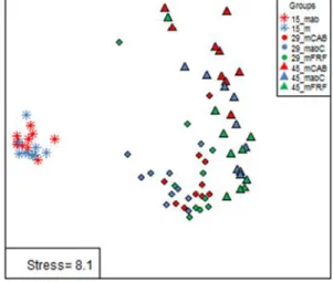
1. Nonmetric Multidimensional Scaling (nMDS)

We apply the function "metaMDS" of the package "vegan" to perform an nMDS (Figure 2). According to the good rule of thumb, stress=8.1% provides an excellent representation in reduced dimensions. Reading the nMDS plot is straight forward: Each point represents an individual, individuals that are located closer to one another are likely to be more similar than those further apart. We can see that items of age 15 are located closer to items of age 29 and age 45. So individuals of age 15 are more similar to each other than to other individuals. This suggest an effect of diet on the shape of the bacterial community. At age of 15 days young rabbit had only access to mother milk while afterward they had access to solid feed.

Figure 2: Representation of similarities of the bacterial communities cecal rabbits according to their age and treatment

2. Analysis of Similarities (ANOSIM)

Applying the function "anosim" of the R package "vegan", we obtained the following results (Table 1 and Table 2). Between groups 15_m and 15_mab, the R statistic=0,197 which means there exists no difference between both groups. This suggest that administration of antibiotic to mother had no effect on bacterial community structure of the young rabbits they nurse. Between groups 29_mCAB and 15_mab, R statistic=0,999 which means there exists obvious difference. The p-value <0,0001, the difference is significant. We can say that the composition of the bacterial community of these two groups are significantly different.

(21)

19

Table 1: R-statistics of analysis of similarities (ANOSIM) according to ages and treatments Age_lot 15_mab 15_m 29_mCAB 29_mabC 29_mFRF 45_mCAB 45_mabC 15_m 0.197 29_mCAB 0.999 0.999 29_mabC 1.000 1.000 0.053 29_mFRF 0.808 0.784 0.216 0.263 45_mCAB 1.000 1.000 0.835 0.960 0.691 45_mabC 1.000 1.000 0.512 0.727 0.314 0.269 45_mFRF 0.926 0.914 0.536 0.684 0.208 0.549 0.032 Analysis was performed according to age_lot at 8 levels.

Table 2: P-values of analysis of similarities (ANOSIM) according to ages and treatments Age_lot 15_mab 15_m 29_mCAB 29_mabC 29_mFRF 45_mCAB 45_mabC 15_m 0.015 29_mCAB <0.0001 <0.0001 29_mabC <0.0001 <0.0001 0.171 29_mFRF <0.0001 <0.0001 0.004 <0.0001 45_mCAB <0.0001 <0.0001 <0.0001 <0.0001 <0.0001 45_mabC <0.0001 <0.0001 0.001 <0.0001 0.004 0.012 45_mFRF <0.0001 <0.0001 <0.0001 <0.0001 0.002 0.003 0.252

Analysis was performed according to age_lot at 8 levels. 3. Mixed-effects Model

The function "lme" of the R package "nlme" helps us build the mixed-effects model. The reason that we chose the mixed-effects model is the following: Individuals are from different does (rabbits' mother), so that it exists a maternal effect that may affect individuals. Thus there will potentially be a separate intercept for each litter. We take into consideration the random effects of mother and propose the following random intercept model (Finch et al., 2014):

𝑦𝑖𝑗 = 𝛾00+ 𝑈0𝑗 + 𝛽1𝑥𝑖 + 𝜖𝑖𝑗

where 𝑦 is the independent variable OTU; 𝑥 is the dependent variable age_lot. The 𝑖𝑗 subscript refers to the OTU of 𝑖𝑡ℎ individual in the 𝑗𝑡ℎ mother, 𝛾00 represents an average intercept value that

(22)

20 In order to test the null hypothesis that mother has no impact on the OTU of individuals, we apply an analysis of variance (ANOVA) and test whether means are different between the previous model and the following fixed-effects model:

𝑦_𝑖 = 𝛾₀₀+ 𝛽₁𝑥 + 𝜖_𝑖

4. Analysis of variance (ANOVA) and Tuckey HSD test

In the Table 3 we see that the ANOVA P-value for OTU_30 is highly significant and above the threshold of 0.05, indicating the difference between the factor "age_lot" (eight levels). So we can run the Tukey test to see which groups differ. The results show that 15_mab, 15_m belong to the same group, the “a”, 29_mCAB, 29_mabC, 29_mFRF, 45_mAB, 45_mCAB, and 45_mFRF differ from other 2 individuals and belong to the group “b”. For OTU_53, the ANOVA P-value is also significant at the threshold of 0.05, which means that there exists the difference between the "age_lot". The Tuckey result indicates that 29_mCAB, 29_mFRF, 45_mCAB belong to the same group “a”, 15_mab, 15_m belong to the same group, the “b”. 29_mabC, 45_mAB and 45_mFRF are not significantly different from the individuals of 2 groups.

Table 3: Results of ANOVA and Tuckey HSD test

Species p-value 15_mab 15_m 29_mCAB 29_mabC 29_mFRF 45_mAB 45_mCAB 45_mFRF

OTU_30 <0.0001 5.614 4.635 0.356 0.841 0.245 1.447 0.65 0.163 a a b b b b b b OTU_53 <0.0001 0.001 0 0.722 0.275 0.875 0.033 0.431 0.178 b b a ab a ab a ab OTU_21 <0.0001 0 0 0.164 0.144 0.014 1.121 0.416 0.027 a ab c bc c c c c OTU_4 <0.0001 10.954 7.285 0.13 0.445 0.236 0.218 0.067 0.274 ab b ab a b ab ab ab OTU_39 <0.0001 0.002 0 0.013 0.048 0.157 0.427 0.136 0.633 a a a a a a a a … … … … …

Within the row: means with different letters are different at P<0.05.

5. Dimension reductions

Since sizes of cecal bacterial community matrix and genes expressions matrix are too big, we want to reduce its dimensions regarding to capacity of analysis. We use the quantile approach to reduce dimensions of genes expressions matrix. In order to optimize the rCCA results, we choose quantile equals to 7. The reduced genes expressions matrix contains 44 individuals and 551 variables. For genes expressions matrix, reduction method is proposed in differential study of differentials genes

(23)

21 expressions (Jacquier et al. 2015). The extracted genes expressions matrix contains 44 individuals and 1781 variables.

6. Regularized canonical correlation analysis (rCCA)

We want to determine how our three matrix relate to each other, so we run rCCA to examine relationships between pairwise matrix and we run RGCCA to determine associations between three blocks of variables.

a) Fermentative parameter dataset and OTU dataset

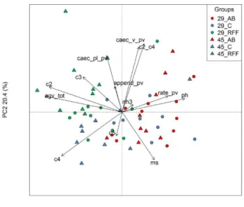
Before applying rCCA, we use PCA as a preliminary step to determine the biggest sources of the variation in the fermentative parameter dataset. This result is represented in Figure 3.

Figure 3: PCA representation of the variability of the fermentation parameters and organ weights

(Caec_pl_pv , cac_v_pv , append_pv , rate_pv : Weight on the live weight of the full cecum , empty, the vermiform appendix , and respectivement speed; ms , NH3, ph agv_tot , c2, c3 , c4 , c2_c4 : dry matter content ammonia , the volatile fatty acids, acetate, propionate, butyrate and acetate butyrate report on cecal content ) .

rCCA is performed on the fermentative parameter dataset and the OTU dataset in order to determine how these two matrix relate to each other. The following plot of individuals (Figure 4) allows us to visualize similarities between members. This plot is obtained by projecting the samples into canonical variates. The same class memberships are shown in the same color.

(24)

22

Figure 4: Plot of individuals

In Figure 4, different colors indicate different groups: black represents the “C+AB” group (medicated group), red shows the “C” group (control group) and green for the “FRF” group. Numbers indicate the age of the rabbit: age of 15 days, 29 days and 45 days.

The plot of variables (Figure 5 and 6) shows the relationship between variates and variables. Variables can be represented as vectors; the correlation between two variables can be visualized through the angles between variables (Cao et al., 2014). For example, there exist a strong positive correlation between c3 and c2_c4 and a strong negative correlation between agv_tot and ms.

Figure 5: Plot of variables

In Figure 5, blue triangles represent OTUs and red letters represent fermentative parameters or organ weights.

(25)

23

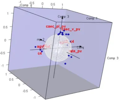
Figure 6: rCCA projection on 3 dimensions of two data sets: OTU and fermentative parameter

For the clustered image map (Figure 7), the green and red colors indicate negative and positive correlations respectively, whereas yellow indicates small correlation values. For example, c3 and Bacteriodacea;Incertae_Sedis OTU_198 are strongly, positively correlated. Rate_pv and Ruminococcaceae;uncultured OTU_10 are strongly, negatively correlated.

Figure 7: Representation of correlations between bacterial species and fermentation parameters & organ weights

(26)

24 The values present the similarity value between the variables of the two data sets. X coordinate indicates fermentative parameters and Y coordinate indicates OTUs and their taxonomic affiliate. For example, Bacteriodacea;Incertae_Sedis OTU_198 indicates that OUT_198 was affiliated to genus of the Bacteriodacea;Incertae_Sedis family.

b) Genes expressions dataset and fermentative parameter dataset

As previous analysis, we run a PCA as preliminary step to determine the biggest sources of variation in the genes expressions dataset. From the 3d plot of individuals (Figure 8), we can see that the third principal component is represented only by individual VJ89 so we extract it from original data and get the new 3d plot of individuals (Figure 9). rCCA is performed on the fermentative parameter dataset (contains 57 individuals and 13 variables of the fermentation parameters and organ weights) and the genes expressions dataset (47 individuals and 16928 variables) in order to determine how these two matrix relate to each other.

Figure 8: 3dPlot of individuals of genes expressions with VJ89

Figure 9: 3dPlot of individuals of genes expressions without VJ89

In Figure 9, different colors indicate different groups: pink represents the 29 days“C+AB” group (medicated group), red represents the 45 days “C+AB” group, light blue shows the 29 days “C” group (control group), dark blue shows the 45 days “C” group, light green for the 29 days “FRF” group and green for the 45 days “FRF” group.

For the clustered image map (Figure 10), the green and red colors indicate negative and positive correlations respectively, whereas yellow indicates small correlation values. For example, PIK3R1 and Bacteriodacea;Bacteroides OTU_1 are strongly, positively correlated. TSRT and S247;NA OUT_406 are strongly, negatively correlated.

(27)

25

Figure 10: Representation of correlations between organ weights and genes expressions & fermentation parameters

X coordinate indicates OTUs and their taxonomic affiliate and Y coordinate indicates fermentative parameters. For example, Bacteriodacea;Bacteroides OTU_1 indicates that OUT_1 was affiliated to genus of the Bacteriodacea; Bacteroides family.

c) Genes expressions dataset and OTU dataset

rCCA is performed on the Genes expressions dataset and OTU dataset in order to determine how these two matrix relate to each other. The following plot of individuals (Figure 11) allows us to visualize similarities between members. This plot is obtained by projecting the samples into canonical variates. The same class memberships are shown in the same color.

For the clustered image map (Figure 12), the green and red colors indicate negative and positive correlations respectively, whereas yellow indicates small correlation values

(28)

26

Figure11: Plot of individuals

Figure12: Representation of correlations between organ weights and genes expressions & bacterial species

d) RGCCA for multigroup data analysis

We use the function rgcca in package RGCCA. The whole data matrix X is partitioned into 3 blocks: 𝑋1 for genes expressions, 𝑋2 for cecal bacterial communities, 𝑋3 for fermentation

parameters. Each column of each group is centered and normalized. We want to determine how genes and cecal bacterial communities influence each other and the impact of fermentations on genes and

cecal bacterial. The correlation matrix is proposed as the following: (

0 1 0 1 0 0 1 1 0

(29)

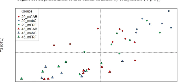
27 have been constructed for each block. The graphical display of the individuals obtained by crossing the two first two components of the superblock ( 𝑌1, 𝑌2) is shown in Figure 13. We can observe that

the bottom part of the graph concentrates individuals of 45 days while the upper part concentrates individuals of 29 days.

Figure 13: Representation of individuals obtained by components ( 𝒀𝟏, 𝒀𝟐)

Figure 14 is built by computing correlations between the first component and the third component. It may be observed individuals from group “C+AB” gather in the left upper part of the graph.

(30)

28 From Figure 15 ( 𝑌₂, 𝑌₃) we observe an obvious distinction of individuals by groups. Individuals of age 29 days from group “C” concentrate in the right upper part while individuals of age 45 days from the same group gather in the left part. Individuals of age 29 days and 45 days from group FRF locate in the right bottom part and left bottom part of the graphical display respectively.

Figure 15: Representation of individuals obtained by components ( 𝒀𝟏, 𝒀𝟑)

Conclusion

Statistical analysis performed on separately the 3 data set and a join analysis for characterizing the composition and the activity of digestive bacterial communities rabbit subjected to three different diets revealed interesting result (effect of diet and age on composition and pinpoint 20 important OTU in the bacterial community). These results will be published in a French national congress.

(31)

29

V. References

Jacquier V., Combes S., Pascal G., Cauquil L., Gabinaud B., Segura M., Bouchez O., Balmisse E.,

Lu S., Estelle J., Oswald I., Rogel-gaillard C., Gidenne T(2015), « Early modulation of the cecal

microbial activity in the young rabbit with rapidly fermentable fiber: Impact on health and growth », Journal of animal science, 92(12):5551-9

Box G. E. P. and Cox D.R. (1964): « An Analysis of Transformations », Journal of the Royal Statistical Society, Vol. 26, No. 2 (1964), pp. 211-252

Zhao L., et al. (2013): « Quantitative Genetic Background of the Host Influences Gut Microbiomes in Chickens », Scientific Reports, 2013; 3:1163

Ramette A. (2007), « Multivariate analyses in microbial ecology », FEMS Microbiology Ecology Vol.62, Iss.2 (November 2007), pp 142–160

Cao K., Conzalez I., Dejean S. (2014), « Multivariate projection methodologies for the exploration of large biological data sets », http://mixomics.org/

Finch W.H., BOLIN J. E., KELLEY K. (2014), « Multilevel modelling using R », CRC Press

Kruskal J.B. (1964), « Multidimensional scaling by optimizing goodness of fit to a nonmetric hypothesis », Psychometrika 29, 1-27

Tenenhaus A., Tenenhaus M. (2014), « Regularized generalized canonical correlation analysis for multiblock or multigroup data analysis », European Journal of Operational Research 238 (2014) 391–403

Kong and Xia Y. (2014), « An adaptive composite quantile approach to dimension reduction », The Annals of Statistics (2014) Vol. 42, No. 4, 1657–1688

(32)

30

VI. Annex

A. List of R packages vegan nlme mixOmics car

B. Definition of OTU (operational taxonomic unit)

The definition given by National Center for Biotechnology Information (NCBI) is: Operational taxonomic unit, species distinction in microbiology. Typically using rRNA and a percent similarity threshold for classifying microbes within the same, or different, OTUs.