Relative merits of different types of observations to constrain galaxy physical parameters

(1)

HAL Id: tel-00834261

https://tel.archives-ouvertes.fr/tel-00834261

Submitted on 14 Jun 2013

HAL is a multi-disciplinary open access

archive for the deposit and dissemination of sci-entific research documents, whether they are pub-lished or not. The documents may come from teaching and research institutions in France or abroad, or from public or private research centers.

L’archive ouverte pluridisciplinaire HAL, est destinée au dépôt et à la diffusion de documents scientifiques de niveau recherche, publiés ou non, émanant des établissements d’enseignement et de recherche français ou étrangers, des laboratoires publics ou privés.

constrain galaxy physical parameters

Camilla Pacifici

To cite this version:

Camilla Pacifici. Relative merits of different types of observations to constrain galaxy physical param-eters. Galactic Astrophysics [astro-ph.GA]. Université Pierre et Marie Curie - Paris VI, 2012. English. �NNT : 2012PA066115�. �tel-00834261�

(2)

THÈSE DE DOCTORAT DE L’UNIVERSITÉ Paris VI Spécialité: Astronomie et Astrophysique Présentée par

Camilla Pacifici

pour obtenir le titre de:

DOCTEUR DE L’UNIVERSITÉ

PIERRE ET MARIE CURIE

Mérites relatifs de différents types

d’observations pour contraindre

les paramètres physiques de

galaxies

Thèse dirigée par Stéphane Charlot

Jury composé de :

Patrick Boissé Président du jury Stéphane Charlot Directeur de thèse Bruno Guiderdoni Rapporteur

Roberto Maiolino Rapporteur Jérémy Blaizot Examinateur Emanuele Daddi Examinateur

(3)

(4)

(5)

(6)

iii

"We are stardust", wrote Joni Mitchell, and this is literally true at the atomic level. Whittet (2003) - Dust in the galactic environment

(7)

(8)

Abstract

The light emitted by galaxies encloses important information about their formation and evolution. The spectral energy distribution of this light across the electromag-netic spectrum contains a myriad of details about the stellar, nebular and dust com-ponents of galaxies. To interpret these features in terms of constraints on physical parameters, we require sophisticated models of the spectral emission from galaxies. In this thesis, we present a new approach to assess the relative merits of different types of observations to constrain galaxy physical parameters, such as stellar mass, star formation rate, metal enrichment of the gas and optical depth of the dust. To this goal, we build a comprehensive library of galaxy spectral energy distributions by combining the semi-analytic post-treatment of a large cosmological simulation with state-of-the-art models of the stellar and nebular emission and attenuation by dust. Using this library, we build a set of galaxy pseudo-observations by convolving spectral energy distributions of models with known parameters with different in-strument response functions and then adding artificial noise. This approach allows us to quantify the accuracy and uncertainty to which physical parameters can be extracted from different types of observations. A main novelty of our approach is the ability to interpret simultaneously the stellar and nebular emission from galaxies, even at low spectral resolution.

We present three applications of our approach to the interpretation of spec-troscopic and photometric observations of galaxies at different redshifts. We first analyze the medium-resolution, rest-frame optical spectra of a sample of ∼ 13, 000 nearby star-forming galaxies extracted from the Sloan Digital Sky Survey (SDSS). We show that the analysis of the combined stellar and nebular emission of these galaxies using our approach provides likelihood distributions of stellar mass, gas-phase oxygen abundance, total effective optical depth of the dust and specific star formation rate similar to those obtained in previous separate analyses of the stellar and nebular emission at the original (twice higher) SDSS spectral resolution.

Then, we apply our approach to the analysis of combined photometric and spec-troscopic observations of a sample of galaxies at redshifts between 1 and 3. We ex-plore the relative advantages and the complementarity of ultraviolet-optical-infrared photometry and rest-frame ultraviolet and optical spectroscopy to constrain the physical parameters of these galaxies.

Finally, we use our approach to simulate observations of primeval galaxies with the NIRSpec instrument onboard the future James Webb Space Telescope (JWST). We achieve this by feeding model spectra, calibrated using the deepest available photometric observations, into a preliminary version of the NIRSpec instrument performance simulator. We explore with particular attention the ability to interpret the rest-frame ultraviolet properties of primeval galaxies using our approach. This work will be valuable to quantify the improvements that low- and medium-resolution spectroscopy with JWST/NIRSpec will bring compared to currently available

(13)

pho-tometric datasets when exploring the physical parameters of the very ﬁrst galaxies that formed in the early Universe.

The approach developed in this thesis can be used to extract valuable information from any kind of galaxy observation across the wavelength range covered by spectral evolution models as well as to plan for future galaxy observations.

(14)

Résumé

La lumière émise par les galaxies contient des informations importantes sur leur formation et leur évolution. La distribution spectrale d’énergie de cette lumière à travers le spectre électromagnétique contient elle même une myriade de détails sur les composants stellaire, nébulaire et de la poussière des galaxies. Pour interpréter ces caractéristiques en termes de contraintes sur certains paramètres physiques, nous avons besoin de modèles sophistiqués de l’émission spectrale des galaxies.

Dans cette thèse, nous présentons une nouvelle approche pour évaluer les mérites relatifs des différents types d’observations pour contraindre certains paramètres physiques des galaxies tels que la masse stellaire, le taux de formation stellaire, l’enrichissement en métaux du gaz et la profondeur optique de la poussière. Pour cet objectif, nous construisons une bibliothèque complète de distributions spec-trales d’énergie des galaxies en combinant un traitement semi-analytique d’une grande simulation cosmologique avec des modèles de pointe de l’émission stellaire et nébulaire et de l’atténuation par la poussière. En utilisant cette bibliothèque, nous construisons un ensemble de pseudo-observations de galaxies par convolu-tion des distribuconvolu-tions spectrales d’énergie des modèles, dont nous connaissons les paramètres physiques, avec des fonctions de réponse de différents instruments, puis en ajoutant du bruit artificiel. Cette approche nous permet de quantifier la préci-sion et l’incertitude à la quelle les paramètres physiques peuvent être extraites de différents types d’observations. Une principale nouveauté de notre approche est la capacité d’interpréter simultanément l’émission stellaire et nébulaire des galaxies, même à faible résolution spectrale.

Nous présentons trois applications de notre approche pour l’interprétation d’observations spectroscopiques et photométriques de galaxies à diﬀérents redshifts. Nous analysons d’abord des spectres optiques (rest-frame) en résolution moyenne d’un échantillon de ∼ 13,000 galaxies à proximité extraites du Sloan Digital Sky Survey (SDSS). Nous montrons que l’analyse de la composante stellaire combinée à la composante nébulaire de ces galaxies en utilisant notre approche fournit des dis-tributions de probabilité de la masse stellaire, de l’abondance de l’oxygène en phase gazeuse, de la profondeur optique de la poussière et du taux spéciﬁque de formation stellaire similaires à ceux obtenus dans des analyses séparées des composantes stel-laire et nébustel-laire à la résolution spectrale originale du SDSS, qui est deux fois plus élevée.

Ensuite, nous appliquons notre approche à l’analyse combiné des observations photométriques et spectroscopiques d’un échantillon de galaxies à redshift entre 1 et 3. Nous explorons les avantages relatifs et la complémentarité de la photométrie ultraviolet, optique et infrarouge et de la spectroscopie ultraviolet et optique pour contraindre les paramètres physiques de ces galaxies.

Enﬁn, nous utilisons notre approche pour simuler des observations de galax-ies primitives avec l’instrument NIRSpec à bord du future télescope spatial James

(15)

Webb (JWST). Nous réaliserons cela en utilisant des spectres, extraits de notre bibliothèque et calibré à l’aide des plus profondes observations photométriques disponibles, dans une version préliminaire du simulateur des performances de l’instrument NIRSpec. Nous explorons en particulier la capacité à interpréter les propriétés des longueurs d’onde ultraviolets (reste-frame) de galaxies primitives en utilisant notre approche. Ce travail sera très utile pour quantiﬁer les améliora-tions que la spectroscopie de faible et moyenne résolution avec JWST / NIRSpec apporteront par rapport à des données photométriques actuellement disponibles en explorant les paramètres physiques des toutes premières galaxies qui se sont formées dans l’Univers primordial.

L’approche développée dans cette thèse peut être utilisée pour extraire des in-formations précieuses à partir de n’importe quel type d’observation de galaxies sur toute la gamme de longueurs d’onde couvertes par les modèles d’évolution spectrale ainsi que pour planiﬁer de futures observations de galaxies.

(16)

List of Figures

1.1 A broad view of the most important telescopes and the wavelength ranges they cover. The atmospheric absorption coeﬃcient is also shown. 3 1.2 Photometric images of the galaxy NGC1512 in diﬀerent bands.

Clock-wise from left to right: far ultraviolet (∼ 2000Å), near ultraviolet (∼ 3000Å), optical (∼ 5000Å), Hα emission (6563Å), near infrared (∼ 1µm), mid infrared (∼ 10µm) and far infrared (∼ 100µm). Credit: NASA. . . 4 1.3 Panel (a): spectral energy distribution of a galaxy at optical

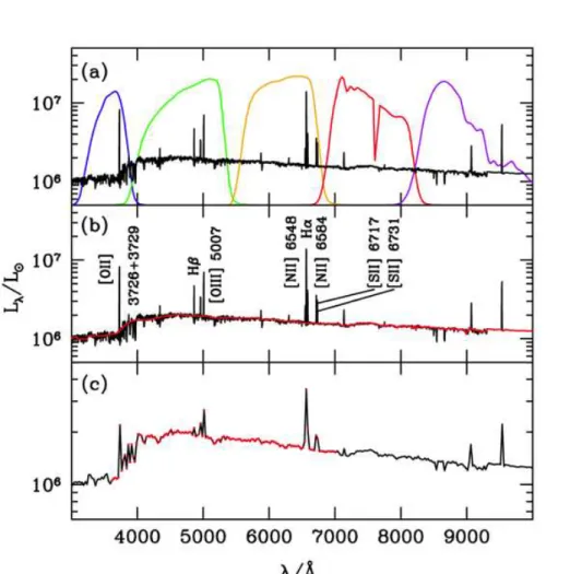
wave-lengths (black line) overlaid are the ﬁve ﬁlter response functions of the SDSS. Panel (b): same spectral energy distribution as in panel (a) (black line), with the strongest emission lines labeled; the red line shows the stellar continuum underneath the lines. Panel (c): the same spectral energy distribution as in panel (a), computed at a 10-times lower resolution; red points mark the binning. Note that the ordinate scale in panel (c) is enlarged. . . 6 1.4 Flowchart of the general idea behind this thesis. . . 9 2.1 Fig. 9 from Madau et al. [1996], showing on the left the Universal

metal ejection density, ˙ρZ, and on the right the total star formation

rate density, ˙ρ∗, as a function of redshift. Triangle: Gallego et al.

[1995]. Filled dots: Lilly et al. [1996]. Filled squares: lower limits from Hubble Deep Field images. . . 13 2.2 Fig. 5 from Cucciati et al. [2011], showing the total dust-corrected

UV-derived star formation rate density as a function of redshift from the VVDS sample (red ﬁlled circles). The black dashed line is the star formation rate density as a function of z implied from the stellar mass density in Ilbert et al. [2010]. Other data sets are overplotted and labeled on the ﬁgure. All data have been converted into a star formation rate density with the scaling relation from Madau et al. [1998]. . . 13 2.3 Idealized star formation histories (panels a, b, c) and the relative

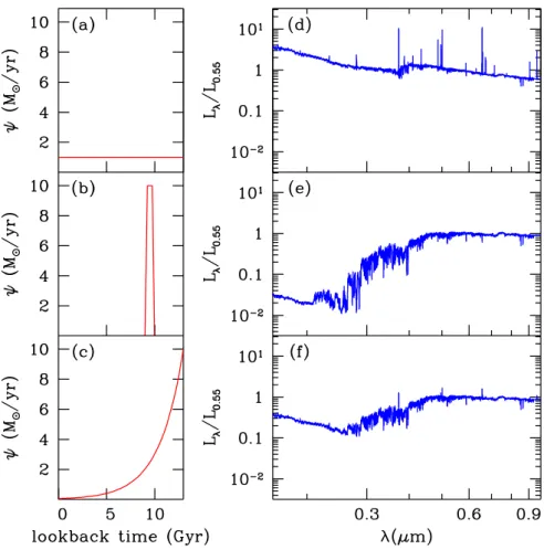
spectral energy distributions (panels d, e, f). The model spectral en-ergy distributions are computed using the latest version of Bruzual and Charlot [2003] at ﬁxed solar metallicity, with a Chabrier initial mass function [Chabrier, 2003]. Emission lines are computed con-sistently following the prescription by Charlot and Longhetti [2001]. The attenuation by dust is neglected in these examples. . . 15

(17)

2.4 Fig. 10 from Kauﬀmann et al. [2003a]. Observed g − r versus r − i colors of a representative sample of SDSS galaxies (black points) for 2 particular redshifts (0.11 and 0.03). Blue points represent the model grid, computed applying Bruzual and Charlot [2003] models to ex-ponentially declining star formation histories, with random super-imposed burst of star formation. In the left panels, data are not corrected for dust attenuation, while in the right panels, data are corrected with an attenuation law of the form τλ ∝ λ−0.7. The red

arrow shows the predicted reddening vector. . . 16 2.5 Fig. 2 from De Lucia and Blaizot [2007]. The merger tree of a

dark matter halo of ∼ 9 × 1014 _M

⊙. The area of the symbols scales

with the mass. Circles represent haloes that are part of the friends-of-friends group, while triangles show haloes that have not joined yet the friends-of-friends group. The halo which contains the main branch is marked in green. The trees on the right-hand side, which are not linked to the main halo, correspond to the other substructures identiﬁed in the friends-of-friends group at z = 0. . . 19 2.6 Stellar initial mass faction normalized to solar units. Salpeter [1955],

blue line. Miller and Scalo [1979], magenta line. Kroupa [2001], green line. Chabrier [2003], dashed line. . . 23 2.7 The Hertzsprung-Russell diagram (H-R) shows the evolutionary

stages of stars in terms of their luminosity and temperature. Differ-ent evolutionary paths for stars of differDiffer-ent initial masses are plotted in different colors. The zero-age main sequence is shown as a black solid line. The labels indicate the main stages of the evolution. . . . 25 2.8 Fig. 2 and 3 from Heger et al. [2003]. Stellar mass at the time of

final explosion or remnant formation (blue line), remnant mass (red line) and metals released in the interstellar medium (green fill and hatching) as a function of initial mass of the stars for solar metallicity (top panel) and for zero metallicity (bottom panel). . . 28 2.9 Top panel: isochrones from Bertelli et al. for different ages at solar

metallicity, solid lines; isochrones from other models in the Padova database at solar metallicity, dashed lines. Bottom panel: zoom of the yellow region in the top panel, showing isochrones (ages between 0.06 and 16 Gyr) form Marigo et al. [2008] (Fig. 1) for pre-TP-AGB phase in green, and O-rich and C-rich conﬁgurations of the TP-AGB phase respectively in blue and red. . . 32 2.10 Representation of the diﬀerent phases of the interstellar medium in

terms of temperature and density. . . 34 2.11 A schematic representation of an H ii region. The ionizing

source is shown in the center. The region occupied by the ion-ized hydrogen (Stromgren sphere) is shown in blue. The region ﬁlled by the neutral hydrogen is shown in pink. (Figure from http://www.astro.cornell.edu/academics/) . . . 36

(18)

List of Figures xv 2.12 Frequency variation of the free-bound continuous-emission coeﬃcient

γν(T ) for hydrogen (black solid line) and for helium (black thin solid

line). Frequency variation of the two-photon-process coeﬃcient (grey solid line). All lines correspond to a low-density regime at T = 10, 000 K. Figure from Osterbrock and Ferland [2006]. . . 37

2.13 Typical spectrum of an H ii region with the strongest lines labeled. (htp://frigg.physastro.mnsu.edu) . . . 38

2.14 Extinction curves (Aλ/AV) as a function of wavelength in the

ultra-violet and optical rest-frame ranges. The red line shows the aver-age extinction curve of the Milky Way as in Cardelli et al. [1989] (RV = 3.1). The short-dashed line shows the extinction curve of the

Small Magellanic Cloud bar, while the long-dashed line shows the average extinction curve of the Large Magellanic Cloud, both as in Gordon et al. [2003]. The blue line represents the extinction curve by Calzetti et al. [2000] and the green line shows a curve of the form λ−0.7 _{normalized at 5500Å. . . 45}

2.15 Trasmission coefficient in the intergalactic medium at three different redshifts: z = 3.0 (red line), z = 4.5 (green line), z = 6.0 (blue line). Dotted lines represent the Lyman limit (912Å) at the three different redshifts. . . 50

3.1 Example of galaxy star formation and chemical enrichment histories inferred from the semi-analytic post-treatment of the Millennium cos-mological simulation: (a) star formation rate, ψ, and (b) interstellar metallicity, Z, plotted as a function of look-back time, for a galaxy with a present-day stellar mass of 1.5 × 1010_M

⊙. The vertical dashed

line marks the evolutionary stage at which the galaxy is looked at in Fig. 3.3 (corresponding to a galaxy age of 8.4 Gyr). . . 56

(19)

3.2 Emission-line luminosities of galaxies computed using the models de-scribed in Section 3.2.2.2 (lines), compared with high-quality obser-vations of a sample of 28,075 star-forming galaxies from the SDSS DR7 (black dots). The models assume constant star formation over the past 10 Myr. The data are corrected for attenuation by dust as described in Brinchmann et al. [2004]. (a) L([O iii]λ5007)/L(Hβ) versus L([N ii]λ6584)/L(Hα). (b) L([O iii]λ5007)/L(Hβ) versus L([S ii]λλ6716, 6731)/L(Hα). (c) L([O iii]λ5007)/L(Hβ) versus L([N ii]λ6584)/L([O ii]λ3727). (d) L([O iii]λ5007)/L(Hβ) versus L([O ii]λ3727)/L([O iii]λ5007). In each panel, lines of diﬀerent colours refer to models with diﬀerent zero-age ionization parame-ter log U0 (cyan: −1.5; red: −2.0; green: −2.5; magenta: −3.0;

blue: −3.5). At ﬁxed log U0, the lower dashed line corresponds to

models with dust-to-metal ratio ξd = 0.1, the solid line to models

with ξd = 0.3 and the upper dashed line to models with ξd = 0.5.

Along each line, dots mark the positions of models with diﬀerent gas metallicity Z (0.10, 0.20, 0.50, 0.75, 1.00, 1.50, 2.00 and 3.00 times Z⊙, from left to right; only low-metallicity models are considered for

log U0 = −1.5). In (a), the gray long-short-dashed line shows the

Kauﬀmann et al. [2003b] criterion to separate star-forming galaxies from AGNs. . . 61

3.3 Spectral energy distribution of the same model galaxy as in Fig. 3.1 at the age of 8.4 Gyr, computed using the models described in Sec-tions 3.2.1 and 3.2.2. (a) At a spectral resolution of 5 Å FWHM (R = 1000 at 5000 Å). The black portion of the spectrum (λ=3600– 7400 Å) is that used to retrieve galaxy physical parameters at this resolution. (b) Same as in (a), but at a spectral resolution of 50 Å FWHM (R = 100 at 5000 Å). (c) Same as in (a), but convolved with the SDSS ugriz ﬁlter response functions (shown at the bottom). The model galaxy has fSFH= 0.3 and current parameters (resampled

us-ing the distributions in Table 3.1) ψS = 0.08 Gyr−1, Z = 0.4Z⊙,

log U0 = −2.8, ξd = 0.3, ˆτV = 1.0, µ = 0.6 and n = 0.7. In (a) and

(20)

List of Figures xvii 3.4 Prior distributions of selected physical parameters of the 5

mil-lion galaxies in the spectral library generated in Section 3.2.3: (a) observer-frame absolute r-band stellar mass-to-light ratio, M∗/Lr; (b)

fraction of current stellar mass formed during the last 2.5 Gyr, fSFH;

(c) speciﬁc star formation rate, ψS; (d) gas-phase oxygen abundance,

12 + log (O/H); (e) total eﬀective V -band absorption optical depth of the dust, ˆτV; (f) fraction of ˆτV arising from dust in the ambient ISM,

µ. In each panel, the shaded histogram shows the distribution for all galaxies, while the solid histogram shows the contribution by star-forming galaxies alone. Non-star-star-forming galaxies are oﬀ scale (at log ψS = −∞) in panel (c) and do not contribute to the distributions

of interstellar parameters in panels (d)–(f). . . 69 3.5 Probability density functions of the same physical parameters as in

Fig. 3.4 retrieved, using the Bayesian approach described in Sec-tion 3.2.4, from the pseudo-galaxy spectrum shown at the top. The spectrum was obtained by adding artiﬁcial noise with S/N = 20 to the R = 100 model spectrum of Fig. 3.3b. In each panel, the black tri-angle indicates the true value of the parameter of the pseudo-galaxy, the solid line the best estimate (50th percentile of the retrieved like-lihood distribution) and the dashed lines the associated 68-percent conﬁdence interval (16th and 84th percentiles). . . 70 3.6 Average probability density functions of the same 6 physical

param-eters as in Fig. 3.4 retrieved, using the Bayesian approach described in Section 3.2.4, from 5-band ugriz photometry with S/N = 30 of a sample of 10,000 pseudo-galaxies (standard case). Each panel corre-sponds to a diﬀerent parameter [from left to right: M∗/Lr, fSFH, ψS,

12 + log (O/H), ˆτV and µ]. In each case, average probability density

functions in 50 narrow bins of true parameter value were obtained by coadding and then renormalizing the probability density functions retrieved for the 10,000 pseudo-galaxies (see Section 3.3.1.1 for de-tail). Grey levels locate the 2.5th, 12th, 16th, 22nd, 30th, 40th, 60th, 70th, 78th, 84th, 88th and 97.5th percentiles of the average likelihood distribution in each bin. The solid line locates the associated median (best estimate) and the 2 dashed lines the 16th and 84th percentiles (68-percent conﬁdence interval). For reference, 3 dotted lines indi-cate the identity relation and deviations by a factor of 2 (±0.3 dex) between the retrieved and true parameter values. . . 72 3.7 (a) g − i colour plotted against u − g colour for a subset of 50,000

models from the galaxy spectral library assembled in Section 3.2.3. The models are colour-coded according to speciﬁc star formation rate, as indicated. (b) Same as (a), but without including the contribution by nebular emission to broadband ﬂuxes. . . 74

(21)

3.8 Same as Fig. 3.6, but for 3 distinct alternatives to the standard case: (top row) adopting a signal-to-noise ratio S/N = 10 instead of 30; (middle row) using constraints from only the ugr photometric bands instead of ugriz; and (bottom row) not including nebular emission in the model library used to analyze the sample of 10,000 pseudo-galaxies. In all cases, the improvement factor Iσ and the gain in

accuracy ∆ (equations 3.3.13–3.3.14) are shown as a function of true parameter value at the bottom of each panel to quantify diﬀerences in the retrieved likelihood distributions relative to the standard case of Fig. 3.6. . . 77 3.9 Prior distributions of the same physical parameters as in Fig. 3.4

for the 5 million galaxies at redshifts between 0 and 1 in the spec-tral library assembled in Section 3.3.1.2. In each panel, the shaded histogram shows the distribution for all galaxies, while the solid his-togram shows the contribution by star-forming galaxies alone. Non-star-forming galaxies are oﬀ scale (at log ψS = −∞) in panel (c) and

do not contribute to the distributions of interstellar parameters in panels (d)–(f). . . 78 3.10 (a) Distribution of the diﬀerence between the retrieved best estimate

(i.e. median) and true value of zobs, in units of 1 + zobs, for a sample

of 10,000 pseudo-galaxies at redshifts between 0 and 1 observed in the ugriz photometric bands. The shaded and solid histograms show the distributions obtained for S/N = 30 and S/N = 10, respectively. For reference, a dashed line indicates the σ = 0.03 Gaussian accuracy quoted by Ilbert et al. [2006], who analyzed CFHTLS (S/N & 30) u∗_g′_r′_i′_z′ photometry of about 3000 galaxies with spectroscopic

red-shifts between 0.2 and 1.5. (b) Detail of the average retrieved proba-bility density function plotted against zobs, for S/N = 30. The lines

and shading have the same meaning as in Fig. 3.6. (c) Same as (b), but for S/N = 10. . . 80 3.11 Average probability density functions of the same 6 physical

parame-ters as in Fig. 3.9 retrieved, using the Bayesian approach described in Section 3.2.4, from 5-band ugriz photometry with S/N = 30 of sam-ples of 10,000 pseudo-galaxies at random redshifts: (top row) drawn in the redshift range 0.2 < zobs < 0.4; and (bottom row) drawn in

the redshift range 0.6 < zobs < 0.8. In each case, the redshift zobs

of a galaxy is assumed not to be known a priori, and the probability density functions are computed using models at all redshifts between 0 and 1 in the spectral library assembled in Section 3.3.1.2. In all panels, the lines and shading have the same meaning as in Fig. 3.6. . 81

(22)

List of Figures xix 3.12 Average probability density functions of the speciﬁc star formation

rate, ψS, gas-phase oxygen abundance, 12 + log (O/H), and dust

at-tenuation optical depth in stellar birth clouds, (1 − µ)ˆτV, retrieved,

using the Bayesian approach described in Section 3.2.4, from the equivalent widths of optical emission lines in a sample of 10,000 star-forming pseudo-galaxies. The sample was extracted from the library of galaxy spectral energy distributions assembled in Section 3.2.3, assuming a median signal-to-noise ratio per pixel S/N = 20 and re-quiring 3σ measurements of all line equivalent widths. (Top row) using the equivalent widths of [O ii]λ3727; Hβ; [O iii]λλ4959, 5007; [N ii]λ6548+Hα+[N ii]λ6584; and [S ii]λλ6716, 6731 at a spectral res-olution of 50 Å FWHM (R = 100 at λ = 5000 Å). (Bottom row) using the equivalent widths of [O ii]λ3727; Hβ; [O iii]λ4959; [O iii]λ5007; [N ii]λ6548; Hα; [N ii]λ6584; [S ii]λ6716 and [S ii]λ6731 at a spectral resolution of 5 Å FWHM (R = 1000 at λ = 5000 Å). In all panels, the lines and shading have the same meaning as in Fig. 3.6. . . 84 3.13 Average probability density functions of the same 6 physical

param-eters as in Fig. 3.4 retrieved, using the Bayesian approach described in Section 3.2.4, from low-resolution optical spectra of a sample of 10,000 pseudo-galaxies. The spectra cover the wavelength range from λ = 3600 to 7400 Å at the resolution of 50 Å FWHM (R = 100 at λ = 5000 Å) with median signal-to-noise ratio per pixel S/N = 20. (Top row) for a sample of 10,000 pseudo-galaxies extracted randomly from the spectral library assembled in Section 3.2.3. The improve-ment factor Iσ and the gain in accuracy ∆ (equations 3.3.13–3.3.14)

are shown as a function of true parameter value at the bottom of each panel to quantify diﬀerences in the retrieved likelihood distributions relative to the standard case of Fig. 3.6. (Bottom row) for a sample of 10,000 star-forming pseudo-galaxies extracted from the same spectral library, with the requirement that the net Hα+[N ii] emission equiv-alent width be greater than 5 Å. In all panels, the lines and shading have the same meaning as in Fig. 3.6. . . 86 3.14 Same as Fig. 3.13, but: (top row) adopting a median signal-to-noise

ratio per pixel S/N = 5 instead of 20; (bottom row) not including nebular emission in the model library used to analyze the sample of 10,000 pseudo-galaxies. In both cases, the improvement factor Iσ

and the gain in accuracy ∆ (equations 3.3.13–3.3.14) are shown as a function of true parameter value at the bottom of each panel to quantify diﬀerences in the retrieved likelihood distributions relative to the standard case of Fig. 3.6. . . 87

(23)

3.15 Average probability density functions of the same 6 physical param-eters as in Fig. 3.4 retrieved, using the Bayesian approach described in Section 3.2.4, from medium-resolution optical spectra of a sample of 10,000 pseudo-galaxies. The spectra cover the wavelength range from λ = 3600 to 7400 Å at the resolution of 5 Å FWHM (R = 1000 at λ = 5000 Å) with median signal-to-noise ratio per pixel S/N = 20. (Top row) for a sample of 10,000 pseudo-galaxies extracted randomly from the spectral library assembled in Section 3.2.3. The improve-ment factor Iσ and the gain in accuracy ∆ (equations 3.3.13–3.3.14)

are shown as a function of true parameter value at the bottom of each panel to quantify diﬀerences in the retrieved likelihood distributions relative to the standard case of Fig. 3.6. (Bottom row) for a sample of 10,000 star-forming pseudo-galaxies extracted from the same spec-tral library, with the requirement that the net Hα emission equivalent width be greater than 5 Å. In all panels, the lines and shading have the same meaning as in Fig. 3.6. . . 90

3.16 Estimates of physical parameters retrieved from the spectra of 12,660 SDSS star-forming galaxies (degraded to a resolution of 5 Å FWHM) using the Bayesian approach described in Section 3.2.4 plotted against estimates of the same parameters from diﬀerent sources, as indi-cated. (a) Stellar mass, M⋆. (b) Gas-phase oxygen abundance,

12 + log (O/H). (c) Total V -band attenuation optical depth of the dust, ˆτV. (d) Speciﬁc star formation rate, ψS. In each panel, the

like-lihood distributions from previous studies were reconstructed from the published 16th, 50th and 84th percentiles and combined with the likelihood distributions obtained in this work to generate 2D proba-bility density functions. The contours depict the normalized co-added 2D probability density function including all 12,660 galaxies in the sample (on a linear scale 25 levels, the outer edge of the lightest grey level corresponding to the 96th percentile of the 2D distribution). The solid line is the identity relation. . . 93

(24)

List of Figures xxi 3.17 Two-dimensional probability density functions of the fraction of the

current stellar mass formed during the last 2.5 Gyr, fSFH, versus

stel-lar mass, M⋆, speciﬁc star formation rate, ψS, gas-phase oxygen

abun-dance, 12 + log (O/H), total V -band attenuation optical depth of the dust, ˆτV, and fraction of ˆτV arising from dust in the ambient ISM,

µ. All parameters were retrieved from the spectra of the same 12,660 SDSS star-forming galaxies as in Fig. 3.16 (degraded to a resolution of 5 Å FWHM) using the Bayesian approach described in Section 3.2.4. In each panel, the contours depict the normalized co-added 2D prob-ability density function including all 12,660 galaxies in the sample (on a linear scale of 25 levels, the outer edge of the lightest grey level corresponding to the 96th percentile of the 2D distribution). All physical quantities pertain to the regions of galaxies probed by the 3-arcsec-diameter SDSS ﬁbers. . . 95

3.18 Prior distributions of the same physical parameters as in Fig. 3.4 for the 5 million galaxies in the spectral library generated in Section 3.4.2. These distributions are those arising, at the mean redshift z = 0.07 of the SDSS sample of Section 3.4.1, from the original semi-analytic post-treatment of the Millennium cosmological simulation of Springel et al. [2005] by De Lucia and Blaizot [2007, see text for detail]. In each panel, the shaded and thin solid histograms have the same meaning as in Fig. 3.4. In panels (a), (c), (d) and (e), the thick solid his-tograms show the distributions of the best estimates of M∗/Lr, ψS,

12 + log (O/H) and ˆτV from Gallazzi et al. [2005], Brinchmann et al.

[2004] and Tremonti et al. [2004] for the same sample of 12,660 SDSS star-forming galaxies as in Fig. 3.16. . . 97

3.19 Same as Fig. 3.16, but using the prior distributions in Fig 3.18 instead of those in Fig. 3.4 to retrieve the probability density functions of M⋆,

12 + log (O/H), ˆτV and ψS for the 12,660 SDSS star-forming galaxies

in the sample. . . 98

4.1 Galaxy #1705. The G141 spectrum (red dotted line), the part of the spectrum used in the analysis (1.1 ≤ λ ≤ 1.6µm, blue solid line), J-band eﬀective wavelength (magenta dashed line) and square band of 0.1 µm width (magenta solid line). . . 106

(25)

4.2 Top panel: MAGPHYS ﬁt (zgrism = 2.21 is the input redshift) to

the FIREWORKS photometry (red dots) of galaxy #1799; the black spectrum is the best-fit model and the blue spectrum is the pure stellar spectrum (i.e. unattenuated by dust) corresponding to this best-fit model. Middle panel: zoom of the observed-frame wavelength range from the ultraviolet to the near-infrared; FIREWORKS pho-tometry (red dots), MAGPHYS best-fit model spectrum (black line), 3D-HST spectrum (green line) with error bars (grey). Bottom pan-els: histograms showing the likelihood distributions of the fraction of total dust luminosity contributed by the diffuse ISM, fµ, the total

op-tical depth seen by young stars in birth clouds, τV, the optical depth

seen by stars in the diﬀuse ISM, µτV, the star formation rate, ψ, the

speciﬁc star formation rate, ψS, the stellar mass, M∗, and total dust

luminosity, Ltot

d . . . 109

4.3 Prior distributions of selected physical parameters of the 2,500,000 galaxies in the spectral library: (a) rest-frame absolute V-band stellar mass-to-light ratio, M∗/L₅₅; (b) fraction of the current galaxy stellar

mass formed during the last Gyr, fSFH; (c) speciﬁc star formation

rate, ψS; (d) gas-phase oxygen abundance, 12 + log (O/H); (e) total

eﬀective V-band absorption optical depth of the dust, ˆτV; (f) fraction

of ˆτV arising from dust in the ambient ISM, µ. In each panel, the

shaded histogram shows the distribution for all galaxies, while the solid histogram shows the contribution by star-forming galaxies alone. Non-star-forming galaxies are oﬀ scale (at log(ψS) = ∞) in panel (c)

and do not contribute to the distributions of interstellar parameters in panels (d)–(f). . . 110 4.4 Spectral ﬁt of galaxy #1799, using this thesis approach, with no

prior information on redshift. Top panel: the red line is the observed 3D-HST spectrum, and the blue line is the best-fit model spectrum. Medium panel: residuals between the observed and the best-fit model spetra. Bottom panels: histograms showing the likelihood distribu-tions of stellar mass, fraction of stellar mass formed in the last Gyr, specific star formation rate, gas-phase oxygen abundance, total effec-tive optical depth of the dust and redshift. . . 112 4.5 Comparison between the redshift estimates obtained with our

spec-troscopic approach, with the redshift provided in the catalogue

(zgrism). Green dots represent the median estimates when redshift

is treated as a free parameter. Blue crosses represent the median es-timates obtained ﬁtting each galaxy only with models in the range

zgrism± 0.3. Error bars are the 16 and 84 percentiles in the likelihood

distributions. . . 113 4.6 Same as Fig. 4.4. Spectral ﬁt of galaxy #5435, using the approach

(26)

List of Figures xxiii 4.7 Same as Fig. 4.4. Spectral ﬁt of galaxy #5434, using the approach

developed in this thesis. The redshift is constrained to be within 0.3 of zgrism. . . 116

4.8 Left panel: comparison between stellar mass estimates obtained with our spectroscopic approach and the ones obtained with MAGPHYS. Right panel: comparison between speciﬁc star formation rate esti-mates obtained with our spectroscopic approach and the ones ob-tained with MAGPHYS. In both panels, green dots represent the median estimates when redshift is treated as a free parameter. Blue squares represent the median estimates obtained when the redshift is constrained to be within 0.3 of zgrism. Error bars represents the 16th

and 84th percentiles of the likelihood distributions. . . 117 4.9 Top panel: MAGPHYS ﬁt (zgrism = 1.02 is the input redshift) to

the FIREWORKS photometry (red dots) of galaxy #5209; the black spectrum is the best-fit model and the blue spectrum is the pure stellar spectrum (i.e. unattenuated by dust) corresponding to this best-fit model. Middle panel: zoom of the observed-frame wavelength range from the ultraviolet to the near-infrared; FIREWORKS pho-tometry (red dots), MAGPHYS best-fit model spectrum (black line), 3D-HST spectrum (green line) with error bars (grey). Bottom pan-els: histograms showing the likelihood distributions of the fraction of total dust luminosity contributed by the diffuse ISM, fµ, the total

op-tical depth seen by young stars in birth clouds, τV, the optical depth

seen by stars in the diﬀuse ISM, µτV, the star formation rate, ψ, the

speciﬁc star formation rate, ψS, the stellar mass, M∗, and total dust

luminosity, Ltot

d . . . 118

5.1 ACS and NICMOS filters: B in blue, V in magenta, i’ in cyan, z’ in green, J in orange and H in red. In gray, five model galaxies at redshifts 2.15, 3.55, 4.40, 5.78 and 6.72. Flux is expressed in AB mag-nitudes in the observed-range between 0.3 and 2 µm. The increasing effect of the IGM absorption with redshift is visible blueward of the Lyman-α line. . . 123 5.2 Panel a: V −i′_{versus i}′

−z′_{colors. Panel b: i}′

−z′_{versus z}′

−J colors. In both plots, dots represent model galaxies in diﬀerent ranges of redshift: z < 3.5 black, 3.5 < z < 4.5 red, 4.5 < z < 5.5 yellow, 5.5 < z < 6.5 green, 6.5 < z < 7.5 magenta. Grey squares with error bars represent the selected HUDF galaxies. Photometric redshifts from the catalogue by Coe et al. [2006] label a few high-redshift galaxies to identify the outliers in panel (a) and check their position in panel (b). . . 124

(27)

5.3 Prior distributions of selected physical parameters of the 500,000 galaxies in the spectral library: (a) observer-frame absolute H-band stellar mass-to-light ratio, M∗/L_H; (b) redshift, z; (c) speciﬁc star

formation rate, ψS; (d) gas-phase oxygen abundance, 12 + log (O/H);

(e) total eﬀective V-band absorption optical depth of the dust, ˆτV; (f)

fraction of ˆτV arising from dust in the ambient ISM, µ. In each panel,

the shaded histogram shows the distribution for all galaxies, while the solid histogram shows the contribution by star-forming galaxies alone. Non-star-forming galaxies are oﬀ scale (at log(ψS) = ∞) in panel (c)

and do not contribute to the distributions of interstellar parameters in panels (d)–(f). . . 126 5.4 Left panel: rest-frame ultraviolet spectral energy distribution of a

galaxy (z = 3.41) extracted form the model library (black) and the associated power-law best ﬁt (green). The wavelength windows used to perform the ﬁt are highlighted in cyan. Right panel: distribution of the rest-frame ultraviolet slope in the model library for all galaxies (shaded histogram) and for galaxies with negligible 2175Å bump only (solid histogram). . . 127 5.5 ID 5299. Top panel: ACS observed magnitudes (magenta dots),

NICMOS observed magnitudes (red dots), ACS and NICMOS mag-nitudes of the best-fit model galaxy (blue squares), best-fit model spectrum when fitting both ACS and NICMOS magnitudes (black line), best-fit model spectrum when fitting ACS data alone (green line). Middle panel: residuals between best-fit model magnitudes and data (crosses). Bottom panels: probability density functions retrieved for stellar mass, specific star formation rate, gas-phase oxy-gen abundance, total effective optical depth of the dust, rest-frame ultraviolet slope, redshift. In each panel, the shaded histogram was derived by fitting both ACS and NICMOS data, while the solid his-togram was derived using ACS data alone. In the redshift panel, the vertical red line shows the photometric redshift listed in the Coe et al. [2006] catalogue. . . 129 5.6 Example of the multi-object spectrograph (MOS) scene obtained by

placing diﬀerent point-like galaxies ‘behind’ diﬀerent micro-shutters. Light is dispersed using NIRSpec low-resolution prism (R = 100). . . 131 5.7 Zoom of the scene presented in Figure 5.6. In correspondence of every

galaxy, 3 vertically-adjacent micro-shutters are open. In each case, the radiation of the Zodiacal light dominates the background in the upper and lower micro-shutters. The continuum emission from the galaxies and some emission lines (red isolated pixels) can be detected in the central micro-shutter. . . 132

(28)

List of Figures xxv 5.8 Diﬀerences in redshift estimates between our ﬁts and the values

re-ported in Coe et al. [2006] catalogue. Gray squares represent the fits using ACS and NICMOS magnitudes. Black dots represent the fits when ACS magnitudes alone are available. For each measurement, the error bar indicates the sum of the 16th–84th percentile range of the likelihood distribution retrieved from our analysis and the 1-sigma uncertainty in the Coe et al. estimate (≈ 0.3). The red dotted line marks the location of perfect agreement between the two redshift estimates. . . 134 5.9 Estimates of rest-frame ultraviolet slope, β, versus total effective

op-tical depth of the dust, ˆτV. Grey dots: 50,000 random galaxies from

the model library. Red (z < 4) and magenta (z > 4) squares: median estimates ﬁtting both ACS and NICMOS data. Green dots: median estimates ﬁtting ACS data alone. The black dashed line shows the relation derived by Meurer et al. [1999] for nearby, ultraviolet-selected starburst galaxies (see text for details). . . 135 A.1 Representation of the mean pseudo-observational error correlation

matrix Corri,i′ (equation A.0.7) across the wavelength range from

3600 to 7400 Å, derived as described in the text from the residuals of the ﬁts of 3000 pseudo-observed spectral energy distributions with the library of 5 million models assembled in Chapter 3. The color scale is indicated at the top. . . 145 B.1 Uncertainty and accuracy (deﬁned as in the caption of Table 3.2) of

the stellar mass-to-light ratio M∗/Lr (black curves) and speciﬁc star

formation rate ψS (blue curves) retrieved from 2 types of spectral ﬁts,

plotted against number of spectral energy distributions in the model library. (a) & (b) As retrieved from medium-resolution spectroscopy. (c) & (d) As retrieved form multi-band photometry (note that the vertical scales are diﬀerent from those in Panels a and b). . . 148

(29)

(30)

List of Tables

2.1 Basic characteristics of the most recent N-body cosmological simu-lations. We cite Gottlöber et al. [2001], Hatton et al. [2003], the Millennium Simulation by Springel et al. [2005], the Millennium-II simulation by Boylan-Kolchin et al. [2009], the Horizon simulation by Teyssier et al. [2009], the Horizon Run by Kim et al. [2009] and the most recent Bolshoi simulation by Klypin et al. [2011]. For these sim-ulations we report: the size of the box in h−₁_{Mpc, the number of dark}

matter particles, the mass of the single particle in h−1 _{solar masses,}

the redshift where the initial conditions are created, the number of timesteps for which data are saved, and the cosmological parameters (omega matter, Ωm, omega lambda, ΩΛ, the Hubble constant at

red-shift 0 in units of 100 km s−1 _Mpc−1_{, h, and the root mean squared}

amplitude of linear mass ﬂuctuations in 8h−₁ _{Mpc spheres at z = 0,}

σ8). . . 18

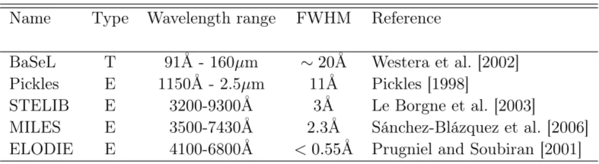
2.2 Examples of theoretical and empirical stellar libraries. We report name, type, wavelength range, FWHM around 5500 Å and reference. 30 2.3 Average temperatures and densities of the gas in the interstellar

medium in diﬀerent phases. . . 33 3.1 Prior distributions of the current (i.e. averaged over the last 10 Myr)

physical properties of star-forming galaxies in the library of star for-mation and chemical enrichment histories assembled in Sections 3.2.1 and 3.2.2. . . 64 3.2 Summary of the constraints on galaxy physical parameters retrieved

from different types of optical observations using the method devel-oped in Section 3.2. For each parameter and each type of observation, the quoted uncertainty (defined as half the 16th–84th percentile range of the retrieved likelihood distribution) and accuracy (defined as the absolute difference between the retrieved best estimate and true pa-rameter value) are median quantities determined from the analysis of 10,000 pseudo-observations in Section 3.3. . . 99 4.1 ID and spectroscopic redshifts of the galaxies in the sample described

in Section 4.2. . . 105 4.2 Scaling factors of the galaxies in the sample deﬁned as the ratio

be-tween the median flux in a square band of 0.1µm width, centered on the J-band effective wavelength, and the FIREWORKS mean flux in the J-band. . . 106 4.3 Differences in the prescriptions adopted in MAGPHYS and in the

(31)

(32)

Chapter 1

Introduction

"A Nebula is a celestial object, often of irregular form and brightness, appearing like a mass of luminous fog. ... Among elliptic nebulae, the signal object is the great nebula in Andromedae.", New Astronomy, Todd [1906].

1.1 The Universe

At the beginning of the 20th century, the measured distances towards objects in the sky were quite uncertain and the Milky Way was believed to be the only system in the Universe. In 1925, Edwin Hubble discovered that certain objects, called nebulae, were too far away to be part of the Milky Way. He suggested that the Universe extended much beyond our Galaxy and that those nebulae had intrinsic sizes similar to the Milky Way. The evidence that changed the vision of the Universe was that the light reaching us from distant galaxies is shifted to the red compared to what is seen in laboratories. This redshift is deﬁned as

z = λobs− λem λem

, (1.1.1)

where λem is the wavelength at which light is emitted by a distant galaxy and λobs

is the wavelength at which this light is detected by the observer. Hubble observed a correlation between the redshift and the distance of these galaxies, known as the Hubble law

cz = H0d , (1.1.2)

where cz is the recession velocity1

of the galaxy, d is the distance to the galaxy and H0 is the Hubble constant. Redshift can therefore be used as a measure of distance

to a galaxy. Hubble concluded also that extragalactic objects are moving away from the Milky Way [Hubble, 1929] and that the Universe is expanding.

The expansion of the Universe can be understood in the framework of Fried-mann’s solution to Einstein ﬁeld equations of general relativity2_{. In the standard}

model of Big Bang cosmology, the Universe expanded and cooled from a hot and dense initial state about 13.7 Gyr ago. It cooled suﬃciently to allow energy to be converted into various subatomic particles which then combined to form atoms.

1

This is based on the Doppler effect, ∆λ/λ = v/c and is valid for non-relativistic objects (z ≪ 1). This relation can be extended in special and general relativity, and be applied to objects with z > 1.

2

Einstein field equations describe gravitational interactions as a result of spacetime being curved by matter and energy.

(33)

Recent observations of the cosmic microwave background radiation and of distant supernovae suggest that this expansion is accelerating (see for example, Spergel et al. 2003, Lamarre et al. 2003, Riess et al. 1998) under the inﬂuence of a mysteri-ous dark energy. This component can be formalized with the cosmological constant Λ in Einstein equations3_.

The other main component that appears to be driving the evolution of the Universe is dark matter. Dark matter neither emits nor scatter light. It interacts only gravitationally and thus cannot be observed directly. The dark mass component revealed by the rotational curve of galaxies and by gravitational lensing looking through galaxy clusters are evidences of the presence of this dark matter.

In the standard model, cold (i.e. non-relativistic) dark matter accounts for ∼ 23 percent, while dark energy constitutes ∼ 72 percent of the mass-energy density of the Universe. Only the remaining 5 percent is in the form of visible baryonic matter (stars, gas and dust). The general idea is that dark matter structures grow from weak density fluctuations present in the homogeneous and rapidly expanding early universe. These fluctuations are amplified by gravity, turning into the structures that we observe today.

Although many cosmological simulations have been developed to describe the evolution of the baryons in these dark-matter structures, the complexity of the physical processes involved (gas cooling mechanisms, feedback, the process of star formation) has prevented the full understanding of the formation and evolution of the galaxies we see today.

Progress in this area has come mainly from the advent of deep sky observations at the end of the 20th century. In fact, because of the ﬁnite speed of light, the light reaching us from distant galaxies provides images from the past. Therefore, observations of large samples of galaxies at various redshifts should help us better understand the formation and evolution of galaxies in a hierarchical Universe.

1.2 Galaxies

Over the past two decades, the advent of large ground-based and space-based ob-servatories has largely improved our knowledge of galaxies. These obob-servatories have allowed us to probe the light emitted by galaxies at diﬀerent energies or wave-lengths, from γ-rays to radio. Figure 1.1 provides an overview of the current and future instruments enabling the collection of galaxy lights across the electromag-netic spectrum. In this thesis we focus on the observation of galaxies at ultraviolet, optical and near-infrared wavelengths. We now recall a few basic concepts about the interpretation of galaxy observations.

3

The cosmological constant was first proposed by Albert Einstein as a modification of his original theory of general relativity to achieve a stationary universe. Einstein abandoned the concept after Hubble discovered the expansion of the Universe. The discovery of a cosmic acceleration has recently renewed interest in Λ.

(34)

1.2. Galaxies 3

Figure 1.1: A broad view of the most important telescopes and the wavelength ranges they cover. The atmospheric absorption coeﬃcient is also shown.

1.2.1 Galaxy morphologies

A wide variety of galaxy shapes and colors can be observed in the Universe. Hubble compiled a classiﬁcation of galaxies based on morphology [Hubble, 1926]. In this scheme, galaxies are divided into ellipticals (E), lenticulars (S0), spirals (Sa, Sb, Sc, . . . ), barred spirals (SBa, SBb, SBc, . . . ) and irregulars (Irr). Ellipticals and lenticulars are also referred to as early-type galaxies, while spirals can be of either early type (Sa) or late type (Sc, . . . ). The morphology of galaxies tends to correlate with the color4

. Early-type galaxies generally look red, contain little gas and host negligible star-formation. Late-type galaxies contain more gas and dust and host a larger amount of young blue stars. Strateva et al. [2001] noted that local galaxies exhibit a bimodal distribution in color space: a red peak is populated mainly by non-star-forming galaxies of morphological type earlier than Sa; a blue peak is pop-ulated primarly by star-forming galaxies of morphological type later than Sb. At high redshift, morphological studies are more diﬃcult because galaxies have smaller apparent sizes.

1.2.2 Galaxy spectral energy distributions

Stars and the interstellar medium in galaxies emit radiation across the full electro-magnetic spectrum. As an example, Figure 1.2 shows images of the galaxy NGC1512 observed in diﬀerent bands from the ultraviolet to the infrared. The ultraviolet light reﬂects the emission from the youngest stars and is preferentially absorbed by

in-4

The color of a galaxy is defined as the ratio of the flux observed in a long-wavelength band and the flux observed in a short-wavelength band.

(35)

Figure 1.2: Photometric images of the galaxy NGC1512 in diﬀerent bands. Clock-wise from left to right: far ultraviolet (∼ 2000Å), near ultraviolet (∼ 3000Å), optical (∼ 5000Å), Hα emission (6563Å), near infrared (∼ 1µm), mid infrared (∼ 10µm) and far infrared (∼ 100µm). Credit: NASA.

(36)

1.2. Galaxies 5 terstellar dust. Older stars radiate mainly at longer wavelengths (near-infrared). The emission by gas is characterized by narrow emission lines (such as, Hα line at 6563Å). Dust absorbs and scatters the ultraviolet and optical light emitted by stars and gas, and reradiates this at mid- an far-infrared wavelengths (note that in Fig. 1.2 optical and infrared images are almost complementary).

The light emitted by galaxies at different wavelengths therefore contains valuable information about the properties of the stars, gas and dust within them. This light can be probed by means of different types of observations: integrating the flux through broad- and narrow-band filters (photometry), or dispersing the light in wavelength at different spectral resolutions (spectroscopy).

Figure 1.3a shows an example of spectral energy distribution of a galaxy at optical wavelengths. Overlaid are the five filter response functions, u g r i z, of the Sloan Digital Sky Survey (SDSS, York et al. 2000). The flux gathered through filters of this type is generally expressed in magnitudes. In this thesis, we always compute magnitudes in the AB system:

mag = −2.5 log₁₀fν− 48.6 , (1.2.3) where fν = Z dν hν SνFν Z dν hν Sν (1.2.4) is the mean photon weighted flux through the filter, expressed in erg per second per square centimeter per hertz, and Sν is the filter response function. Broad-band

photometric observations are usually characterized by good signal-to-noise ratio. They can trace the main features of galaxy spectral energy distributions.

More reﬁned information about galaxy spectral energy distributions, such as strong emission- and absorption-line features, can be obtained using narrow-band photometry (∼ 100Å band-width). For example, the equivalent widths of strong emission lines can be estimated by combining narrow-band and broad-band obser-vations. The equivalent width of a line is deﬁned as5

EW = Z λ2 λ1 dλFλ− Cλ Fλ , (1.2.5)

where λ1and λ2 deﬁne the wavelength range sampled by the line, Fλ is the observed

ﬂux per unit wavelength (that can be probed by narrow-band imaging) and Cλ is

the flux per unit wavelength of the continuum under the line (whose mean value can be estimated from broad-band imaging). An accurate flux calibration is not crucial when measuring equivalent widths, since they involve only flux ratios.

More detailed information about the emission and absorption features in galaxy spectral energy distributions can be gathered by appealing to spectroscopy (Fig. 1.3b). A disadvantage is that spectroscopy requires far more telescope time

5

(37)

Figure 1.3: Panel (a): spectral energy distribution of a galaxy at optical wavelengths (black line) overlaid are the ﬁve ﬁlter response functions of the SDSS. Panel (b): same spectral energy distribution as in panel (a) (black line), with the strongest emission lines labeled; the red line shows the stellar continuum underneath the lines. Panel (c): the same spectral energy distribution as in panel (a), computed at a 10-times lower resolution; red points mark the binning. Note that the ordinate scale in panel (c) is enlarged.

(38)

1.3. Outline 7 than photometry to reach similar signal-to-noise ratio. In this contest, low-resolution spectroscopy represents an interesting trade-oﬀ between broad-band photometry and high-resolution spectroscopy. As shown in Figure 1.3c, emission and absorption fea-tures in this case are still detectable, although disentangling these feafea-tures from the stellar continuum becomes problematic. A major contribution of this thesis is to develop a new approach to extract valuable information from low-resolution spectroscopic observations of galaxies.

1.3 Outline

In this thesis we investigate the relative merits of diﬀerent types of observations to constrain the stars, gas and dust content of galaxies. Our main motivation is to extract the best constraints from the large amount of high-quality data that are being gathered on galaxies at various redshifts using modern telescopes, as well as to help plan for future galaxy surveys. To this aim, we develop an original approach to characterize physical properties of galaxies, e.g. stellar mass, star formation history, gas-phase metallicity, based on the combined interpretation of the stellar and nebular emission. A main feature of our approach is the high level of sophistication of the prescriptions used to build a comprehensive library of galaxy spectral energy distributions.

In Chapter 2, we introduce the diﬀerent tools involved in the modeling of spec-tral energy distributions of galaxies. We show how physically motivated star for-mation and chemical enrichment histories can be derived from the semi-analytic post-treatment of a large-scale cosmological simulation. Also, we show how state-of-the-art models of stellar spectral synthesis, nebular emission and attenuation by dust can be used to describe the emission from stars and the interstellar medium in galaxies.

In Chapter 3, we present a new approach to constrain galaxy physical parame-ters from the combined interpretation of the stellar and nebular emission, using a comprehensive library of model spectral energy distributions. We appeal to pseudo-observations to assess the relative merits of photometric and spectroscopic observa-tions, to constrain galaxy physical parameters. Then, we apply our approach to the interpretation of a sample of ∼13,000 high quality SDSS galaxies.

In Chapter 4, we further apply our approach to the analysis of a sample of 12 spectra extracted from an ongoing survey of high-redshift galaxies with the new wide ﬁeld camera on board the Hubble Space Telescope (3D-HST, PI Dr. Pieter van Dokkum). The sample consists of star-forming galaxies at z ∼ 2, observed in the optical rest-frame at low resolution and low signal-to-noise ratio. We compare our estimates of stellar mass and speciﬁc star formation rate with estimates derived using a photometric approach. This analysis is part of a project started in November 2011 with Dr. Elisabete da Cunha and Prof. Hans-Walter Rix, and it is to be concluded in summer 2012.

(39)

even higher redshifts selected among the deepest photometric observations in the Hubble Ultra Deep Field. The sample consists of 55 galaxies in the redshift range 2 < z < 8 observed at optical and near-infrared wavelengths. We focus in particular on the correlation between the shape of the rest-frame ultraviolet spectral energy distribution and the optical depth of the dust.

In Chapter 6, we summarize this work and present our conclusions.

More detail about some technical points can be found in Appendices A and B. The photometric data used in Chapter 5 are listed in Appendix C.

(40)

1.3.

Outline

9

PHYSICAL PARAMETERS

mass, star formation history, metal and

dust content... SED-interpretation techniques Bayesian Pseudo-observations instrument response function, signal-to-noise ratio... accuracy and uncertainty in estimates of physical parameters as a function of: prior, quality of data,

availability of data MODELS PRIOR PR IO R Plan galaxy observations DATA sets of observables (imaging, spectroscopy) Empirical relations Theory of galaxy formation and evolution

SFH, stellar emission, nebular emission, attenuation by dust

(41)

(42)

Chapter 2

Modeling galaxy spectral energy

distributions

The modeling of the light emitted by the different constituents of galaxies (stars, gas and dust) is required to interpret multi-wavelength observations in terms of constraints on physical parameters, such as star formation rate, metallicity and dust content. In this Chapter, we introduce the different types of techniques that have been developed to model the spectral energy distributions of galaxies, with the goal to constrain the histories of star formation and chemical enrichment. In Section 2.1, we introduce different approaches to study the star formation history of galaxies. In Section 2.2, we describe models of the emission from stellar populations, and in Section 2.3, models of the emission from the gas heated by young stars. The effects of dust on the light emitted by stars and gas are addressed in Section 2.4. At the end (Section 2.5), we also mention the necessity to account for absorption by the intergalactic medium when modeling the emission from distant galaxies.

2.1 The star formation history of galaxies

The star formation history is the evolution of the rate of star formation as a func-tion of galaxy age. The light arising from a galaxy should reflect the past episodes of star formation it underwent, through the spectral signatures of different stellar generations and the implied enrichment of the interstellar medium. Dissecting the integrated light of an individual galaxy into components of different ages is a com-plicated process. If one considers the galaxy population as a whole, a more direct way to gain at least some clues on the global star formation history of the Universe is to explore the star formation rate density at different cosmic epochs. This can be achieved because measurements of the current rate of star formation at any cosmic epoch through the emission from bright young stars is less challenging than inter-preting the spectral signatures of old stars in the spectra of today’s galaxies. To interpret, instead, the evolution of individual galaxies, requires more complicated models of the history of star formation. In this Section, we first briefly recall the con-clusions that can be drawn from analyses of the global star formation rate density of the Universe at various cosmic epochs and the different sources of uncertainty affecting these analyses. Then, we describe in more detail the models that have been developed to follow the star formation and chemical enrichment histories of individual galaxies, in the framework of a hierarchical universe, and the successes and limitations of such models.

(43)

2.1.1 The star formation history of the Universe

The study of the star formation history of galaxies through the assessment of the star formation rate density at diﬀerent epochs has been pioneered by Lilly et al. [1996] and Madau et al. [1996], combining observations from the local Universe to z ∼ 3−4. Hopkins [2004] and Hopkins and Beacom [2006] have improved the statistics out to z ∼ 6 and have analyzed the various sources of uncertainties that can contribute to the normalization of the star formation rate density. More recently, Cucciati et al. [2011] have investigated the star formation rate density from z ∼ 0.05 to z ∼ 4.5 using data from a single galaxy redshift survey (VIMOS-VLT Deep Survey, VVDS, Garilli et al. 2008, Le Fèvre et al. 2004, Le Fèvre et al. 2005), to avoid merging diﬀerent datasets. In their work, they assess also the various sources of uncertainties, and in particular, the treatment of dust attenuation.

In Figures 2.1 and 2.2, respectively, we present the original and the most recent determinations of the evolution of the star formation rate density of the Universe as a function of redshift. Despite the inhomogeneity of the galaxy samples used in these studies and the diﬀerences in the adopted star-formation-rate indicators (far ultraviolet, far infrared, Hα emission line luminosity, radio observations), the Universe appears to have undergone a phase of most active star formation around z ∼ 1 − 2. Other uncertainties aﬀect this measurement, leading to large error bars. For example, the correction for attenuation by dust at ultraviolet and optical wavelengths and the interpretation of dust emission at infrared wavelengths can alter estimates of the star formation rate. Moreover, the lack of statistics beyond redshift of 2–3 precludes the interpretation of the decline of star-formation at cosmic epochs earlier than z ∼ 1.

Although the evolution of the star formation rate density gives us important clues about the global history of star formation of the Universe, the interpretation of the results of Figures 2.1 and 2.2 is very limited. To gain more insight into the evolution of diﬀerent types of galaxies, we thus need to investigate in more detail the star formation history of individual galaxies.

2.1.2 The star formation history of individual galaxies

Constraining the star formation history of individual galaxies requires models that can describe the spectral evolution implied by different scenarios of star formation and chemical enrichment. By comparing such models with observations, one can infer the most likely scenario for the evolution of individual galaxies. In practice, even idealized representations of the star formation history can reproduce reasonably well the colors of nearby galaxies. Here, we first briefly describe different idealized representations of the star formation history of individual galaxies. We then describe more sophisticated approaches based on detailed cosmological simulations.

(44)

2.1. The star formation history of galaxies 13

Figure 2.1: Fig. 9 from Madau et al. [1996], showing on the left the Universal metal ejection density, ˙ρZ, and on the right the total star formation rate density, ˙ρ∗, as a

function of redshift. Triangle: Gallego et al. [1995]. Filled dots: Lilly et al. [1996]. Filled squares: lower limits from Hubble Deep Field images.

Figure 2.2: Fig. 5 from Cucciati et al. [2011], showing the total dust-corrected UV-derived star formation rate density as a function of redshift from the VVDS sample (red ﬁlled circles). The black dashed line is the star formation rate density as a function of z implied from the stellar mass density in Ilbert et al. [2010]. Other data sets are overplotted and labeled on the ﬁgure. All data have been converted into a star formation rate density with the scaling relation from Madau et al. [1998].

(45)

2.1.2.1 Simple idealized models of star formation history

Galaxy star formation histories have been traditionally approximated by simple analytic functions: single bursts of star formation, constant star formation rate, ex-ponentially declining star formation rate or a combination of these three. Figure 2.3 shows 3 templates of star formation histories and the corresponding spectral en-ergy distributions, computed using the latest version of Bruzual and Charlot [2003] for ﬁxed solar metallicity, with a Chabrier initial mass function [Chabrier, 2003]. Emission lines are computed consistently following the prescription by Charlot and Longhetti [2001]. Attenuation by dust is neglected in this example. A constant star formation history (panel a) gives a relatively blue spectral energy distribution (panel e). A single burst of star formation at early times (panel b) does not include the emission from any young stars, resulting in a fairly red spectral energy distribution (panel e). In panel (c), we show an exponentially declining star formation history, with e-folding time 2.5 Gyr, and the corresponding spectral energy distribution is shown in panel (f).

Previous studies (e.g. Kauffmann et al. 2003a, Brinchmann et al. 2004, da Cunha et al. 2008) have shown that these simplistic formulations of star formation histories are able to reproduce the colors of low-redshift galaxies. For example, Kauffmann et al. [2003a] show that exponentially declining star formation histories, with random superimposed bursts of star formation, reproduce reasonably well the colors of a representative sample of galaxies from the SDSS at redshift 0.03 and 0.11, once corrected for dust attenuation (see Figure 2.4). We note that these authors also correct the SDSS colors for the contamination by emission lines. We will return in Chapter 3 (Figure 3.7) on the non-negligible influence of nebular emission lines when interpreting the observed colors of star-forming galaxies.

Wuyts et al. [2009] speciﬁcally investigate the limitations arising from the in-terpretation of complex star formation histories of galaxies using idealized repre-sentations of the type shown in Figure 2.3. Their approach consists of 2 steps: 1 – building ‘realistic’ galaxy spectral energy distributions based on star formation histories derived from a sophisticated simulation of galaxy formation (they adopt a simulation based on a smoothed-particle-hydrodynamic code, see Section 2.1.2.2); 2 – comparing the colors of these galaxies with colors of model galaxies computed using simplistic star formation histories. They consider the spectral evolution over a period of only 2 Gyr, as they focus on studies of high-redshift galaxies. Wuyts et al. [2009] show that the spectral energy distributions of galaxies derived from a cosmological simulation are better represented by exponentially declining star for-mation histories with e-folding time of 300 Myr than by single-burst and constant star formation histories. They also ﬁnd that, in the case of starburst galaxies, age and mass are systematically underestimated when adopting simple exponentially declining star formation histories. They show that models allowing for secondary bursts of star formation on top of an exponentially declining star formation history allow for larger total stellar masses, providing a better match for blue objects than without secondary bursts (see also Papovich et al. 2006, Erb et al. 2006, Wuyts