Auction algorithms for network flow problems : a tutorial introduction

May 1992 LIDS - P - 2108

Auction Algorithms for Network Flow Problems:

A Tutorial Introduction 1

by

Dimitri P. Bertsekas2

Abstract

This paper surveys a new and comprehensive class of algorithms for solving the classical linear network flow problem and its various special cases such as shortest path, max-flow, assignment, transportation, and transhipment problems. The prototype method, from which the other algorithms can be derived, is the auction algorithm for the assignment problem. This is an intuitive method that operates like a real auction where persons compete for objects by raising their prices through competitive bidding; the prices can be viewed as dual variables. Conceptually, auction algorithms represent a significant departure from the cost improvement idea that underlies primal simplex and dual ascent methods; at any one iteration, they may deteriorate both the primal and the dual cost. Auction algorithms perform very well for several important types of problems, both in theory and in practice, and they are also well suited for parallel computation.

1 Research supported by NSF under Grant No. DDM-8903385 and Grant CCR-9103804, and by the ARO under Grant DAAL03-86-K-0171.

Contents

1. Introduction ... p... p. 4

2. Assignment by Naive Auction ... p...p. 5

The Naive Auction Algorithm . ... 6

3. e-Complementary Slackness and the Auction Algorithm . ... p. 7

The Auction Algorithm ... ... 8

c-Scaling. ... . . . ... . .. ... p.. p10

Dealing with Infeasibility .. . ... p. 12

Profits and Reverse Auction .. ... p. 14

Combined Forward and Reverse Auction ... p. 15

4. Auction Algorithms for Shortest Path Problems . ... p. 17

The Auction/Shortest Path Algorithm ... ... p. 19

The Reverse Algorithm . . .... ... . ... p.21

The Auction Algorithm with Graph Reduction .... . .... . p.23

k Shortest Path Problems ... p. 24

k Node-Disjoint Shortest Path Problems ... . ... ... p.24

5. Extension to Transportation Problems ... p. 25

The Auction Algorithm with Similar Objects ... . .. p... p. 27

The Auction Algorithm with Similar Persons . .. . . p... p. 28

6. A Generic Auction Algorithm for Minimum Cost Flow Problems ... p. 30

The Generic Algorithm ... ... p. 34

7. The e-Relaxation Method ... p. 34

8. Application of the e-Relaxation Method to Max-Flow Problems . . . . . ... p. 35 9. Extension to Asymmetric Assignment Problems . ... p. 36 Reverse Auction for Asymmetric Assignment Problems. ... p. 37 Forward/Reverse Auction for Other Types of Inequality Constrained Problems. . . p. 39 10. Practical Computational Aspects of Auction Algorithms . . . . . . . . ... p. 39

10.1. Assignment Problems .. . . . p. 39

Adaptive e-Scaling . ... p. 39

The Problem of Integer Overflow ... .. ... . . . p. 40..

The "Third Best" Implementation. ... p. 40

Parallel and Asynchronous Implementation ... . . .. . p. 41

10.2. Shortest Path Problems ... ... p. 43

Parallel Implementation ... . . . p. 44

10.3. Transportation Problems. ... p. 45

10.4. Minimum Cost Flow Problems ... p. 45

10.5. Max-Flow Problems ... .. ... p. 46

11. Conclusions ... p. 46

Appendix 1: c-CS, Primal Optimality, and Dual Optimality ... p. 50

Assignment Problems . . . . ... ... p. 50

Minimum Cost Flow Problems ... p. 51

1. Introduction 1. INTRODUCTION

The classical algorithms for solving linear network flow problems are primal cost improvement methods, including simplex methods, which iteratively improve the primal cost by moving flow around simple cycles, and dual ascent methods, which iteratively improve the dual cost by changing the prices of a subset of nodes by equal amounts.

Auction algorithms, the subject of this tutorial paper, are fundamentally different; they depart from the cost improvement idea and at any one iteration, they may deteriorate both the primal and the dual cost, although in the end they find an optimal primal solution. Their origin lies in nondifferentiable optimization (where nonmonotonic subgradient-based algorithms are common), and in the e-subgradient method of Bert-sekas and Mitter [BeM73] in particular (where the progress of the method depends on gradually reducing an e parameter to an acceptable tolerance level). Auction algorithms are also highly intuitive and easy to understand; they can be explained in terms of economic competition concepts, which are couched on everyday experience.

Auction algorithms originated in 1979 with an algorithm proposed by the author for the classical as-signment problem [Ber79]. This algorithm was further developed in [Ber85], [Ber88], and [BeE88]. The motivation was to solve the problem by using parallelism in a natural way. It turned out, however, that the resulting method was very fast in a serial environment as well. Subsequent work extended the auction algorithm to other linear network flow problems. In particular, an extension to the minimum cost problem, the e-relaxation method, was given by the author in [Ber86a] and [Ber86b]. An auction algorithm for trans-portation problems was given by the author in collaboration with D. Castaiion in [BeC89a]. An auction algorithm for shortest paths was given by the author in [Ber91lb]. Finally, a max-flow algorithm, developed by Goldberg [Gol85] from an entirely different point of view, fundamentally involves auction ideas and can be viewed as the natural extension of the auction algorithm to the max-flow problem.

All of the algorithms just mentioned can be derived from the original 1979 auction algorithm for the assignment problem. The derivation is based on well-known transformations of the general linear minimum cost flow problem and its various special cases (e.g., shortest path, max-flow, etc.) to equivalent assignment problems. Once the auction algorithm is applied to the corresponding equivalent assignment problem and the computations are streamlined, one obtains an auction algorithm for the original problem.

The purpose of this paper is to provide a tutorial introduction to auction algorithms. For textbook presentations, we refer the reader to [BeT89] and [Ber91a]. We will initially focus on the basic algorithm for the assignment problem, and then discuss various extensions to other problems. In Sections 2 and 3, we develop the auction algorithm for the symmetric assignment problem. In particular, we discuss a number of issues that are common to all types of auction algorithms, including e-scaling, and dealing with infeasibility. We also discuss an alternative form of the auction algorithm, called reverse auction; while in regular auction persons bid for objects by raising their prices, in reverse auction objects compete for persons by essentially offering discounts. In Section 4 we develop auction algorithms for shortest path problems. In Section 5, we discuss the extension of the auction algorithm to transportation problems, and in Section 6 we give a generic auction algorithm for the minimum cost network flow problem. In Section 7, we develop the

2. Assignment by Naive Auction relaxation method for the minimum cost flow problem as a special case of the generic algorithm. The e-relaxation method is specialized to the max-flow problem in Section 8, yielding algorithms similar to those of Goldberg and Tarjan [Gol85], [GoT86]. In Section 9 we discuss specialized auction algorithms for inequality constrained problems such as the asymmetric assignment problem. Finally, in Section 10 we discuss the computational aspects of auction algorithms, including issues of parallel and asynchronous implementation.

2. ASSIGNMENT BY NAIVE AUCTION

In the classical symmetric assignment problem there are n persons and n objects that we have to match on a one-to-one basis. There is a benefit ad for matching person i with object j and we want to assign persons to objects so as to maximize the total benefit. We are given a set A of pairs (i,j) that can be matched. For each person i, we denote by A(i) the set of objects that can be matched with i

A(i) = {j

I

and for each object j, we denote by B(j) the set of persons that can be matched with j

B(j) = {i

I

By an assignment we mean a set S of person-object pairs (i, j) such that each person i and each object j is involved in at most one pair from S. If the number of pairs in S is n, so that every person is assigned to a distinct object, we say that S is feasible; otherwise S is said to be infeasible. If a feasible assignment exists the problem is said to be feasible, and otherwise it is said to be infeasible. We seek a feasible assignment [a set of person-object pairs (1, j),.. ., (n,jn) from A, such that the objects il, ... , jn are all distinct], which is optimal in the sense that it maximizes the total benefit n=l aij,.

The symmetric assignment problem should be distinguished from its asymmetric version where the number of objects is larger than the number of persons, and while there is a requirement to assign every person, there is no such requirement for the objects. Auction algorithms for asymmetric and other related assignmment problems will be discussed in Section 9.

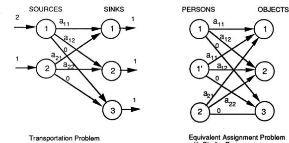
The assignment problem is important in many practical contexts, but it is also of great theoretical importance. Despite its simplicity, it embodies a fundamental linear programming structure. One of the most important type of linear programming problem, the minimum cost network flow problem, can be reduced to the assignment problem by means of a simple reformulation (see e.g. [BeT89], p. 335, [Ber91la], p. 17, [PaS82], p. 149, and Section 6). Thus, any method for solving the assignment problem can be generalized to solve the minimum cost flow problem. For this reason, the assignment problem has served as a convenient starting point for important algorithmic ideas in linear programming. For example, the primal-dual method ([FoF62], [Min60]), was motivated and developed through Kuhn's Hungarian method [Kuh55], the first specialized method for the assignment problem.

To develop an intuitive understanding of the auction algorithm, it is helpful to introduce an economic equilibrium problem that turns out to be equivalent to the assignment problem.

2. Assignment by Naive Auction

Consider the possibility of matching the n objects with the n persons through a market mechanism, viewing each person as an economic agent acting in his/her own best interest. Suppose that object j has a price pj and that the person who receives the object must pay the price pi. Then, the (net) value of object

j for person i is aij - pj and each person i would logically want to be assigned to an object ji with maximal

value, that is, with

aj, - Pi = max (aii -pj}. (1)

jEA(i)

The economic system would then be at equilibrium, in the sense that no person would have an incentive to act unilaterally, seeking another object.

Equilibrium assignments and prices are naturally of great interest to economists, but there is also a fun-damental relation with the assignment problem; it turns out that an equilibrium assignment offers maximum

total benefit (and thus solves the assignment problem), while the corresponding set of prices solves an asso-ciated dual problem. This is a consequence of the duality theorem of linear programming (see e.g. [Dan63],

[PaS82], [Lue84]). In the terminology of linear programming, relation (1) is known as complementary

slack-ness (CS for short). A simple, first principles proof of the relation of equilibria to optimal assignments and

dual optimization is also developed in Appendix 1.

The Naive Auction Algorithm

Let us consider a natural process for finding an equilibrium assignment and price vector. We will call this process the naive auction algorithm, because it has a serious flaw, as will be seen shortly. Nonetheless, this flaw will help motivate a more sophisticated and correct algorithm.

The naive auction algorithm proceeds in iterations and generates a sequence of price vectors and assign-ments. At the beginning of each iteration, the CS condition

aij, - Pi, = max {aij - pj} (2)

jEA(i)

is satisfied for all pairs (i, j,) of the assignment. If all persons are assigned, the algorithm terminates. Otherwise a nonempty subset I of persons i that are unassigned is selected and the following computations are performed.

Typical Iteration of Naive Auction Algorithm

Let I be a nonempty subset of persons that are unassigned.

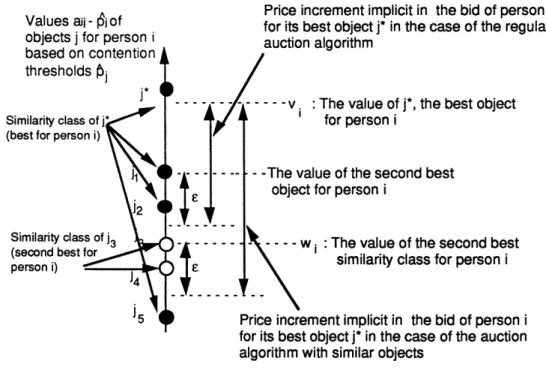
Bidding Phase: Each person i E I finds an object ji which offers maximal value, that is,

3i E arg max({aij-pj}, (3)

jEA(i)

and computes a bidding increment

Yi = v, - wi, (4)

where vi is the best object value,

vi = max ai' -pj}, (5)

3. e-Complementary Slackness and the Auction Algorithm and w, is the second best object value

w, = max {aij - pj). (6)

[If j; is the only object in A(i), we define wi to be -oo or, for computational purposes, a number that is much smaller than v,.]

Assignment Phase: Each object j that is selected as best object by a nonempty subset P(j) of persons in I, determines the highest bidder

ij = arg max yi, (7)

iEP(j)

raises its prices by the highest bidding increment maxiEp() -i, and gets assigned to the highest bidder ij; the person that was assigned to j at the beginning of the iteration (if any) becomes unassigned.

The algorithm continues with a sequence of iterations until all persons have an assigned object.

Note that 7, cannot be negative since v, > wi [compare Eqs. (5) and (6)], so the object prices tend to increase. In fact, when i is the only bidder, yi is the largest bidding increment for which CS is maintained following the assignment of i to his/her preferred object. Just as in a real auction, bidding increments and price increases spur competition by making the bidder's own preferred object less attractive to other potential bidders.

Note also that there is some freedom in choosing the subset of persons I that bid during an iteration. One possibility is to let I consist of a single unassigned person. This version, known as the Gauss-Seidel version because of its similarity with Gauss-Seidel methods for solving systems of nonlinear equations, usually works best in a serial computing environment. The version where I consists of all unassigned persons, is the one best suited for parallel computation; it is known as the Jacobi version because of its similarity with Jacobi methods for solving systems of nonlinear equations.

3. e-COMPLEMENTARY SLACKNESS AND THE AUCTION ALGORITHM

Unfortunately, the naive auction algorithm does not always work (although it is an excellent initialization procedure for other methods that are based on price adjustment, e.g. primal-dual or relaxation). The difficulty is that the bidding increment yi is zero when more than one object offers maximum value for the bidder i. As a result, a situation may be created where several persons contest a smaller number of equally desirable objects without raising their prices, thereby creating a never ending cycle; see Fig. 1.

To break such cycles, we introduce a perturbation mechanism, motivated by real auctions where each bid for an object must raise the object's price by a minimum positive increment, and bidders must on occasion take risks to win their preferred objects. In particular, let us fix a positive scalar c and say that an assignment and a price vector p satisfy e-complementary slackness (or c-CS for short) if

aq, - Pji > max Iaij - pj} - e, (8)

jEA(i)

for all assigned pairs (i, j,). In words, to satisfy e-CS, all assigned persons must be assigned to objects that are within e of being best.

3. c-Complementary Slackness and the Auction Algorithm

PERSONS OBJECTS

Initially assigned Initial price = 0

to object 1

Initially assigned Initial prce

to object 2

Here a = C > O for all (i,j) with i = 1,2,3 and j = 1,2 and aij J 0 for all (i,j) with I = 1,2,3 and j = 3 Initially

unassigned Initial price =

At Start of Object Assigned Bidder Preferred Bidding

Iteration # Prices Pairs Object Increment

1 0,0,0 (1,1), (2,2) 3 2 0

2 0,0,0 (1,1), (3,2) 2 2 0

3 0,0,0 (1,1), (2,2) 3 2 0

Figure 1: Illustration of how the naive auction algorithm may never terminate for a three person and three object problem. Here objects 1 and 2 offer benefit C > 0 to all persons, and object 3 offers benefit 0 to all persons. The algorithm cycles as persons 2 and 3 alternately bid for object 2 without changing its price because they prefer equally object 1 and object 2 (y, = 0).

The Auction Algorithm

We now reformulate the previous auction process so that the bidding increment is always at least equal to e. The resulting method, the auction algorithm, is the same as the naive auction algorithm, except that the bidding increment 7, is

7i = vi - wi + e, (9)

[rather than -y = v, - w, as in Eq. (4)]. With this choice, the e-CS condition is satisfied. The particular increment 7i = vi - wi + E used in the auction algorithm is the maximum amount with this property. Smaller increments yi would also work as long as yi > c, but using the largest possible increment accelerates the algorithm. This is consistent with experience from real auctions, which tend to terminate faster when the bidding is aggressive.

It can be shown that this reformulated auction process terminates in a finite number of iterations, nec-essarily with a feasible assignment and a set of prices that satisfy e-CS. To see this for the case of a fully dense problem (A consists of all person-object pairs), note that if an object receives a bid in k iterations, its price must exceed its initial price by at least ke. Thus, for sufficiently large k, the object will become "expensive" enough to be judged "inferior" to some object that has not received a bid so far. It follows an object can receive a bid in a limited number of iterations while some other object still has not yet received any bid. On the other hand, once all objects receive at least one bid, the auction terminates. Thus, the

3. e-Complementary Slackness and the Auction Algorithm auction algorithm must terminate, and in fact the preceding argument shows that, for the case of zero initial prices, the total number of iterations in which an object receives a bid is no more than

max(ij) laij I

If each iteration involves a bid by a single person, the total number of iterations is no more than n times the preceding quantity, and since each bid requires O(n) operations, the running time of the algorithm is

O(n2 max(ij) laijl/e).

This proof can be generalized for the case of a sparse problem (one where the set of person-object pairs that can be assigned is limited), as long as the problem is feasible; see Appendix 2. Figure 2 shows how the auction algorithm, based on the bidding increment y, = vi - wu + e [cf. Eq. (9)], overcomes the cycling problem of the example of Fig. 1.

PERSONS OBJECTS

Initially assigned( Initial price = 0

to object 1

Initially assigned Inital price =

to object 2

Here al = C > 0 for all (i,j) with i = 1,2,3 and j = 1,2

and aj = O for all (i.j) with i = 1,2,3 and j = 3

Initially Iniial price = 0

At Start of Object Assigned Bidder Preferred Bidding

Iteration

#

1 0,0,0 (1,1), (2,2) 3 2 e

2 0,e,0 (1,1), (3,2) 2 1 2e

3 2e,e,0 (2,3), (3,1) 1 2 2e

4 2c,3c,0 (1,2), (2,1) 3 1 2e

5 4e,3e,0 (1,3), (3,2) 2 2 2e

Figure 2: Illustration of how the auction algorithm overcomes the cycling problem for the example of Fig. 1, by making the bidding increment at least equal to c. The table shows one possible sequence of bids and assignments generated by the auction algorithm, starting with all prices equal to 0. At each iteration except the last, the person assigned to object 3 bids for either object 1 or 2, increasing its price by e in the first iteration and by 2e in each subsequent iteration. In the last iteration, after the prices of 1 and 2 rise at or above C, object 3 receives a bid and the auction terminates.

When the auction algorithm terminates, we have an assignment satisfying e-CS, but is this assignment optimal? The answer here depends strongly on the size of c. In a real auction, a prudent bidder would

3. e-Complementary Slackness and the Auction Algorithm not place an excessively high bid for fear that he/she might win the object at an unnecessarily high price. Consistent with this intuition, we can show that if e is small, then the final assignment will be "almost optimal." In particular, the following proposition (proved in Appendix 1) shows that the total cost of the

final assignment is within ne of being optimal. The idea is that when a feasible assignment and a set of prices

satisfy e-CS, they also satisfy CS (and are therefore primal and dual optimal, respectively) for a slightly

perturbed problem where all costs a,j are the same as before, except for the costs of the n assigned pairs,

which are modified by an amount no more than e.

Proposition 1: A feasible assignment satisfying c-complementary slackness together with some price vector is within nc of being optimal.

Suppose now that the costs a,, are all integer, which is the typical practical case (if aii are rational numbers, they can be scaled up to integer by multiplication with a suitable common number). Then, the total benefit of any assignment is integer, so if ne < 1, any complete assignment that is within ne of being optimal must be optimal. It follows, that if e < 1/n, and the benefits aij are all integer, then the assignment obtained upon termination of the auction algorithm is optimal. We state this result as a proposition; the proof is given in Appendix 2.

Proposition 2: Consider a feasible assignment problem with integer benefits aii. If

e <-,

n

the auction algorithm terminates in a finite number of iterations with an optimal assignment.

Figure 3 shows the sequence of generated object prices for the example of Figs. 1 and 2 in relation to the contours of the dual cost function of the assignment problem, which is given in Appendix 1. It can be seen from this figure that with each bid, the dual cost is approximately minimized (within e) with respect

to the price of the object receiving the bid. This observation can be established in generality; see [Ber88] or [Ber9 la]. Successive minimization of a cost function along single coordinates is a central feature of coordinate descent and relaxation methods, which are popular for unconstrained minimization of smooth functions and for solving systems of smooth equations. Thus, the auction algorithm can be interpreted as an approximate coordinate descent method.

e-Scaling

The amount of work needed for the auction algorithm to terminate can depend strongly on the value of e and on the maximum absolute object benefit C given by

C = max la;i1. (10)

(ij)E4

Basically, for many types of problems, the number of iterations up to termination tends to be proportional to C/e as argued earlier for fully dense problems. This can also be seen from the example of Fig. 3, where the number of iterations up to termination is roughly C/e, starting from zero initial prices. For small e,

3. e-Complementary Slackness and the Auction Algorithm

Contours of the dual function

i p.

Figure 3: A sequence of prices pl and P2 generated by the auction algorithm for the example of Figs. 1 and 2. The figure shows the equal dual cost surfaces in the space of pl and P2, with P3 fixed at 0.

the method is susceptible to "price wars", that is, protracted sequences of small price rises resulting from groups of persons competing for a smaller number of roughly equally desirable objects.

Note also that there is a dependence on the initial prices; if these prices are "near optimal," we expect that the number of iterations to solve the problem will be relatively small. This can be seen from the example of Fig. 3; if the initial prices satisfy P, - p3 + C and P2 ; p3 + C, the number of iterations up to

termination is quite small.

The preceding observations suggest the idea of e-scaling, which consists of applying the algorithm several times, starting with a large value of e and successively reducing e up to an ultimate value that is less than some critical value (for example, l/n, when the benefits aij are integer). Typical e-reduction factors after each scaling phase are of the order of 4 to 10. Each application of the algorithm provides good initial prices for the next application. e-scaling was suggested in the original proposal of the auction algorithm [Ber79], based on extensive experimentation, which established its effectiveness for many types of assignment problems. In particular, e-scaling is typically beneficial for sparse problems. The cost structure of the problem is also important in determining whether e-scaling is needed.

For integer data, it can be shown that the worst-case running time of the auction algorithm using scaling and appropriate data structures is O(nA log(nC)); see [BeE88], [BeT89]. Based on experiments, the running time of the algorithm for randomly generated problems seems to grow proportionally to something like

Alogn or A lognlog(nC). This is also supported by an approximate analysis in [Sch90O]. The practical

3. e-Complementary Slackness and the Auction Algorithm Dealing with Infeasibility

Since termination can only occur with a feasible assignment, when the problem is infeasible, the auction algorithm will keep on iterating, as the user is wondering whether the problem is infeasible or just hard to solve. Thus for problems where existence of a feasible assignment is not known a priori, one must supplement

the auction algorithm with a mechanism to detect infeasibility. There are several such mechanisms, which we will now discuss.

A basic result about (symmetric and asymmetric) assignment problems is that given an infeasible assign-ment S, there are two mutually exclusive possibilities:

(a) S has maximal cardinality, that is, there is no assignment having more assigned persons than S.

(b) There exists some unassigned person i and some unassigned object j and an augmenting path with respect to S that starts at i and ends at j, that is, a sequence of the form

(i, l il . .jra im,j)..

such that jl E A(i), j E A(im), and jk is assigned to ik under S for k = 1,..., m.

This result can be proved in a number of ways. For example, by introducing in the assignment problem graph a supersource node s connected to all the person nodes and a supersink node t connected to all the object nodes, we can view the problem of finding an assignment of maximal cardinality as the problem of finding a maximum flow from s to t. The result then follows by using the max-flow/min-cut theorem and the related analysis (eg., [Ber91la], Chapter 1, Props. 2.3 and 2.4).

A corollary of the preceding result is that given a feasible assignment problem and an infeasible assignment

S, for every person i that is unassigned under S, there exists an augmenting path with respect to S that

starts at i. (To prove this, modify S by assigning every person that is unassigned under S, except i, to a fictitious object, and then apply the preceding result.)

One criterion that can be used to detect infeasibility is based on the maximum values

i = max ai'--pj}

jEA(s)

It turns out that in the course of the auction algorithm, all of these values will be bounded from below by precomputable bound when the problem is feasible, but some of these values will be eventually reduced elow this bound if the problem is infeasible. In particular, suppose that the auction algorithm is applied with initial object prices {p0}. Then it can be shown that for any i, if person i is unassigned with respect to the current assignment S, and there is an augmenting path with respect to S that starts at i, we have

vi > -(2n- 1)C-(n- 1)e-max{p3}, (11)

where C = max(ij)EA la, l. The proof is obtained by adding the e-CS condition along the augmenting path. If the problem is feasible, then as discussed earlier, there exists an augmenting path starting at each unassigned person at all times, so the lower bound (11) on vi will hold for all unassigned persons i throughout

3. e-Complementary Slackness and the Auction Algorithm the auction algorithm. On the other hand, if the problem is infeasible, some persons i will be submitting bids infinitely often, and the corresponding values vi will be decreasing towards -oo. Thus, we can apply the auction algorithm and keep track of the values vi as they decrease. Once some vi gets below its lower bound, we know that the problem is infeasible.

Unfortunately, it may take many iterations for some vi to reach its lower bound. An alternative method to detect infeasibility is to convert the problem to a feasible problem by adding a set of artificial pairs `A to the original set A. The benefits of these pairs should be very small, so that none of them participates in an optimal assignment unless the problem is infeasible. In particular, it can be shown that if the original problem was feasible, no pair (i, j) E A will participate in the optimal assignment, provided that

a,j < -(2n - 1)C, V (i, j) E .A, (12)

where C = max(i;)EA la,jl. To prove this by contradiction, assume that by adding to the set A the set of artificial pairs .A we create an optimal assignment S* that contains a nonempty subset S of artificial pairs. Then, for every assignment S consisting exclusively of pairs from the original set A we must have

SE

(tj)ES (.ij)Es'- (ij)ES from which

5

E

This contradicts Eq. (12). Note that if aij > 0 for all (i,j) E A, the preceding argument can be modified to show that it is sufficient to have a,i < -(n - 1)C for all artificial pairs (i, j).

On the other hand, the addition of artificial pairs with benefit -(2n - 1)C as per Eq. (12) expands the cost range of the problem by a factor of (2n - 1). In the context of c-scaling, this necessitates a much larger starting value for e and correspondingly large number of e-scaling phases. If the problem is feasible these extra scaling phases are wasted. Thus for problems which are normally expected to be feasible, it may be better to introduce artificial pairs with benefits that are of the order of -C, and then gradually scale downward these benefits towards the -(2n - 1)C threshold if artificial pairs persist in the assignments obtained by the auction algorithm. This procedure of scaling downward the benefits of the artificial pairs can be embedded in a number of ways within the e-scaling procedure.

Still another method to detect infeasibility is based on the following property: even when the problem is infeasible, the auction algorithm will find an assignment of maximal cardinality in a finite number of iterations, provided that unassigned persons are selected for bidding in an order that is either cyclic, or else ensures that each person will get a chance to submit a bid at least once within some fixed number of iterations. The proof of this is based on the lower bound (11) and the property of assignments of maximal cardinality stated earlier. In particular, if the current assignment never reached maximal cardinality, there would always exist an unassigned person i and a path that starts at i and is augmenting with respect to the current assignment. By adding the e-CS condition along this path, we see that vt will always satisfy the lower bound (11), which is a contradiction because vi will tend to -oo for all i that submit a bid infinitely often.

3. e-Complementary Slackness and the Auction Algorithm Suppose now that we periodically interrupt the auction algorithm and check whether there exists an augmenting path from some unassigned person to some unassigned object (a simple search of the breadth-first type can be used for this; see, e.g., [Ber91la], p. 26). Then once the cardinality of the current assignment becomes maximal but is less than n, this check will establish that the problem is infeasible. Thus this modified auction algorithm is guaranteed to either find a feasible assignment and a set of prices satisfying c-CS, or to establish that the problem is infeasible and simultaneously obtain an assignment of maximal cardinality. In the latter case, it can be shown that the original (symmetric) problem will separate (through a saturated cut) into two components corresponding to (asymmetric) assignment problems. One may then use auction algorithms for asymmetric problems (see Section 9) to optimize the assignment within each component and obtain an optimal assignment within the class of all assignments with maximal cardinality.

Profits and Reverse Auction

Since the assignment problem is symmetric, it is possible to exchange the roles of persons and objects. This leads to the idea of reverse auction where the objects compete for persons by essentially offering discounts (lowering their prices). Roughly, given a price vector p, we can view the net value of the best object for person i

max {aij -pj} (13)

(tji)eA(s)

as a profit for person i. When objects lower their prices they tend to increase the profits of the persons. Thus, profits play for persons a role analogous to the role prices play for objects. We can thus describe reverse auction in two different ways; one where unassigned objects lower their prices as much as possible to attract a person without violating c-CS, and another where unassigned objects select a best person and raise his/her profit as much as possible without violating e-CS. The second description is analytically more convenient, since with this description, forward and reverse auctions will be seen to be mathematically equivalent.

Let us introduce a profit variable x, for each person i, and consider the following e-CS condition for an assignment S and a profit vector 7r:

ai - 7r > max({aki - 7rk} - , V (i,j) E S, (14)

-kEB(j)

where B(j) = {i (i, j) E A} is the set of persons that can be assigned to object j (assumed nonempty). The relation between the profit variable 7r, and the expression max(ij)EA(){aij -pj} [cf. Eq. (13)] will become apparent later when we discuss a somewhat different e-CS condition, which involves both prices and profits; see the following Eqs. (17a), (17b), and (20). Note the symmetry of the c-CS condition (14) for profits with the corresponding one for prices; cf. Eq. (8).

The reverse auction algorithm maintains at the beginning of each iteration an assignment S and a profit vector 7r satisfying the c-CS condition (14). It terminates when the assignment is feasible.

Typical Iteration of Reverse Auction

3. e-Complementary Slackness and the Auction Algorithm

Bidding Phase: For each object j E J, find a "best" person ij such that

ij = arg max{a,i - ri},

iEB(j)

and the corresponding value

/3j = max {a,- -r},

sEB(j) and find

Wj = max {aq,- xir}. (15)

iEB(j),i#ij

[If ij is the only person in B(j), we define wj to be -oo or, for computational purposes, a number that is much smaller than /3j.]

Assignment Phase: Each person i that is selected as best person by a nonempty subset P(i) of objects in J, determines the highest bidder

j, = arg max{13j - wj + E}, (16)

jEP(i)

increases 7r, by the highest bidding increment maxjEp(i){3j - wj +

4}

Note that reverse auction is identical to (forward) auction with the roles of persons and objects as well as profits and prices interchanged. Thus, by using the corresponding (forward) auction results (cf. Props. 1 and 2), we have:

Proposition 3: If at least one feasible assignment exists, the reverse auction algorithm terminates in a finite number of iterations. The feasible assignment obtained upon termination is within ne of being optimal (and is optimal if the problem data are integer and e < 1/n).

Combined Forward and Reverse Auction

One of the reasons we are interested in reverse auction is to construct algorithms that switch from forward to reverse auction and back. Such algorithms must simultaneously maintain a price vector p satisfying the e-CS condition (8) and a profit vector 7r satisfying the e-CS condition (14). To this end we introduce an e-CS condition for the pair (7r, p), which as we will see, implies the other two. Maintaining this condition is essential for switching gracefully between forward and reverse auction.

We say that an assignment S and a pair (7r,p) satisfy c-CS if

7rt + pi > aj -e, V (i, j) E A, (17a)

ri + pi = aij, V (i, j) E S. (17b) We have the following proposition.

Proposition 4: Suppose that an assignment S together with a profit-price pair (r, p) satisfy c-CS. Then:

(a) S and 7r satisfy the c-CS condition

a,j - 7r > max {akj - rk}- , V(i,j) E S. (18)

3. e-Complementary Slackness and the Auction Algorithm (b) S and p satisfy the e-CS condition

a,j - p > maxaik - pk} - E, V (i,j) E S. (19)

- kEA(t)

(c) If S is feasible, then S is within ne of being an optimal assignment.

Proof: (a) In view of Eq. (17b), for all (i,j) E S, we have pj = aij - iri, so Eq. (17a) implies that

aij -Tri > akj - 7rk - e for all k E B(j). This shows Eq. (18).

(b) The proof is the same as the one of part (a) with the roles of Xr and p interchanged.

(c) Since by part (b), the e-CS condition (19) is satisfied, by Prop. 1, S is within ne of being optimal. Q.E.D.

We now introduce a combined forward/reverse algorithm. The algorithm maintains an assignment S and a profit-price pair (7r, p) satisfying the e-CS conditions (17). It terminates when the assignment is feasible. A common way to initialize the algorithm so that the e-CS conditions are satisfied is to take S to be empty, to choose p arbitrarily, and to select wr as a function of p via the relation 7ri = maxkEA(i){aik - pk} for each person i.

Combined Forward/Reverse Auction Algorithm

Step 1: (Run forward auction) Execute several iterations of the forward auction algorithm (subject to the termination condition), and at the end of each iteration (after increasing the prices of the objects that received a bid), set

7r; = aiii -pii, (20)

for every person-object pair (i, j,) that entered the assignment during the iteration. Go to Step 2.

Step 2: (Run reverse auction) Execute several iterations of the reverse auction algorithm (subject to the termination condition), and at the end of each iteration (after increasing the profits of the persons that received a bid), set

pj = a'ij - jr, (21)

for every person-object pair (ii, j) that entered the assignment during the iteration. Go to Step 1.

Note that the additional overhead of the combined algorithm over the forward or the reverse algorithm is minimal; just one update of the form (20) or (21) is required per iteration for each object or person that received a bid during the iteration. An important property is that the updates of Eqs. (20) and (21) maintain the c-CS conditions (17) for the pair (7r, p), and therefore, by Prop. 4, maintain the required e-CS conditions (18) and (19) for 7r and p, respectively. This is stated in the following proposition, which was proved in [BCT91]; see also [Ber91la].

Proposition 5: If the assignment and profit-price pair available at the start of an iteration of either the forward or the reverse auction algorithm satisfy the e-CS conditions (17), the same is true for the assignment and profit-price pair obtained at the end of the iteration, provided Eq. (20) is used to update 7r (in the case of forward auction), and Eq. (21) is used to update p (in the case of forward auction).

4. Auction Algorithms for Shortest Path Problems Note that during forward auction, the object prices pj increase, while the profits 7ri decrease, but exactly

the opposite happens in reverse auction. For this reason, the termination proof used for forward auction (see Appendix 2) does not apply to the combined method. Indeed, it is possible to construct examples of feasible problems where the combined method never terminates if the switch between forward and reverse auctions is done arbitrarily. However, it is easy to guarantee that the combined algorithm terminates finitely for a feasible problem; it is sufficient to ensure that some "irreversible progress" is made before switching between forward and reverse auction. One easily implementable possibility is to refrain from switching until at least one more person-object pair has been added to the assignment. In this way there can be a switch at most (n - 1) times between the forward and reverse steps of the algorithm. For a feasible problem, forward and reverse auction by themselves have guaranteed finite termination, so the final step will terminate with a feasible assignment satisfying c-CS.

The combined forward/reverse auction algorithm typically works substantially (and often dramatically) faster than the forward version, as shown experimentally in the original paper [BCT91], and in the extensive computational study by D. Castafion [Cas92]. It seems to be affected less by the "price war" phenomenon that motivated e-scaling. Price wars can still occur in the combined algorithm, but they arise through more complex and unlikely problem structures than in the forward algorithm. For this reason the combined for-ward/reverse auction algorithm depends less on c-scaling for good performance than its forward counterpart. One consequence of this is that starting with e = 1/(n + 1) and bypassing c-scaling is often the best choice. Another consequence is that a larger c-reduction factor can typically be used with no price war effects in e-scaled forward/reverse auction than in c-scaled forward auction. As a result, fewer c-scaling phases are typically needed in forward/reverse auction to deal effectively with price wars.

4. AUCTION ALGORITHMS FOR SHORTEST PATH PROBLEMS

We now turn our attention to other types of network flow problems. Our approach for constructing auction algorithms for such problems is to convert them to assignment problems, and then to suitably apply the auction algorithm and streamline the computations. We start with the classical shortest path problem. Suppose that we are given a graph with node set X, arc set A, and a length aij for each arc (i, j). In this section, by a path we mean a sequence of nodes (il, i2,..., ik) such that (im, i,,+l) is an arc for all

m = 1,... ,k - 1. If in addition the nodes il,i ₂,...,ik are distinct, the sequence (il, i2,..., ik) is called a simple path. The length of a path is defined to be the sum of its arc lengths. Assuming that all cycles have

positive length, we want to find a path of minimum length over all paths that start at a given origin (node 1) and end at a given destination (node t).

There is a well-known transformation that converts this problem to a particular type of assignment problem as shown in Fig. 4. We can apply the auction algorithm to solve the equivalent problem, but it turns out that the structure of this problem is such that the naive auction algorithm (e = 0) works. Assuming that all arc lengths are nonnegative, we can start the naive auction algorithm with the zero price vector and with the assignment that assigns, for i A 1,t, each person i' to object i; this assignment-price pair satisfies CS [since all arc lengths are nonnegative and the assigned arcs (i', i) have zero cost], but is not feasible

4. Auction Algorithms for Shortest Path Problems t=4

2t=4

3

Figure 4: A shortest path problem (the origin is 1, the destination is t = 4) and its corresponding assignment problem. The arc lengths and the assignment costs are shown next to the arcs. A shortest path can be associated with an optimal augmenting path that starts at 1' and ends at t = 4. Generally, for each node i 6 1 we introduce an "object" node i, and for each node i 9 t we introduce a "person" node i'. For every arc (i,j) of the shortest path problem with i : t and j : 1, we introduce the arc (i', j) with cost aij in the assignment problem. We also introduce the zero cost arc (i'.i) for each i Z 1, t. Given the assignment that assigns object i to person i' for i : 1, t, but leaves person 1' and object t unassigned, paths from 1 to t can be associated with augmenting paths that start at 1' and end at t. A shortest path from 1 to t corresponds to a shortest augmenting path from the unassigned person 1' to the unassigned object t. It can be shown that an augmentation along such a shortest augmenting path gives an optimal assignment.

because it leaves person 1' and object t unassigned. It can be seen by using induction or by tracing the steps of the naive auction algorithm that each assignment generated consists of a (possibly empty) sequence of the form

(1', il), (ii, i2),. (izk1, ik),

together with the additional arcs

(i', i), for i A il.., ik, t;

this sequence corresponds to a path P = (1, ii, ... , ik). As long as ik 0 t, the (unique) unassigned person in the naive auction algorithm is person i', corresponding to the terminal node of the path. If ik = t, a feasible assignment results, in which case the naive auction algorithm terminates. Otherwise the unassigned person

i' submits a bid and there are two possibilities:

(a) The best object is ik, in which case ik_l becomes unassigned and the path (1, i₁,..., i_l)

corre-sponding to the new assignment is obtained from the previous path (i, il, i2,..., ik) via "contraction"

by one node.

(b) The best object is ik+1 5 ik, in which case the path (1, il,..., ik, ik+1) corresponding to the new assignment obtained from the previous path (1, il,..., ik) via "extension" by one node.

We will now describe the naive auction algorithm directly in terms of the original shortest path problem, properly translating (a) the preceding operations of one-node contraction or extension of a path, and (b) the use of prices and the associated price changes of the terminal node of the path, while maintaining a CS condition.

4. Auction Algorithms for Shortest Path Problems The Auction/Shortest Path Algorithm

The auction algorithm for shortest paths maintains at all times a simple path P = (1, il, i2,..., ik). If

ik+l is a node that does not belong to a path P = (1, il, i2,..., ik) and (ik, ik+l) is an arc, extending P by

ik+1 means replacing P by the path (1, il, i2,... , ik, ik+l), called the extension of P by ik+l. If P does not consist of just the origin node 1, contracting P means replacing P by the path (1, il, i₂,..., ikl).

The algorithm maintains also a price vector p satisfying together with P the following property

p, < aj + pj, V (i,j) E A, (22a)

p, = a,j + pj, for all pairs of successive nodes i and j of P, (22b)

which is referred to as complementary slackness (CS for short). This condition can be related to the CS condition for the equivalent assignment problem as well as to CS conditions for a formulation of the shortest path problem as a minimum cost flow problem (see [Ber9la], Section 1.3).

It can be shown that if a pair (P, p) satisfies the CS conditions, then the portion of P between node 1 and any node i E P is a shortest path from 1 to i, while P, - p, is the corresponding shortest distance. To see this, note that by Eq. (22b), p, - Pk is the length of the portion of P between i and k, and every path connecting i to k must have length at least equal to pi - Pk [add Eq. (22a) along the arcs of the path]. We assume that an initial pair (P, p) satisfying CS is available. This is not a restrictive assumption when all arc lengths are nonnegative, since then one can use the default pair

P=(1), pi=O, Vi.

The algorithm proceeds in iterations, transforming a pair (P, p) satisfying CS into another pair satisfying CS. At each iteration, the path P is either extended by a new node or else contracted by deleting its terminal node. In the latter case the price of the terminal node is increased strictly. A degenerate case occurs when the path consists by just the origin node 1; in this case the path is either extended or is left unchanged with the price p, being strictly increased. The iteration is as follows.

Typical Iteration of the Auction/Shortest Path Algorithm

Let i be the terminal node of P. If

P < min Iai +p,

(ij)EA {a

go to Step 1; else go to Step 2. Step 1 (Contract path): Set

pi:= rin {aj + p}, (ij)EA

and if i 5 1, contract P. Go to the next iteration.

Step 2 (Extend path): Extend P by node ji where

j; = arg min { ai + pj }

(ij)EA

4. Auction Algorithms for Shortest Path Problems Note that following an extension (Step 2), P is a simple path from 1 to ji; if this were not so, then adding ji to P would create a cycle, and for every arc (i, j) of this cycle we would have pi = aij + pj. By adding this condition along the cycle, we see that the cycle should have zero length, which is not possible by our assumptions.

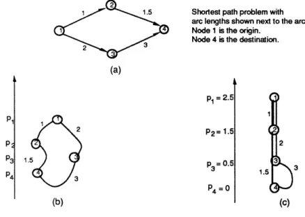
There is an interesting interpretation of the CS conditions in terms of a mechanical model [Min57]. Think of each node as a ball, and for every arc (i, j) E A, connect i and j with a string of length aij. (This requires that aij = aji > 0, which we assume for the sake of the interpretation.) Let the resulting balls-and-strings model be at an arbitrary position in three-dimensional space, and let pi be the vertical coordinate of node

i. Then the CS condition p, - pj < a,j clearly holds for all arcs (i,j), as illustrated in Fig. 5(b). If the

model is picked up and left to hang from the origin node (by gravity - strings that are tight are perfectly vertical), then for all the tight strings (i,j) we have p, - pj = aij, so any tight chain of strings corresponds to a shortest path between the endnodes of the chain, as illustrated in Fig. 5(c). In particular, the length of the tight chain connecting the origin node 1 to any other node i is pi - pi and is also equal to the shortest distance from 1 to i. (This result is essentially the well-known min path/max tension theorem; see e.g. [Roc84], [Ber91la].)

51 @ 1.5 Shortest path problem with arc lengths shown next to the arcs. Node 1 is the origin.

Node 4 is the destination. 2 If (a) pi =2.5 P2= 1.5

~~~~~~~~~~~~p

Figure 5: Illustration of the CS conditions for the shortest path problem. If each node is a ball, and for every arc (i, j) E A, nodes i and j are connected with a string of length ai, the vertical coordinates pi of the nodes satisfy pi - pj < aij, as shown in (b) for the problem given in (a). If the model is picked up and left to hang from the origin node 1, then P1 - p, gives the shortest distance to each node i, as shown in (c).

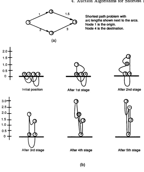
The auction/shortest path algorithm can also be interpreted in terms of the balls-and-strings model; it can be viewed as a process whereby nodes are raised in stages as illustrated in Fig. 6. Initially all nodes are resting on a flat surface. At each stage, we raise the last node in a tight chain that starts at the origin to the level at which at least one more string becomes tight.

When there is a single origin and multiple destinations, the algorithm can be applied with virtually no change. We simply stop the algorithm when all destinations have become the terminal node of the path P

4. Auction Algorithms for Shortest Path Problems

Shortest path problem with arc lengths shown next to the arcs.

Node 1 is the origin. /

3 Node 4 is the destination. (a)

2.0--1.5 1.0-0.5j

Initial position After 1st stage After 2nd stage

3.0 2.5 ₁ 2.0 1.5 1.0 0.5

After 3rd stage After 4th stage After 5th stage

(b)

Figure 6: Illustration of the auction/shortest path algorithm in terms of the balls-and-strings model for the problem shown in (a). The model initially rests on a flat surface, and various balls are then raised in stages. At each stage we raise a single ball i # t (marked by gray), which is at a lower level than the origin 1 and can be reached from 1 through a sequence of tight strings; i should not have any tight string connecting it to another ball, which is at a lower level, that is, i should be the last ball in a tight chain hanging from 1. (If 1 does not have any tight string connecting it to another ball, which is at a lower level, we use i = 1.) We then raise i to the first level at which one of the strings connecting it to a ball at a lower level becomes tight. Each stage corresponds to a contraction. The ball i, which is being raised, corresponds to the terminal node of the path.

at least once. We also note that the algorithm can be similarly applied to a problem with multiple origins and a single destination, by first reversing the roles of origins and destinations, and the direction of each arc.

The Reverse Algorithm

There are a number of ways to speed up the basic algorithm, which are described in detail in [Ber91a], [Ber91lb], and [BPS92]; see also Section 10. The most significant of these relates to a two-sided version of the algorithm that maintains, in addition to the path P, another path R that ends at the destination. To understand this version, we first note that in shortest path problems, one can exchange the role of origins

4. Auction Algorithms for Shortest Path Problems and destinations by reversing the direction of all arcs. It is therefore possible to use a destination-oriented version of our algorithm that maintains a path R that ends at the destination and changes at each iteration by means of a contraction or an extension. This algorithm, called the reverse algorithm, is mathematically equivalent to the earlier forward algorithm, and parallels the reverse auction algorithm for the assignment problem discussed in the previous section.

Initially, in the reverse algorithm, R is any path ending at the destination, and p is any price vector satisfying the CS conditions (22) together with R; for example,

R= (t), pi

=O,

if all arc lengths are nonnegative.

Typical Iteration of the Reverse Algorithm

Let j be the starting node of R. If

pj > max {p, - aij },

(ij)EA go to Step 1; else go to Step 2.

Step 1: (Contract path) Set

pi := max {pi - a j},

(ij)EA

and if i $ t, contract R, (that is, delete the starting node j of R). Go to the next iteration.

Step 2: (Extend path) Extend R by node j., (that is, make j, the starting node of R, preceding j), where

j3 = arg max {pi- a, }.

(ij)E.

If j3 is the origin 1, stop; R is the desired shortest path. Otherwise, go to the next iteration.

The reverse algorithm is most helpful when it is combined with the forward algorithm. In a combined algorithm, initially we have a price vector p, and two paths P and R, satisfying CS together with p, where

P starts at the origin and R ends at the destination. The paths P and R are extended and contracted

according to the rules of the forward and the reverse algorithms, respectively, and the combined algorithm terminates when P and R have a common node. Both P and R satisfy CS together with p throughout the algorithm, so when P and R meet, say at node i, the composite path consisting of the portion of P from 1 to i followed by the portion of R from i to t will be shortest.

Combined Forward/Reverse Auction/Shortest Path Algorithm

Step 1: (Run forward algorithm) Execute several iterations of the forward algorithm (subject to the termi-nation condition), at least one of which leads to an increase of the origin price pi. Go to Step 2.

Step 2: (Run reverse algorithm) Execute several iterations of the reverse algorithm (subject to the termination condition), at least one of which leads to a decrease of the destination price pi. Go to Step 1.

The combined forward/reverse algorithm can also be interpreted in terms of the balls-and-strings model of Fig. 5. Again, all nodes are resting initially on a flat surface. When the forward part of the algorithm is

4. Auction Algorithms for Shortest Path Problems used, we raise nodes in stages as illustrated in Fig. 6. When the reverse part of the algorithm is used, we

lower nodes in stages; at each stage, we lower the top node in a tight chain that ends at the destination to

the level at which at least one more string becomes tight.

Note that the case of multiple destinations can be handled by using a separate reverse path for each destination. One then alternates between a forward step and a reverse step as in the preceding algorithm, while taking up cyclically different destinations in different reverse steps.

Based on experiments with randomly generated problems on a serial machine [Ber91lb], the combined for-ward/reverse auction/shortest path algorithm outperforms substantially its closest competitors for problems with few destinations and a single origin (the computation time is reduced often by an order of magnitude or more). For the case of many (or all) destinations, the algorithm apparently runs slower than state-of-the-art label setting and label correcting methods (typical slowdown factors are of the order of two or three). On the other hand, for the case of multiple destinations, the algorithm is better suited for parallel computation than other shortest path algorithms. Also there is a variation of the algorithm and has substantially improved

performance for problems with many destinations. This variation is described next.

The Auction Algorithm with Graph Reduction

Despite its excellent practical performance for problems with few destinations, the auction algorithm has pseudopolynomial complexity; for an example see [Ber91la] and [Ber91lb]. Weakly polynomial versions of the algorithm were developed in [Ber9lb] using the idea of scaling the arc lengths, but these versions did not prove effective in practice. Strongly polynomial versions of the algorithm were obtained by Pallottino and

m1 ScutellOPaS91] by adding to the extension and contraction operations a reduction operation. Here, each

time a node becomes the terminal node of the path for the first time, all its incoming arcs except the one of the path are deleted, since they cannot be used to improve the distance to the node. The auction algorithm thus obtained can be shown to have an O(m2) running time, where m is the number of arcs. By using the

idea of presorting the outgoing arcs of each node in order of increasing length, the running time is reduced further to O(mn), where n is the number of nodes.

An additional advantage of graph reduction is that it allows the relaxation of the positivity assumption on all cycle lengths to nonnegativity. The reason for requiring positive cycle lengths was to ensure that no cycle could be formed through the process of path extension. On the other hand, with graph reduction, every node already visited by the path has a unique (undeleted) incoming arc except for node 1, which has no incoming arc at all. With a little thought, it can be seen that this precludes the extension of the path to a node that is already on the path.

In subsequent work by Bertsekas, Pallottino, and ScutellkBPS92] the graph reduction idea was strength-ened by using certain upper bounds to the node shortest distances to delete arcs more effectively. Two algorithms were developed. The first maintains the basic simplicity of the auction algorithm given earlier, and has O(n min{m, n log n}) running time. The second algorithm is somewhat more complex but has an

O(n2) running time. These theoretical improvements, in conjunction with efficient implementation

tech-niques, have resulted in substantially faster practical performance for single origin/all destination problems. In particular, for fully dense randomly generated problems, the auction algorithm with graph reduction has outpeformed its closest competitors [BPS92].