MITLibraries
Document Services Room 14-0551 77 Massachusetts Avenue Cambridge, MA 02139 Ph: 617.253.5668 Fax: 617.253.1690 Email: [email protected]http: //libraries. mit. edu/docs
DISCLAIMER OF QUALITY
Due to the condition of the original material, there are unavoidable
flaws in this reproduction. We have made every effort possible to
provide you with the best copy available. If you are dissatisfied with
this product and find it unusable, please contact Document Services as
soon as possible.
Thank you.
Some pages in
the original
document contain color
Constraining the QSO Luminosity Function Using Gravitational
Lensing Statistics
by
Onsi Joe Fakhouri
Submitted to the Department of Physics
in partial fulfillment of the requirements for the degree of
Bachelor of Science in Physics
at the
MASSACHUSETTS INSTITUTE OF TECHNOLOGY
May 2004
ho r
o '-;©
Onsi Joe Fakhouri, MMIV. All rights reserved.
The author hereby grants to MIT permission to reproduce and distribute publicly paper
and electronic copies of this thesis document in whole or in part.
A u th o r
...
. ...
...
...
: ...
Department of Physics
May 7th, 2004
Certified
by... ...- ...
Scott Burles
Assistant Professor
Thesis Supervisor
Accepted
by...
Professor David E. Pritchard
Senior Thesis Coordinator, Department of Physics
MASSACHUSETT
I-fSfTTE
OF TECHNOLOGY i . ,, i __ JUL 0 7 2004'--I
ARCHIVES,
,, iConstraining the QSO Luminosity Function Using Gravitational Lensing
Statistics
by
Onsi Joe Fakhouri
Submitted to the Department of Physics on May 7th, 2004, in partial fulfillment of the
requirements for the degree of Bachelor of Science in Physics
Abstract
In this thesis we use gravitational lensing statistics to constrain the QSO luminosity function at a variety of redshifts. We present a theoretical discussion of gravitational lensing statistics and illustrate how high resolution QSO imagery can be used to constrain the QSO luminosity function. We then discuss the selection and observation of the 1073 QSO exposures in our sample. The sample covers a redshift range of 0.7<z<5.5 and may include up to 10 multiply imaged QSOs. We discuss the QSO analysis pipeline developed to compute the gravitational lensing probabilities of each QSO and then present the constraints on the QSO luminosity function and compare them to results in the literature. Our results confirm the suspected fall off in the high-end QSO luminosity function slope at high redshift and agree with modern literature results. We conclude with a brief discussion of improvements that can be made to our analysis process.
Thesis Supervisor: Scott Burles Title: Assistant Professor
Contents
1 Introduction and Structure
2 QSOs
2.1 A Brief History ...
2.2 The QSO Luminosity Function .... 2.3 Cosmology. ...
3 Gravitational Lensing
3.1 Gravitational Lensing and QSOs ... 3.2 The Gravitational Lensing Setup ... 3.3 The SIS Model ...
3.4 The Lens Population ...
3.4.1 An Empirically Determined Local Lens Distribution ... 3.4.2 Simulated Redshift Dependence ...
3.5 Multiple Imaging Cross Section ... 3.6 Lensing Likelihoods ...
3.6.1 The Magnification Probability Distribution ...
3.6.2 The QSO LF as a Weighting Function ... 3.6.3 The Multiply Imaged Likelihood ... 3.6.4 The Singly Imaged Likelihood ... 3.7 Lensing Probabilities ...
3.8 Detection Probabilities ... 3.9 Constraining the QSO LF ...
4 QSO Observations
4.1 QSO Selection. ...
4.2 Instrumentation
...
5 The QSO Analysis Pipeline
5.1 Quantifying Lensing Through 2 Fitting 5.2 The QSO Analysis Pipeline ...
13 15
...
...
15
...
...
16
. . . 16 19 19 20 21 22 23 24 25 31 31 32 33 34 34 35 36 39....
39
....
40
43....
43
....
44
. . . . . . . . . . . . . . . . . . . . . . . . . . . . . . . . . . . . . . ....
...
5.2.1 5.2.2 5.2.3 5.2.4 5.2.5 5.2.6 5.2.7 5.2.8
Notation
...
Preparing the Exposure ....
Target Identification ...
The x
2Statistic ...
X
2Fitting ...
5.2.5.1 Misleading Amoeba 5.2.5.2 Signal to Noise Issues Non Lensed Simulations .... Detection Hull ... Computing Lqso ...
6 Results
6.1 mQSOs in the QSO Sample ... 6.1.1 The mQSOs ... 6.1.2 The False Positives ... 6.2 QSO LF Constraints ... 6.3 Potential Improvements ... 6.4 Acknowledgements ...
A
RFitting
Functions
B Renormalizing dPC Software Screenshots
44 45 45 46 47 48 49 50 52 54 57 57 59 65 68 70 70 73 77 81 . . . ....
...
...
...
...
...
...
...
...
...
...
...
...
...
...
List of Figures
2-1
The QSO Luminosity Function for Oh = 5.5, L. = 1010 (top, red) and 3h = 3.4, L. = 1084 (bottom,blue). /l = 1.64 for both QSO LFs ... . 17
3-1 The definition of Angular-Diameter distance, D ... 20
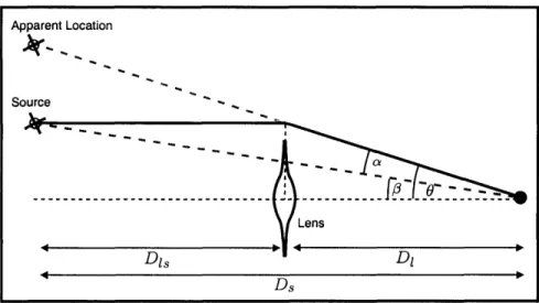
3-2 A typical gravitational lensing setup ... . 21
3-3 Left: A plot of zf vs z for M [109, 010°,1011,1012,1013,1014,1015] MG (top to bottom). The thick black line is zf = z. Right: A plot of a vs M for z E [0,1, 2, 3, 4, 5, 6] (bottom to top) . . . . 25
3-4
Left: R- the points are from the data generated by the simulation software, the contour lines are on the fitted mesh. Note that the visible points are slightly above the mesh, and that there are points slightly below the mesh that can't be seen. Right: The relative error (t f i - R) /R -. ·26
3-5
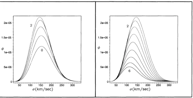
0 (number density per comoving volume (Mpc3) per a interval) as defined in equation 3.16 . .. .26
3-6 4 (number density per comoving volume (Mpc3) per a interval) presented in two dimensions. Left: 0 < z < 2 bottom to top. Right: 2 < z < 6 top to bottom ... .
27
3-7
dr vs a(km/sec) and z for (clockwise from topleft) z E [1, 2, 3, 4, 5, 6] . . . .28
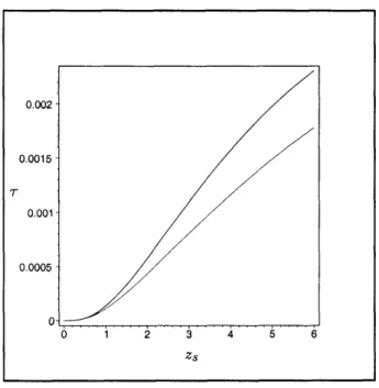
3-8 r (zs) as a function of zs. The blue (top) curve takes into account the simulated redshift evolution. The red (bottom) curve does not ... .
29
3-9 d (O, z, z,) as a function of AO and z for (from left to right) z E [1, 3, 6] . . . 30
3-10 P (O, zs) for (from top to bottom)
z
E [1, 3, 6] . . . .. 303-11
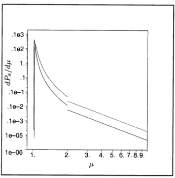
%P. dju for 0, 0.1 (red curve, top) and 0e 0.05 (blue curve, bottom) ... .32
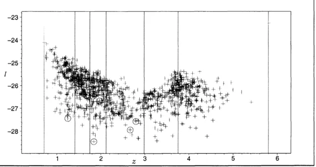
4-1 The distribution of QSOs in our sample, presented as observed absolute magnitude I vs redshift z. The blue crosses are QSOs obtained in the first run. The green crosses were obtained in the second run. The red circles denote potential mQSOs and the vertical lines delineate the redshift bins used to constrain the QSO LF ... 41
5-1 QSO Exposure 011011.243. The flux ratio between the two PSFs is 27! . ... 49
5-2 Two screenshots illustrating the difference between fit equation 5.9 (top) and equation 5.11 (bottom). In the top image, noisy sky rescaling washes out the fainter images residue (center image). In the lower image the dashed grey line delineates the boundary between A and the rest of the frame. The fainter image's residue is now clearly visible and the x2 is much higher. Finally, notice that the faint image is not visible in the QSO image (leftmost images) - this is because of the color scaling and the extreme flux ratio between both images ... 51
5-3 The Gumbel distribution overlaid on the Xv Q distribution (left) and the x2 distribution (right) for
two randomly chosen exposures ...
5-4 X2(frAL) for (from left to right) exposures 70,31, and 020101.55. The blue planes indicate the
measured value of X.2, the green planes are the threshold X.2 obtained by non-lensed simulation.
Exposures 70 and 31 are not lensed and illustrate typical variations of the shape of X* (fr, A).
Exposure 020101.55 is a potential mQSO. Note that AO is in units of pixels, not arcseconds...
5-5
Various examples of detection hulls (top) and the approximation used to compute Pmd (bottom).Each red and blue rectangle is integrated over.
011229.104, and 011231.110 . ... Exposure 117 .... Exposure 153 .... Exposure 116 .... Exposure 011011.243 Exposure 011228.48 . Exposure 011229.168 Exposure 011230.180 Exposure 011230.318 Exposure 011231.160 Exposure 020101.55 . Exposure 4 ... Exposure 287 .... Exposure 011011.170 Exposure 011011.204 Exposure 011011.241
These detection hulls are for exposures 315,
... . . . .. . 55
...
...
...
59
. . . ... . . . ... 60 . . . ... . . . 60... . . . ... . . . ... 61 ... . . . ... . . . 61 . . . ... . . . 62... . . . ... . . . ... 62 ~~~. . . . ... 63 . . . ... . . . 63. ... ... . . . ... . . . 64 . . . .. . . . ... . . . ... 65 ... . . . ... . . . 65 . . . ... . . . 66... ... . . . ... . . . 67 ... . . . ... . . . 676-16 The QSO LF Constraints. Top (left to right): the constraints in bins 1,2,3. Bottom (left to right): the constraints in bins 4,5,6. The vertical axes are h while the horizontal axes are M. The plot
beneath the curves is the color scaling used to generate the QSO LF constraint plots. The horizontal
axis is P as defined in equation 3.54. The constraints from [Pei] are presented in red, the constraints from [Madau et. al.] are presented in green, the constraints from [Wyithe and Loeb] are presented
in blue (with /h evolution) and black (without Oh evolution). Finally, the high redshift constraint
on h by [yithe] is bounded by the dashed white lines ...
6-17 The conservative QSO LF constraints, computed assuming only the verified mQSOs are, in fact, real mQSOs . ...
A-1 Plots of the fli (left) and fh, (right) fits . ...
A-2 The bi scatter plots with associated fit functions. From left to right: b,b2, and b3. ...
B-1 dPI as normalized for 01 = 0.048 and 02 = 0.079 ... .
B-2 The QSO LF constraints computed with ddA . . . . . . . . . . . . . . . . . . . . . . . . . . .
53 54 6-1 6-2 6-3 6-4 6-5 6-6 6-7 6-8 6-9 6-10 6-11 6-12 6-13 6-14 6-15 71 72 74 76 78 79
B-3 The difference P - P, as computed in each redshift bin ... 79
B-4 The conservative QSO LF constraints computed with dp dA . . . . . . . . . . . . . . . . . . . . . 80
C-1 The Coordinator ... 82
C-2 A PSF fit in the Analyzer (exposure ID: 20). The three images in the top right corner are (from top
to bottom) the selected target, the residue obtained by subtracting the target from the generated PSF, and the generated PSF. The resulting best fit parameters are presented in the lower right corner alongside the reduced x2of the fit . ... ... . 83
C-3 An example of masking in the Analyzer ... 83 C-4 The Analyzer's Xv fitting interface ... 84
List of Tables
2.1 Relevant WMAP Cosmological Parameters, the "Assumed Value" column presents values adopted throughout this thesis . ...
5.1 PSF fitting parameters (see equations 5.2 and 5.3) ... 6.1 The vital statistics of the detected mQSOs ...
6.2 The distribution of QSOs and mQSOs in the LF constraint bins. ...
A.1 The fit parameters for fhand fj ... A.2 The parameters for the bi functions . ...
the parameter . . . .. . 17 . . . 46 ... . . .. . 58 ... . . . 68 ... . . . 74 ... . . .. . 75
Chapter
1
Introduction and Structure
This thesis represents the culmination of two and a half years of research under the guidance of Professor Scott Burles in the MIT Physics department. In it, we shall detail a holistic approach to the problem of constraining high redshift QSO statistics using gravitational lensing probabilities. Our approach incorporates several interrelated theoretical, observational, and computational elements and we shall not attempt to describe them in this brief introduction. Rather, we shall motivate and connect the different elements together throughout the thesis.
We will, instead, present a quick overview of the thesis' structure:
Chapter 2 presents a brief history of QSOs, describes the QSO Luminosity Function, and offers
motivation for the thesis' ultimate goal: constraining the QSO Luminosity Function.
Chapter 3 describes gravitational lensing theoretically. In it we present the Singular Isothermal
Sphere (SIS) gravitational lens model and derive the distribution for the gravitational lens popu-lation. We then present derivations of the lensing probability equations and describe the means by which high resolution QSO imagery can be used to compute the lensing probabilities. We end the chapter by describing how the lensing probability equations can be used to constrain the QSO Luminosity Function.
Chapter 4 describes the selection criteria used to select the 1073 QSOs in our high resolution
QSO sample. It also discusses the instrumentation used to obtain the imagery.
Chapter 5 describes the QSO analysis pipeline. It motivates and presents the 2 statistic
and describes, in detail, the fitting procedure used to compare objects within exposures to identify lensed QSOs. It then describes the simulation techniques used to quantify the empirical lensing probabilities and the limitations of our technique's lens detection capabilities.
Chapter 6 concludes by presenting the results of the analysis process. It includes a
presen-tation of the identified lensed QSOs in our sample, and the resulting QSO Luminosity Function constraints. The chapter ends with a discussion of the limitations of our approach and offers po-tential improvements to the theoretical and computational techniques we have used.
The thesis also contains three appendices. The first of these presents an analytical fit to the lens distribution derived in chapter 3. The second describes an alternate normalization of one of the theoretical probabilities derived in chapter 3. The motivation for this renormalization will be
explained in that chapter. The third appendix presents some screenshots and a brief description of the Coordinator and the Analyzer, two software packages written to organize and analyze the QSO sample.
Chapter 2
QSOs
2.1
A Brief History
The 1940s and 50s saw a boom in radio astronomy. With the development of new technologies and, more importantly, the growing academic interest in radio astronomy, the number of known radio-loud objects in the universe began to grow rapidly. The new radio observations were carried out hand in hand with complimentary optical follow ups of the radio-loud objects; more often than not, the radio sources were identified optically as galaxies.
In 1960, however, things changed when Thomas Mathews and Allan Sandage went in search for an optical counterpart to radio source 3C48, an uncharacteristically small radio source, less than an arc-second in diameter [Thorne]. Using the 5-meter Palomar optical telescope, Sandage was surprised to find a single, star-like, blue point at the radio source's coordinates. Sandage recalls, "I took a spectrum the next night and it was the weirdest spectrum I'd ever seen." [Thorne]
It would only be a few months before the Dutch astronomer Maarten Schmidt would recognize the heavily redshifted Hydrogen Balmer lines in the spectra of these newly-christened Quasi Stellar
Radio Sources (quasars). According to Hubble's law these objects, which appear to be moving
away from the Earth at relativistic speeds, must be extremely far away and, by virtue of the fact that they can be observed today, must be exceedingly bright. In fact, quasars can be up to 105 times more luminous than normal galaxies [Carroll]. While there is no direct evidence, most astrophysicists are convinced that these objects must be driven by large black holes in their cores; quasars are probably extreme examples of Active Galactic Nuclei (AGNs).
Optical astronomers quickly began actively searching for quasars and it was soon discovered that only about 10% [Carroll] of the spectroscopically confirmed quasars they found were radio-loud. Thus, "quasar" is a misnomer and these point-like high redshift objects are now referred to as
Quasi-Stellar Objects or QSOs. Recent surveys, such as the Sloan Digital Sky Survey (SDSS),
have led to an exponential growth in the number of known QSOs. According to [Carroll] there were about 5000 QSOs known in 1996. Today, SDSS alone reports 32,241 QSOs with redshift < 2.3 and 3,791 QSOs with redshift > 2.3 [SDSS]!
2.2 The QSO Luminosity Function
The fact that QSOs are extremely far away and extremely bright makes them excellent probes of the early universe: By understanding the distribution of QSOs we can test the assumption of isotropy and homogeneity in the universe, attempt to understand the underlying physics behind the evolution of QSOs with redshift, and constrain the black hole accretion models that attempt to describe QSOs [Pei].
The most commonly used QSO distribution is the QSO Luminosity Function (QSO LF). We define the QSO LF, (L, z) dL, as the number density (per comoving volume) of QSOs at redshift z with luminosity L < lqso < L + dL. The commonly accepted empirical model for the QSO LF at z < 2.2 is a double power law shaped LF [Boyle et. al.]
'h(z)
T
'()
21
( L )10
+ ( L )h
(2.1)
Here, 0 (z) is a redshift dependent overall normalization that has units of number density (per
comoving volume) per luminosity and L, (z) is referred to as the break luminosity; it parameterizes the kink observed in the QSO distributions and also depends on redshift (see figure 2 in [Pei]). I and Oh are, respectively, the low end (below the kink, towards low luminosities) and high end (above
the kink, towards high luminosities) slopes of the QSO LF with
f
< ph. These parameters mayalso depend on redshift, though a quick look through the literature [Comerford et. al.], indicates that most authors ignore such dependences, even at high redshifts. The literature also points to a fair degree of disagreement regarding the evolution of Lwith redshift [Comerford et. al.].
The QSO parameters are generally obtained by fitting equation 2.1 to an observed QSO distribu-tion. We shall take a different approach; our goal, in this thesis, is to constrain the L, and Oh QSO LF parameters at a variety of redshifts using gravitational lensing statistics. We will compare our constraints with the best-fit estimates of [Pei], [Madau et. al.], and [Wyithe and Loeb] as tabulated by [Comerford et. al.]. Figure 2-1 presents two representative normalized QSO LFs.
2.3
Cosmology
Perhaps it is now appropriate to discuss the assumptions regarding cosmology that will be made throughout this thesis. Some authors (notably [Mitchell]) have used QSO gravitational lensing statistics to constrain cosmology. While this is certainly an excellent use of QSO lensing statistics that offers independent verification of the values of cosmological parameters, the accurate results of WMAP set far stronger and more robust limits on cosmology. Thus, in this thesis, we will assume the most recent cosmological parameters, as observed by WMAP [Bennett et. al.] (see table 2.1) and will choose to concentrate our use of gravitational lensing statistics to better constrain the QSO
.1
Figure 2-1: The QSO Luminosity Function for h =
blue). Al = 1.64 for both QSO LFs.
Parameter
5.5, L, = 1010 (top, red) and 3h = 3.4, L,, = 1084 (bottom,
Value Assumed Value Q- Total density
QA- Dark energy density Ql- Matter density
Qk- Curvature (effective) density
h - Hubble constant
as - Fluctuation amplitude in 8h- 1 Mpc Spheres
1.02 i 0.02 0.73 ± 0.04 0.27 ± 0.04 0 0.71 (+0.04,-0.03) 0.84 ± 0.04
Table 2.1: Relevant WMAP Cosmological Parameters, the "Assumed Value" column presents the parameter values
adopted throughout this thesis.
.1 0 Q .1 .le log(L) 1 0.7 0.3 0 0.71 0.84
Chapter 3
Gravitational Lensing
3.1
Gravitational Lensing and QSOs
That gravity should affect the trajectories of photons is not a new idea. As early as 1783, by treating "corpuscles" of light as particles with velocity c, John Michell showed using Newton's
theory of gravitation that a star could conceivably be sufficiently compact that no light corpuscles could escape to infinity. It would be impossible for observers to see such a "dark star" [Thorne]. Today we have Einstein's formulation of the General Theory of Relativity to guide our calculations and, while the modern day black hole is fundamentally different from Michell's "dark star," the essential idea behind both phenomena is the same: gravity bends light.
In 1919 the English physicist Sir Oliver Lodge proposed that light could be focused by massive bodies in a manner similar to the focusing effects of optical lenses. This phenomenon is called
gravitational lensing, and the massive body that causes light to bend is called a gravitational lens. While all massive bodies can act as gravitational lenses, Fritz Zwicky proposed in 1937 that
the majority of observable gravitational lenses would be galaxies [Carroll].
In order to observe a lensing event it is necessary to place the lens between a light source and the observer (in our case, the Earth); as QSOs are both far away and bright, one would expect the chances of observing a QSO lensed by a galaxy to exceed the chances of observing other lensed objects. For this reason, QSOs have become popular targets in the search for gravitational lensing phenomena.
In the next few sections in this chapter we will discuss the population of gravitational lenses that are most likely to ]lens QSOs. We will describe the distribution of these gravitational lenses and use these distributions, along with the QSO LF, to compute lensing probabilities. We will then show how the resulting probabilities can be applied to observational data to set constraints on the QSO LF. To proceed, however, we will first need to understand the conditions under which gravitational lensing occurs, and choose an analytical model to describe the lensing phenomenon quantitatively.
Figure 3-1: The definition of Angular-Diameter distance, D.
3.2 The Gravitational Lensing Setup
We will be studying systems involving cosmological distances but there are several different distance measures in cosmology [Hogg]. In geometries relevant to gravitational lensing systems, however, the most useful distance measure is the angular-diameter distance: Given two objects at the same
redshift 2 separated by a small angle 0 on the sky as seen by an observer at z, we define the angular-diameter distance between the observer and the objects to be D such that
x
D
(3.1)
where x is the physical separation between the two objects (see figure 3-1). To compute the angular-diameter distance between two objects at redshifts zand 2 > Z1 we use
D
=
DM
(2)
- DM ()
(3.2)
D = (3.2)
1 +Z2
where DM (z) is the comoving distance given by
Z
dz'
DM (z) =
DHE(z')
(3.3)
with E (z) given by
E (z) =
V/QM
(1
+
z) + A
(3.4)
and DH = 3000h--lMpc is the Hubble distance. These equations are taken from [Hogg] and have been simplified by assuming that Qk = 0.
Now, consider the setup in figure 3-2. The distances Dl, D, and Dis are the angular-diameter distances between the observer and the lens, the observer and the source, and the lens and the source respectively. The lensing equation [Narayan and Bartelmann], in terms of the parameters in
figure 3-2, is simply
- a () . (3.5)
To compute a we need the surface-mass distribution E of the lens (assumed to be thin and well
Z2
t ::
Apparent Location Source X_ -q I --- -- -- -- -- - -- -- -- -- -- -- -- -- -- - -- - -- -- -- - -Lens
Ds
D
DsFigure 3-2: A typical gravitational lensing setup.
localized at a single redshift). If we assume a circularly symmetric mass distribution Z (r) then it can be shown that; (see [Narayan and Bartelmann])
D1 4 I
= 20 [ j2D1
E (r) rdr.
(3.6)
DID c6
The integral is simply the lens mass enclosed by a circle of radius DIO. To proceed we'll need to select an appropriate surface-mass distribution; the most commonly used distribution is the SIS model which we discuss next.
3.3
The SIS Model
Gravitational lenses bend light gravitationally, not optically. While the refractive properties of an optical lens depend on the material and geometry of the lens, the refractive properties of gravi-tational lenses depend on the distribution of mass in the lens plane. In statistical applications of lensing the most commonly used mass distribution is the Singularly Isothermal Sphere mass
profile (SIS) as it yields simple, analytical, expressions that can be easily incorporated into prob-ability computations while offering a good approximation to actual mass distributions observed in galaxies.
The SIS model is not parameterized in terms of the total galactic mass, as one might expect. Rather, since most of the mass in galactic halos is due to dark matter, which astronomers cannot observe directly, it is more convenient to use a, the velocity dispersion. By definition, a is the one dimensional velocity dispersion of the stars in the galactic halo and, since the stars are influenced
'[Li and Ostriker] disagree with this statement, they claim an NFW profile (first described by Navarro, Frenk &
gravitationally by both luminous and dark matter, a is a measure of the total mass density profile of the galaxy.
The SIS model treats the mass components in the galactic halo like ideal gas particles under the influence of their own spherically symmetric gravitational potential. A simple thermodynamic derivation, relating temperature to a, (see [Narayan and Bartelmann]) then yields the SIS surface-mass density
02i
Z (r) = 2G
1
(3.7)2Gr
This mass distribution, when coupled with equation 3.6, yields 0'2 D1 8s
a
=
4r
2D -E
(3.8)OE
where E is the Einstein radius of the lens. Note that OE is independent of
:
but does dependon the distances (and therefore redshifts) of the lens and source. The lensing equation yields two solutions for
0,
the observed position of the source, if:
< OE (see [Narayan and Bartelmann])O+ = ±OE-
(3.9)
In this regime the source is said to be strongly lensed: the lens both magnifies the source and pro-duces multiple images. We can compute the separation AO and magnification ,± [Narayan and Bartelmann] of these two images to find
AO
=
+
-_ = 20E
(3.10)
O+ OE
1+ =
-=1
(3.11)
If > SE then we only observe one image at a position 6+ with magnification
p+
and the source is said to be weakly lensed. Weak lensing is very hard to identify in observational data.Combining these results we can compute the total magnification of the source
{ X-A_ P 2oE for/ < E(
~
(/3)
=
+
for-3•6-
(3.12)
1
+~
OEfor/>
OE
The separation AO (a) and magnification (,, 0a) are the only two results we will need from the SIS model.
3.4
The Lens Population
We now have a gravitational lens model, the SIS model, determined completely by the redshifts of the source and lens and the velocity dispersion of the lens. The next step towards computing lensing probabilities involves understanding the distribution of the lens population. Ideally, we would like
to have at our disposal a lens distribution, 0, of the form
n (a', z) = (', z) da (3.13) where n is the number of lenses per comoving volume with velocity dispersion a' - d < a < a' + at redshift z for vanishingly small da.
A wide variety of objects might contribute to the lens distribution and examples vary from the extreme, such as cosmic string loops [A de Laix et. al.], to the ordinary late-type and early-type galaxies. In our discussion we shall follow [Mitchell] and focus on the dominant contributions made by early-type galaxies.
Most lensing statistics studies compute the lens distribution using an empirically determined early-type galaxy luminosity function combined with the Faber-Jackson relationship, which relates luminosity to the velocity dispersion . [Wyithe] points out, however, that this approach is un-reliable as it ignores the intrinsic scatter in the Faber-Jackson relationship. Also, this approach generally ignores the evolution of the lensing population with redshift. We will present an alterna-tive technique for obtaining 0, based on [Mitchell], in the remainder of this section.
3.4.1
An Empirically Determined Local Lens Distribution
Recently, [Sheth et. al.] fit a modified version of the Press-Schechter ([PS]) mass function of dark matter haloes (first presented in [Sheth and Tormen]) to SDSS velocity dispersion data. They obtained an empirical fit to the distribution of among 30,000 local (z 0) early-type galaxies given analytically by
01
a 011/
du
ST()
dci=q (
)
[*exp
-
]
(3.14)
or*
a*
F (a//3)ci
with 0* = (1.4 ± 0.1) x 10-3Mpc -1a* = 88.8
±
17.7km/sec
a
= 6.5
i±1.0
,/
= 1.93
±
0.22
The Sheth-Tormen distribution is only valid at z = 0 and one would expect that (, z) should
evolve with redshift. This is due to the fact that dark matter haloes merge, and that the velocity dispersion of the resulting halo generally exceeds the velocity dispersions of either constituent halo. Thus, we would expect the number of high haloes to decrease with redshift.
There is little empirical data describing the evolution of kST () with redshift. Several authors (e.g. [Wyithe]) assume a simple independent redshift evolution of the lens distribution; [Mitchell], however, makes use of N-body galaxy formation simulations to produce a fully a-dependent redshift
evolution. We shall do the same.
3.4.2
Simulated Redshift Dependence
Our approach will be to use N-body simulation results to compute the ratio
OR (, Z) =- N (, Z)
(3.15)
ON'(o, 0)
where, N is the lens distribution computed by the simulations; in this equation N stands for
N-body simulation while R stands for ratio. We will then combine this theoretical result with Sheth's [Sheth et. al.] empirical ST (, z = 0) lens distribution by defining
(
(a,z) 'ST (a) OR (a, z).(3.16)
The N-body simulations used to compute R (,z) were performed by [Jenkins]. Professor Jenkins has graciously provided us with software that returns the computer simulation results for different cosmological models. The software takes several input parameters which we briefly describe
now.
The first set of parameters specify the simulated universe's cosmology; we set
Qm
= 0.3 and QA = 0.7. The software also requires a power spectrum. The power spectrum describes the initial distribution of perturbations in the universe; these perturbations eventually collapse into galaxies. Following [Li and Ostriker] we use the analytical power spectrum fit proposed by [Eisenstein and Hu], normalized by WMAP's value of the normalization constant: as = 0.84 (see table 2.1).Professor Jenkin's software returns the number density (per comoving volume) of galaxies at a given redshift as a function of M, the mass of the galaxy haloes: N (M, z). To proceed we must first
convert this to a function of a. [Mitchell] outlines the procedure that must be followed to relate a to M; it requires taking into account the fact that o (M) relies on the formation redshift of the halo (zf, the epoch when the halo collapsed). The formation redshift is discussed in [Lacey and Cole] where the authors obtain (essentially) the probability distribution of zf as a function of z and M. [Mitchell] simplifies the distribution by setting f to be the mean (zf) obtained from the [Lacey and Cole] distribution. [Mitchell] checks, and ensures, that ignoring the dispersion in the zf distribution does not significantly affect R (a, z). Thus, we can speak of a function f (M, z) which allows us to
define a (M, zf). All the relevant equations are available in [Mitchell], we simply present the results of this computation in figure 3-3.
We can now rescale the N (M, z) distribution to find
'N (a
(M, z), z)
= N (M,Z) d
(3.17)
Zf .5e4 .1e4 ,.5e3U Q) E ,.1 e3 b .5e2
.lez le+10 le+11 le+12 le+13 le+14 le+15
0
M(M0)
z
Figure 3-3: Left: A plot of zf vs z for M E [109, 1010, 1011, 1012, l013, 1, 1015] M® (top to bottom). The thick
black line is zf = z. Right: A plot of a vs M for z E [0,1, 2, 3, 4, 5, 6] (bottom to top).
us OR ( (M, z), z) at corresponding discrete values of a. We will soon see, however, that we need
to be capable of integrating over OR quickly. To achieve this we have put together a series of fitting functions, fit, that match the R (a, z) distribution well (see figure 3-4). We present the form of the fitting functions, with the fitting parameter values, in appendix A. The fits are valid for 20 < a < 700 and 0 < z < 6.
The relative deviations between the fit and the data are presented in figure 3-4. The high deviation in the far right quadrant is due to the fact that R is very close to zero in that region and even the slightest fit error is largely magnified. However, since R is so close to zero in that quadrant, the contributions of the errors will be quite insignificant when we ultimately use R in lensing probability computations.
Figure 3-5 presents the final distribution as obtained by combining R with ST (equation 3.16). Figure 3-6 is a two-dimensional presentation of 0 for 0 < z < 6; note the marked drop in the number of high a lenses with increasing z.
3.5
Multiple Imaging Cross Section
We have presented the SIS lens model and have obtained the redshift dependent lens distribution we were after. It is now time to combine both results to obtain multiple imaging cross sections. These cross sections are to be interpreted as the geometric probability that a point source at some redshift z is multiply imaged by a foreground lens. To be precise, we seek a function d (zs, z, a)
Figure 3-4: Left:
¢R-
the points are from the data generated by the simulation software, the contour lines are onthe fitted mesh. Note that the visible points are slightly above the mesh, and that there are points slightly below the
mesh that can't be seen. Right: The relative error (fit - NR) /'kR
Figure 3-5: ¢ (number density per comoving volume (Mpc3) per a interval) as defined in equation 3.16.
I-0 LLJ a) 2e-05 1.5e-05 1e-05 5e-06 0 6 1 Z vc v- 0
-,-
J,---s< ~ ~ ~ ~ *f2e-0
Figure 3-6: (number density per comoving volume (Mpc3) per a interval) presented in two dimensions. Left:
0 < z < 2 bottom to top. Right: 2 < z < 6 top to bottom.
such that
dT (Z,
z', ') dzdo
(3.18)is the probability that a source at redshift z is multiply imaged by lenses living in the phase space:
z'-dz
< z <
z'
+
and
a' _ d- <
<
+ . We can then define
()
j
d (s, z, a) dadz (3.19)J0 J0
to be the geometric probability that a source at redshift Zs is multiply imaged. We use the term geometric probability to emphasize the fact that the probability does not depend on any properties of the source other than its position (i.e. redshift), we will see later that we can define true a priori lensing likelihoods that take into account the luminosity of QSO sources.
The SIS model tells us that the multiple imaging cross section of a lens at redshift z, with velocity dispersion a, and lensing a source at redshift zs is given by
A(a,z,z) = r(DIOE)
2= 16r
3()
4(D
s)2
(3.20)
Ds
Now, (, z) da is the comoving number density of lenses with multiple imaging cross sections A (a, z, zs) in a dispersion velocity interval da. According to [Hogg] the incremental probability that
1.5e-0'
le-O.
5e-O
2e-06
-1.5e-06 -1 e-06 -5e-07 d'r -dT I / l 5e-06 4e-06 3e-06 2e-06 1 e-06 0 l I | l l I"
1e-05 8e-06 6e-06 4e-06 2e-06 , O 1 e-05 8e-06 6e-06 4e-06 2e-06 ,0 :7) '1~~~~~~~~~~~~~~~~~~~~~~~~~~~~~~~~~~~~~~~~~~~~~~~~~~~~~~~~~~~~~~~~~~~~~~~~~~~~~~~~~~~~~~~~~~~~ } o I1~ ~ ~ ~ ~ ~
~
eI III IFigure 3-7: dT vs (km/sec) and z for (clockwise from topleft) z E [1, 2, 3, 4, 5, 6].
a line of sight will intersect one of these objects at redshift z in a redshift interval dz is
( + Z 2
dr(zSz, ) dudz = (u, z) A (,zz)
DH
(E(z) dadz
(3.21)(refer to section 3.2 for the definitions of DHand E (z)). This is precisely the expression we are
looking for.
Figure 3-7 presents six plots for dr at source redshifts z [1, 2, 3, 4, 5, 6]. Note the behavior at large z where there is little contribution to the multiple imaging cross section beyond z 3.5, this is due primarily to the lensing geometry encapsulated in the D (z, z,) term, but is accentuated by the redshift evolution of the lens population.
Figure 3-8 presents two plots of (z,). The blue (top) curve is (z,) as defined in equation 3.19, complete with the simulated redshift evolution. The red (bottom) curve ignores redshift evolution completely. Interestingly, the redshift evolved lens population has a higher multiple imaging cross section. This can be understood by noting the formation of a peak in the lens distribution at z 2 in figure 3-5 which amplifies the multiple imaging cross section contribution by lenses at z 2. The effects of the peak are manifested in the steep slope of r (z,) at z 2.
We now perform one more refinement to our analysis and present the multiple imaging cross
8e-06 6e-06 4e-06 -2e-06 dr 04 4 I I I I | ll ll I I I ; ll~~~~~~~~~~~~~~~~~~~~~~~~~~~~~~~~~~~~~~~~~~~~~~~~
Figure 3-8: T (zs) as a function of z. The blue (top) curve takes into account the simulated redshift evolution. The red (bottom) curve does not.
section, d, as a function of the image separation AO instead of a. To do this we invert equation 3.10 to find
(AO, Z, Zs) =
.
DsAO (3.22)We then insert this expression into d (a, z, zs) and rescale the distribution by d#A (which we can compute analytically) to find:
duAO h,z,zs
dT(L/.6,zvzs)
dT(af(t6,ZZ 5),'ZZ)daO
as~z~zs(3.23)We can now use equation 3.23 to define P (AO, zs) (as in [Barkana and Loeb]), the (cumulative) probability that a lensed source at redshift Zs has an image separation > AO
roof rz
P
(AO,
zs) =
Jj dr(Ao', z, z
5) dzdA'.(3.24)
We can also define the differential probability
dP
_dO - dr (A', z, z,) dz. (3.25)
Figure 3-9 is a plot of dr (0, z, z,) for z E [1, 3, 6] and figure 3-10 is a plot of P (0) , Zs for
Zs E [1,3,6]. 0.002 0.0015 -T 0.001 0.0005 - 0-0 1 2 3 4 5 6 ZS 4 5 6
0.0014 0.0012 0.001 0.0008 0. 0006 0.0004 0.0002 0 dr l I i
iI
.00035 -0.0003 .00025 -0.0002 .00015 0.0001 5e-05 dr 0 1I
_I
I
Figure 3-9: d (AO, z, zs) as a function of AO and z for (from left to right) z E [1, 3, 6].
1- 0.8-
0.6-P.
0.4- )2-0O U 1. .1le-1 .1 Z/O( )Figure 3-10: P (AO, z,) for (from top to bottom) z E [1, 3, 6].
I .1 A, _- (} - I a, I i -* j I , I I .l
3.6
Lensing Likelihoods
We can now determine the probability that a QSO, with luminosity Lqso, is multiply imaged. This will involve taking into account the information provided by the QSO LF to weight the probability that the QSO is magnified by a factor M. For brevity, we shall refer to multiply imaged QSOs as
mQSOs.
3.6.1
The Magnification Probability Distribution
To begin we will need to determine the magnification probability distribution for a given SIS lens. We first rewrite equation 3.12 in terms of p
forip>2
/. - (3.26)
OE
for 1 +
<
<26)
Now, is an angle on the sky defined such that = 0 at the center of the lens (see figure 3-2) and the probability distribution of is given by
dP 1 1
d =
-
27rsin/o = I sin.
(3.27)
do3 4w 2
But using equation 3.26 we can compute the corresponding magnification probabilities as dlP =
|dP |
d dj
du = Esin 2E for > 2
dA A 2 A
~~~~~~~~~~~~~~(3.28)
dPU -
dA
)22(1,-
sin
(i) for1 +
<< 2
(3.28)iL_ ~~~~7r
Here d- and represent the multiple imaging and single imaging magnification probability
distributions respectively. Plots of these distributions are presented in figure 3-11.
Now, note that, the integral
f
2 d dp is the multiple imaging cross section of the lens and that it evaluates to the appropriate valuef°OE.
20E
d+
1
132
X
2sin
-
=
cos
(E)
+
(3.29)
A2 A - 2 2 4,7r
(assuming OE is small).
This result allows us to replace equation 3.20 with
A (, z, z) = rD 202 = 47rD2 E
sin
Ed
J
E 1 2Ds s= 167r2D X 2 2 sin - 2 Ds (3.30)
where we have substituted using equation 3.8. We can now substitute equation 3.30 into the where we have substituted E using equation 3.8. We can now substitute equation 3.30 into the
.1
Figure 3-11: dP- for 0e 0.1 (red curve, top) and 0e 0.05 (blue curve, bottom)
di,
expression for r (zs) (equation 3.19) to obtain an integral expression for r of the form
(1 + z)2
(Zs)
= /
dT
(z, z, a) ddz =
DHq 5
(, z) A(a,z,z
EZ)
dadz
= oE(z)o
f~s/'O~fOO(1
+z)
21
r
2DO
ls
[8
i
ru
2Djl
= 1672DH
0Jo02
D2 (, Z) ( Z) 2 2 DIs sin [- 2DI dpdudz
(3.31)
E (z)
C2 D, [p It c2 DJ This allows us to define d, (zs, z, a, t) as a function of [dT (a,z,z s,/I) = 16+r2D Dz
1 r
q (
2D
(E (z) t_
z) 2I(z)
2c
22D s
D_ sin[
c
2Ds
1.
(3.32)3.6.2
The QSO LF as a Weighting Function
We now seek to incorporate the QSO LF with the multiple imaging cross sections. If we consider an mQSO with observed magnitude iqso, and naively compute its intrinsic luminosity2 Lqso, then
the actual intrinsic luminosity of the QSO is Lqso where is the magnification due to gravitational lensing.
Assuming our QSO LF describes the intrinsic distribution of QSO luminosities, we can describe the relative likelihoods of observing a QSO at redshift z with different magnifications . All we need to do is evaluate the luminosity function (equation 2.1) at
XP
(L_ 0, zs) and the larger theresult, the more likely the QSO is magnified by . Note, however that the actual probability of finding a QSO with intrinsic luminosity L within some AL interval is I (L, zs) AL, if we replace L
2
We will discuss how this is done in section 5.2.8. .1
.le
.1e 1e-2. 3. 4. 5. 6.7.8.9. It I Duo 1.with
L=
Lgaowe must replace
Lwith some
where ALqso is a constant independent of p.This, then, allows us to write the magnification probability weight factor
p( Z s (3.33)
3.6.3
The Multiply Imaged Likelihood
We can use equation 3.33 to weight the multiple imaging cross section element, d, and define the
multiply imaged likelihood
3m (lqso°Zs)
= jd (a,
zz,)
4
(- so Z 'dLdadz.
(3.34)
This is a rather complicated triple integral and is not easily separable because the sin 8 D
term in equation 3.32 combines all three integration variables in a nonlinear fashion. We can, however, assume that S 7D_ _ 20
p cT
<D,, j,
E < 1 and write sin[
-7 D,
£- c- 87r D-~~~~~~~~c
T
D,
Equation3.6.3 then separates to give
z co
~
+ z) 2
b0o
d
8da
,z
dZ
s.
Lm
(IqsoZs)
~~qso,
~
JOO
Job
A (az z)(
E (z)J2'
) (a(z(, z) ddz
|4
(Lk.
z
8sd
du
00 8 ,~
~~~~¥I
LqsoT (Zs) j- 4 4
(Pi
8
s) d. (3.35)We can reinterpret this result to shed light on the physics of the small angle approximation. Consider a single lens with multiple imaging cross section (Zs) = 47r 4. The Einstein radius of this lens is
0 E- 2 T(z ) (3.36)
and figure 3-8 assures us that E << for all Zs < 6. The multiply imaged likelihood due to the lens is then given by
fd (Lq_
1
f20 2i
2
rn (Lqso, Zs)
=Jd
m
poZ
,zzs)d
sIdlL J
/4
E
= (Zs) -jO4 ( Lqs, zs) d. (3.37)
This is precisely the result obtained in equation 3.35. Equations 3.36 and 3.37 offer an interesting physical interpretation for the approximation in equation 3.35; the individual lenses in the lens distribution can be brought together and treated like one large lens with a total multiple imaging cross section equal to the total cross section of all the individual lenses. In a sense, we are moving the lenses from their random locations on the sky together, combining them, and treating the resulting
3The multiply imaged likelihood is not a probability distribution. It is not normalized and must be combined with
lensing mass like one large SIS lens.
3.6.4
The Singly Imaged Likelihood
This interpretation of the multiply imaged likelihood, as codified by equation 3.37, motivates the
definition of the singly imaged likelihood
1s (Lqso, Zs) = , dP (6OE, ) ( I ,LZs) 'd (3.38)
where dP- (E, ) is defined in equation 3.36, and OE is given by equation 3.28.
The relationship between Cm and Cs can be clarified by taking a step back and removing the QSO LF weight function. Then, by definition
2
dPs d/ dPm
I
ddu + / d/a = 1 (3.39)+O~ d d/
which, by equations 3.29 and 3.36, gives us
2
dP,
2
d du = 1 - r (zs)
(3.40)
i+0E dp
Thus, equation 3.38 takes into account the magnification outside the multiple imaging area of the large lens constructed through equation 3.36. This interpretation leads to an interesting problem. Equation 3.38 only incorporates magnifications with
1 < +- < < 2 (3.41)
7r
implying that every source, (whether inside or outside the multiple imaging area), is magnified. Clearly, such a situation is unphysical - by conservation of photons alone we expect that the mean magnification, (), over all sources should be unity. The SIS model does not allow for demagnifi-cation and, as such, is unrealistic far from the lens at low L, (though the approximation is quite valid for > 2 inside the multiple imaging radius). Several authors (e.g. [Comerford et. al.] and [Wyithe and Loebl) have attempted to bypass this problem by extending -dP down to < 1 and rescaling the resulting distribution to yield () = 1 while conserving the relationship in equation 3.40. We have done the same and present the resulting renormalized dp- as well as the (small) changes in the QSO LF constraints in appendix B.
3.7 Lensing Probabilities
The lensing likelihoods introduced in sections 3.6.3 and 3.6.4 are not, strictly speaking, probabilities. They have not been normalized, and doing so would be difficult as we do not understand the behavior of To (zs) (see equation 2.1) with redshift very well. To get around this we now define actual lensing
probabilities. The first is the multiply imaged probability:
P = -
.m
(3.42)
£m + s
and the second is the singly imaged probability:
Pi -LS (3.43)
£m + s
Thus, given a QSO with luminosity Lqso, the probability that it is an mQSO is Pm. Note that, while these probabilities depend on z, the redshift of the QSO, and Lqso, the observed luminosity of the QSO, there is also an implicit dependence on the parameters of the QSO LF. In particular, the probabilities may be sensitive to changes in fl (the low end QSO LF slope),
/3h(the
high end slope), and L,(the break luminosity) (see equation 2.1). By taking ratios of the lensing likelihoods, however, we have effectively canceled out the dependence on 0(zs).Of course, equations 3.42 and 3.43 satisfy
Pm+Ps = 1 (3.44)
3.8 Detection Probabilities
The multiply imaged probability, Pm, predicts whether a QSO with observed luminosity Lqso is multiply imaged or not. It does not, however, take into account the fact that we cannot identify all mQSOs. It is possible, for example, that the multiple images are too close together and, therefore, unresolved even in high resolution imagery. It is also possible that the images are fairly well separated, but that the flux ratio between the two images is too far from unity to allow for a successful detection of both images.
These two factors: the flux ratio (which we will denote fr from now on) and image separation (which, following our current notation, we denote A0), determine whether an mQSO can be resolved or not. More explicitly, if we consider the phase space (fr, AO) we can define a subset of the phase space in which mQSOs will be successfully detected. We call this subset the detection hull and shall discuss its properties, from an observational point of view, in section 5.2.7. For the current theoretical discussion, however, let us assume we are given a detection hull for a given QSO. We must now modify our definition of Lm (in equation 3.34) to take the detection hull into account.
We begin by defining fr in terms of the SIS model parameters. Combining equations 3.11 and 3.26 we can write
=1±+
2
(3.45)2
and then define
fr
=-/-=
p
2
(3.46)
Since <o 2 in the multiple imaging regime we have 0 fr 1. Equation 3.46 allows us to
define p in terms of fr
1l±fr
2
= 2 fr (3.47)
and this definition will allow us to convert the detection hull from (fr, AO) phase space to (, A
0)
phase space. With this in mind, let us reconsider equation 3.34
,m
(Zsl) Iqso) =j702
dr, (Zs,
z, a,p) (lqsoI-ddadz.
A P
Our first step will be to express the integral in terms of /AO instead of a. We've done this before,
in equation 3-9. VVe define
dr, (AO, , Zs,A ) = dr ( (AO, z,
,Zs,Z, ) dAO
(3.48)
Now, using the approximation made in equation 3.35 and the result obtained in equation 3-9 we can write d, (AO, z, z, p) as
d-r, (AO, , s, p o, z s) A [ ](,0,Z 8 , 1qo~
dz ,(Z\,Z~s,)
[A(()
zzs)
(+z)
2(
(
) z) da
O
1
(
/1)l
ILu4 ( A )]
= dT(A6,
Z,z s[44
(l-~,zs)]
.(.9
We can now define md, the likelihood that a QSO is multiply imaged and detected as such to be
£md
=
fdr(,zz)dz
[4
(AO,
,ZsdAOdpt
(3.50)
where DH is the detection hull delineated in (, AO) phase space. Note, that the integral over redshift simply yields dp as defined in equation 3.25. Thus, we obtain a simplified version for our definition of .mdmdJJ
idP (AO, s) (l
_
z
s)
dAOdp.
(3.51)
H I.4
dAO
Using Lmd we define the probability that an observed QSO is multiply imaged and detected as such to be
Prod =- Csd (3.52)
LCm + Ls'
3.9
Constraining the QSO LF
We now have all the pieces necessary to constrain the QSO LF. Consider, now, that we have at our disposal a collection of QSOs with redshifts in some redshift range z < Zs < 2 and a variety
of luminosities, Lqso. Let us also assume that we have determined, by analyzing high resolution imagery of the QSOs, which QSOs are mQSOs and which are not, and that we know what the
detection hull for each QSO is. In particular, let nmd be the number of detected mQSOs. This information is sufficient to compute the likelihoods £md, £m, and Ls for each QSO, assuming some
set of parameters for the QSO LF: (l, /3h, L,).
We can then constrain the QSO LF (as discussed in [Comerford et. al.]) by computing the likelihoods for each QSO on a grid that discretizes the QSO LF parameters. We shall do this, in section 6.2, for h and L,. For each point on the grid (that is, for each pair (h, L,)) we compute the mean number of expected detected mQSOs ((nmd)) as follows
(nmd)
=Pmd (Zs, qso h,L.)
(3.53)
QSOs
We then apply Poisson statistics to determine the probability of observing nmd mQSOs given an expected mean of (nmd) detected mQSOs
(nmd
P(nmd,3h,L*) = (f
md
e-(ndm).(3.54)
nmd!
This probability is a measure of the appropriateness of the QSO LF parameters. By plotting these values on a (h, L,) grid, one can obtain probability contours to constrain the QSO LF parameters. This is our ultimate goal, and we now have all the theory in place and can proceed to the observational problem.
Chapter 4
QSO Observations
We have obtained 1073 high resolution QSO exposures using the MagIC imager on the Magellan telescope in Las Campanas, Chile. This chapter discusses the selection process by which the target QSOs were selected, the instrumentation used to obtain the imagery, and a brief description of the Coordinator, a software package we wrote to help organize the QSO imaging runs.
4.1
QSO Selection
The high resolution QSO imagery was obtained over two runs. The first run took place over two seasons, October 2001 and late December 2001 and obtained approximately 750 images. These were then analyzed using a significantly less sophisticated theoretical model than that discussed in chapter 3 and a less organized pipeline than that discussed in chapter 3.
The QSOs in the first run were predominantly selected from the SDSS database, with - 50 QSOs coming from [Anderson et. al.]. Three distinct selection criteria were used to select the QSOs. First, a large portion of the SDSS QSOs were selected using magnification bias arguments based onSSSSSS [Kochanek]. These QSOs are unreasonably bright for their redshifts: a strong indication that they may be multiply imaged.
The second selection criteria was also used in conjunction with the SDSS database to select targets. The criteria requires that Magnesium II doublets be present in the SDSS QSO spectra. These lines are due to intervening galaxies and are almost always present in all currently known multiply imaged QSOs. We would expect targets with this spectral features to have a higher lensing probability than others.
The third selection criteria is the simplest. Motivated by figure 3-8, it simply requires that we select the highest redshift QSOs for observation. These were obtained from the [Anderson et. al.] paper which contained a plethora of high redshift QSOs.
It is not quantitatively clear what effect these selection criteria might have on the lensing statis-tics. It is possible, for example, to take into account the redshift of the Mg II absorption lines in the SDSS spectra to define new lensing likelihoods. This has not been done, however, and in the remainder of our analysis we treat the QSOs in our sample as if they were drawn from a random

![Figure 3-3: Left: A plot of zf vs z for M E [109, 1010, 1011, 1012, l013, 1, 1015] M® (top to bottom)](https://thumb-eu.123doks.com/thumbv2/123doknet/14460677.520386/26.933.122.806.107.451/figure-left-plot-zf-vs-m-e-m.webp)

![Figure 3-7: dT vs (km/sec) and z for (clockwise from topleft) z E [1, 2, 3, 4, 5, 6].](https://thumb-eu.123doks.com/thumbv2/123doknet/14460677.520386/29.958.145.791.115.547/figure-dt-vs-km-sec-clockwise-topleft-e.webp)