Interaction of waves with non-colinear currents

(1)

Publisher’s version / Version de l'éditeur: Ocean Engineering, 38, 4, pp. 541-549, 2010-12-31

READ THESE TERMS AND CONDITIONS CAREFULLY BEFORE USING THIS WEBSITE.

https://nrc-publications.canada.ca/eng/copyright

Vous avez des questions? Nous pouvons vous aider. Pour communiquer directement avec un auteur, consultez la

première page de la revue dans laquelle son article a été publié afin de trouver ses coordonnées. Si vous n’arrivez pas à les repérer, communiquez avec nous à PublicationsArchive-ArchivesPublications@nrc-cnrc.gc.ca.

Questions? Contact the NRC Publications Archive team at

PublicationsArchive-ArchivesPublications@nrc-cnrc.gc.ca. If you wish to email the authors directly, please see the first page of the publication for their contact information.

NRC Publications Archive

Archives des publications du CNRC

This publication could be one of several versions: author’s original, accepted manuscript or the publisher’s version. / La version de cette publication peut être l’une des suivantes : la version prépublication de l’auteur, la version acceptée du manuscrit ou la version de l’éditeur.

For the publisher’s version, please access the DOI link below./ Pour consulter la version de l’éditeur, utilisez le lien DOI ci-dessous.

https://doi.org/10.1016/j.oceaneng.2010.11.015

Access and use of this website and the material on it are subject to the Terms and Conditions set forth at Interaction of waves with non-colinear currents

Zaman, M. Hasanat; Baddour, Emile

https://publications-cnrc.canada.ca/fra/droits

L’accès à ce site Web et l’utilisation de son contenu sont assujettis aux conditions présentées dans le site LISEZ CES CONDITIONS ATTENTIVEMENT AVANT D’UTILISER CE SITE WEB.

NRC Publications Record / Notice d'Archives des publications de CNRC: https://nrc-publications.canada.ca/eng/view/object/?id=041fc47b-7500-492e-8125-0acffef592be https://publications-cnrc.canada.ca/fra/voir/objet/?id=041fc47b-7500-492e-8125-0acffef592be

(2)

INTERACTION OF WAVES WITH NON-COLINEAR

CURRENTS

M. Hasanat Zaman and Emile Baddour National Research Council Canada

Institute for Ocean Technology Arctic Ave., P.O. Box 12093 St. John’s, NL, A1B 3T5, Canada

E-mails: Hasanat.Zaman@nrc-cnrc.gc.ca; Emile.Baddour@nrc.ca

Abstract

The present paper reports on a study of the interaction of a current-free monochromatic surface wave field with a wave-free uniform current field in a three-dimensional flow frame. The wave and the current fields are not necessarily collinear with each other. The formulation of the wave-current field is done under the assumption of irrotational and inviscid flow. We have developed the three dimensional expressions describing the characteristics of the combined flow in terms of mass, momentum and energy transport conservation. These equations are found efficient to describe the sought-for combined wave-current field. The parameters describing the wave-current field after the interaction are the surface disturbance amplitude and length, mean water depth, mean current-like parameter and direction of the combined flow, which would be calculated from a set of equations that satisfy conservation of mean mass, momentum and energy flux and a dispersion relation on the free surface before and after the interaction. The results are shown in terms of relative changes in wave heights and lengths, current-like parameters and final directions obtained for the combined wave-current field with respect to current-free wave and wave-current-free current pre-interaction parameters.

Keywords:

3D wave-current model, wave-current interaction, mass flux, momentum flux, energy flux. 1. Introduction

Interaction of waves and currents is an important topic among researchers and scientists interested in ocean related problems. The reason is that both the wave and current and consequently their interaction play predominant roles in most of the nearshore and offshore dynamic processes. This includes, for example, stability of structures present in such flow fields, sediment transport and its resulting beach topographic change in the nearshore, characteristics of the navigation channel and reliability of the natural or artificial structures in the offshore zone.

By considering the continuity of momentum flux in a normally incident wave train Longuet-Higgins and Stewart (1960 and 1961), Whitham (1962) derived theoretical expressions for the changes in sea level and other linear and nonlinear characteristics of 2D wave trains. Kemp and Simons (1982 and 1983) described the wave-current interactions for following and reverse current in their successive two papers. In their measurements,

(3)

with favorable and adverse currents over a parabolic bottom structure. Zaman et al (2008) compared their theoretical and experimental results for interacted wave-current field over a parabolic bottom structure. Zaman and Baddour (2005) discussed the properties of the wave-current field where the surface current was uniform and acting over a layer of fluid that extended from the free surface to a specified finite depth. Hedges and Lee (1991) showed that an equivalent uniform current under the conditions of approximate constant current vorticity could replace a depth varying current.

In Baddour and Song (1990a and 1990b) a vertically 2D combined wave-current field is postulated to exist as the result of the interaction of collinear, apriori known plane current-free wave and wave-current-free current fields. When a wave encounters a uniform current, they interact hence generating what is referred to as a wave-current field. Neglecting dissipation, it is assumed that after the interaction, a stable, uniform and irrotational combined wave-current field evolves. This field is expressed in terms of a wave-like surface-disturbance and a current-like component. Conservation of mass, momentum and energy flux before and after the interaction are used to estimate the parameters of the resulting combined wave-current field in 2D and collinear with the pre-interacting fields. In the present paper we present the results of extending Baddour and Song (1990)’s work. The condition of collinearity of the current-free wave, wave-free current and combined wave-current fields is relaxed to formulate in 3D the basic equations that describe the direction and characteristic parameters of the 3D wave-current field. These parameters are computed on satisfying conservation of mean mass, momentum and energy flux and a dispersion relation on the free surface of the flow in 3D.

2. Properties of the Wave-Current Field

We assume that a current-free monochromatic plane surface wave of wavelength Lo

(=2ko: ko is the wave number), height Ho (=2ao: ao is the wave amplitude), celerity Co

and period T propagates over a water body of depth do in the direction given by Nw 

and that independently there exists a horizontal uniform wave-free current Uo over the same

water depth do in the direction Nc



. When these two plane fields meet, see Fig 1, a plane wave-current combined field develops in the direction N, with a new set of unknown

parameters namely, wavelength L (=2k: k is the wave number), height H (=2a: a is the wave amplitude), current parameter U and depth d. These unknown parameters together with direction N are required to be computed from a system of conservation equations

described in the next section. We first formulate the potential of a wave-current field in a direction N.

Fig. 1 shows the plan view of the computational domain with O the origin of the 3D inertial frame. The x and y axes subtend the horizontal plane, and z the vertical axis is perpendicular at O to both x and y, and points towards the reader. The unit vectors Nc and

w

N denote the directions of the wave-free current and current-free wave before interaction and N denotes the direction of the combined wave-current after interaction. The unit vector S is normal to N. w and c are the given current-free wave direction and wave-free current direction prior to interaction and  is the final direction of the combined wave-current field after interaction with the x-horizontal axis

Assuming inviscid and incompressible fluid flows we posit that the result of the interaction between a current-free wave with a wave-free current exists and is here called a wave-current flow field in the N direction. A velocity potential describes this field, given by the following expression to second order in the surface undulation amplitude:

(4)



 



        cosh ( )sin( ) sinh ) , , , ( 1 U k k d z k x t kd k a x U t z y x        





cosh2 ( )sin2( ) ( ) coth 4 1 2 sinh 1 ₂ ₃ ₃ 1 2 a k kd U k k d z k x t O k a a kd k            _ _     _ (1) where U U(Ux_,Uy) 

 is the current parameter and k k(kx_,ky)



 is the wave number whose

related vector is normal to the surface undulation front in the wave-current field and lies in the horizontal x-y plane,  is the angular frequency, a the amplitude of the surface disturbance in the wave-current field, C the celerity, d the mean water depth, t the time,

) , (x y

x the horizontal position vector of a point in the field and z is the vertical axis measured vertically upward from the still water level. The first and second order surface elevation amplitudes are given by a1 and a2, respectively. See for example Dean and

Dalrymple (1992) for the first order 2D collinear case, and Baddour and Song (1990b) for the second and higher order collinear case.

The relation of the wave number and the angular frequency of the combined wave-current field is given by the following Doppler relation:

r

k

U 

   (2)

where the relative angular frequency in the above equation is described by the following equation:

kd gk

r  tanh

 (3)

The dispersion relation for the combined wave-current field is hence:



 Uk



 gktanhkd (4)

The periodic free surface elevation  is to first order in amplitude a expressed as: ) ( ) cos(k x t O a2 a         (5)

The particle velocity components in the x, y and z direction in the combined wave-current field (Eqs. (6) to (8)), wave-current-free wave field (Eqs. (9) to (11)) and wave-free current field (Eqs. (12) to (14)) are explicitly as:

) cos( ) ( cosh sinh 1 _k _d _z _k _x _t k k kd a U u x r x wc x          ) ( 2 cosh coth 2 1 2 sinh 2 2 1 2 a k kd k d z a k k kd x r         ) ( ) ( 2 cos 3 3 a k O t x k  (6) 1 k a r y wc     

(5)

) ( 2 cosh coth 2 1 2 sinh 2 2 1 2 a k kd k d z a k k kd y r         ) ( ) ( 2 cos 3 3 a k O t x k  (7) ) sin( ) ( sinh sinh 1 _k _d _z _k _x _t kd a uwc r z         ) ( 2 sinh coth 2 1 2 sinh 2 2 1 2 a k kd k d z a kd r         ) ( ) ( 2 sin 3 3 a k O t x k  (8) ) cos( ) ( cosh sinh 1 _k _d _z _k _x _t k k kd a uw r x x         ) ( 2 cosh coth 2 1 2 sinh 2 2 1 2 a k kd k d z a k k kd x r         ) ( ) ( 2 cos kxt O k3a3 (9) ) cos( ) ( cosh sinh 1 t x k z d k k k kd a uwy r y         ) ( 2 cosh coth 2 1 2 sinh 2 2 1 2 a k kd k d z a k k kd y r         ) ( ) ( 2 cos kxt O k3a3 (10) ) sin( ) ( sinh sinh 1 t x k z d k kd a uw_z  r   ) ( 2 sinh coth 2 1 2 sinh 2 2 1 2 a k kd k d z a kd r         ) ( ) ( 2 sin kxt O k3a3 (11) x c x U u  (12) y c y U u  (13) 0  c z u (14)

where superscripts w, c and wc in the above equations, stand for the quantities in the pre-interaction current-free wave field, wave-free current field and in the post-pre-interaction wave-current field, respectively.

The corresponding acceleration components in the x, y and z directions in the combined current field (Eqs. (15) to (17)), current-free wave field (Eqs. (18) to (20)) and wave-free current field (Eqs. (21) to (23)) are explicitly expressed as:

(6)

) sin( ) ( cosh sinh 1 t x k z d k k k kd a axwc r x          ) ( 2 cosh coth 2 1 2 sinh 4 ₂ 1 2 a k kd k d z a k k kd x r          ) ( ) ( 2 sin kxt O k3a3 (15) ) sin( ) ( cosh sinh 1 _k _d _z _k _x _t k k kd a awc r y y          ) ( 2 cosh coth 2 1 2 sinh 4 ₂ 1 2 a k kd k d z a k k kd y r          ) ( ) ( 2 sin kxt O k3a3 (16) ) cos( ) ( sinh sinh 1 t x k z d k kd a azwc r           ) ( 2 sinh coth 2 1 2 sinh 4 ₂ 1 2 a k kd k d z a kd r          ) ( ) ( 2 cos kxt O k3a3 (17) ) sin( ) ( cosh sinh 1 t x k z d k k k kd a axw r r x          ) ( 2 cosh coth 2 1 2 sinh 4 2 1 2 a k kd k d z a k k kd x r r          ) ( ) ( 2 sin kxt O k3a3 (18) ) sin( ) ( cosh sinh 1 t x k z d k k k kd a a_yw  rr y   ) ( 2 cosh coth 2 1 2 sinh 4 2 1 2 a k kd k d z a k k kd y r r          ) ( ) ( 2 sin kxt O k3a3 (19) ) cos( ) ( sinh sinh 1 _k _d _z _k _x _t kd a aw r r z           ) ( 2 sinh coth 2 1 2 sinh 4 2 1 2 a k kd k d z a kd r r _         ) ( ) ( 2 cos kxt O k3a3 (20) 0  c x a (21) 0  c y a (22) 0  c z a (23)

(7)

The pressure distribution in the wave-current field to second order is obtained from the dynamic free surface boundary condition as:





cos( ) cosh ) ( cosh 1 ) ( 2 cosh 2 sinh 2 2 t x k kd z d k ga z d k kd k ga gz P        kd k ga kd z d k kd k ga 2 sinh 2 sinh ) ( 2 cosh 2 sinh 2 3 2 2 2   _       (24) 2.1 Particle trajectory

Fig. 2 shows the orientation of the coordinate system for the wave-current combined field where the z-axis is perpendicular at the intersection of the x and y-axes. In the figure, the plane xz represents the plane normal to the wave-current field front.

The particle trajectory in the combined wave-current flow is given by the following elliptical expression at any arbitrary point x ,_o y_o and z_o. The trajectory in xz

coordinates is then: 1 ) ( sinh sinh ) ( cosh sinh ) ( 2 2 2 2        _         _   z d k kd a z z d k kd k ak Ut x r r x     (25)

where for any value of y, it is assumed that a water particle moves from its old position )

, ,

(x_o y_o z_o to a newer position (x_ox,y_o,z_o z).

Figs 3a to 5b show the particle trajectory at the surface (z d/ )0 and at the mid-water depth (z d/ )0.5 for wave only, wave and current in the same direction and wave with opposing current. In these computations we have used a wave with period T is 4s, wave height H is 0.1m and water depth do is 10m. Figs. 3a and 3b represent the water particle

path for wave along x_oy_oz_oxz vertical plane with Uo/Co=0, Figs. 4a and 4b describe

the path of the water particle in the same plane with Uo/Co=0.005 and Figs. 5a and 5b

show the particle trajectory when Uo/Co=-0.005.

3. Definition of Mass, Momentum and Energy Flux Equations

We can obtain the mass flux of the combined wave-current field along the xz vertical plane through the following relation up to second order in amplitude a:





    d dz Q d x y wc

 

    2 0 2 1





   d dz d x y

 

_   _   2 0 0 2 1











   d t y x t y x t y x x x



   2 0 ( , , ) ( , ,0, ) ( , ,0, ) 2 1











   d t y x t y x t y x _x _y



   2 0 2₍ _, _, ₎ ₍ _, _,₀_, ₎ ₍ _, _,₀_, ₎ 2 1 (26) ) ( coth 2 3 3 2 a k O kd k k U C k a U d Qwc _                 _  (27)

(8)

The corresponding momentum flux of the combined wave-current field along the same

z



      _       _ _ _ _ _ _  2 0 2 2 2 ) , 0 , , ( ) , 0 , , ( 2 ) , 0 , , ( 2 ) , 0 , , ( 2 ) , 0 , , ( ) , , ( 2 1        d t y x t y x t y x t y x t y x P t y x x z z y x



             _ _ _ _ _ _  2 0 2 2 2 2 ) , 0 , , ( ) , 0 , , ( 2 ) , 0 , , ( 2 ) , 0 , , ( 2 ) , 0 , , ( ! 2 ) , , ( 2 1 (30)

(9)

                            _   k k U C k kd kd k ga a kd gk U d U a gU E x r y x wc x    2 sinh 2 1 4 2 sinh 2 2 2 2 2 2    ) ( 2 2 3 2 3 3 2 2 2 a k O k U k U U k U ga y x y y x x x r               (31)

Similarly, energy of the wave-current field in the y-direction of the xz plane is:

                            _   k k U C k kd kd k ga a kd gk U d U a gU E y r y y wc y    2 sinh 2 1 4 2 sinh 2 2 2 2 2 2    ) ( 2 2 3 2 3 3 2 2 2 a k O k U k U U k U ga x y x y x y y r               (32)

The net energy of the wave current field in the direction of flow in the xz plane is thus found as: k k k k U C kd kd ga a kd gk U d U a U g E r wc                            _   2 sinh 2 1 4 2 sinh 2 2 2 2 2 2    ) ( ) ( 2 4 3 3 2 2 a k O U k k U U ga r      _ _        (33) where k kN and UU N. 3.1 Conservation Equations

Taking the time averages of the flux parameters of the current-free wave field, wave-free current field and wave-current field we pose the following two sets of conservation equations for mass, momentum and energy flux in the N and S



directions (see Fig. 1), respectively: In the N direction: N N Q N N Q N N Qw w  c c  wc   (34) N N M N N M N N Mw w  c c   wc   (35) N N E N N E N N Ew w  c c  wc   (36) In the S direction: 0    S Q N S N Qw w  c c  (37) 0    S M N S N Mw w  c c  (38) 0    S E N S N Ew w  c c  (39)

(10)

The directional vectors are defined by the following expression: j i Nw cosw sinw  (40) j i Nc cosc sinc  (41) j i Ncos sin  (42) j i Ssin cos  (43)

and subscripts w, c and wc in the above equations, stand for the quantities in the pre-interaction current-free wave field, wave-free current field and in the post-pre-interaction wave-current field, respectively. w

N and Nc are the given wave and current directions; N

is the final direction of the combined wave-current field and S is the direction normal to

N. w and c are the given current-free wave direction and wave-free current direction prior to interaction and  is the final direction of the combined wave-current field after interaction with the x-horizontal axis.

The vector relationships mentioned in the Eqs. (40) to (43) are invoked and properly used in the derivation of the conservation of mass, momentum and energy equations needed in Eqs. (34) to (39).

In the resulted wave-current combined field we have five unknown parameters that need to be computed. These parameters are the wave amplitude (a), wavelength (L), current (Ur), water depth (d) and wave-current field direction ().

The direction () of the combined wave-current field could be obtained from any of the Eqs. (37) to (39). When the direction is known then Eqs. (34) to (36) and the dispersion relation in its normalized form given in Eq. (47) are simultaneously solved for the other four parameters a, L, Ur and d.

3.2 Variables declaration

The known and unknown parameters used in this formulation are normalized and defined in the following way:

Normalized known parameters:

2 2 o o d a A ; o o C U B ; o o d L D (43)

Normalized unknown parameters:

o d d W  ; o C U X  ; o L L Y2  ; 2 2 o d a Z  ; not normalized) (44) 3.3 Dispersion relation

The dispersion relation (2) can be modified and normalized in the following manner:

o r o o C C k C k U C C      (45)

(11)

2 / 1 2 _tanh(₂ ₎_coth(2 ₎          _o o o o o o o d L L L L d d d Y k C k U Y     (46)

The normalized dispersion relation for the combined wave-current field can be rewritten in the following form:



tanh(2 / 2)coth(2 / )



1/2 0

2 __X __Y _W _DY _D _

Y   (47)

3.4 Conservation of mass

The mean rate of transfer of mass across a vertical plane due to the current-free wave field, wave-free current field and combined wave-current field can be written from Eq. (27) in the following forms:

w o o o o o w w w N k d k C a N Q Q  coth( )  2 2    (48) c o o c c c _Q _N _d _U _N Q     (49) N k k k U C kd a N dU N Q Qwc wc               _     coth( ) 2 2   (50)

Inserting Eqs. (48) to (50) into Eq. (34) the following would be obtained to express the conservation of mass: N N k k k U C kd a N N dU N N U d N N k d k C a _c o o w o o o o o                       coth( ) 2 ) coth( 2 2 2 _    (51) ) sin sin cos (cos ) sin sin cos (cos ) coth( 2 2           _c _c o o w w o o o o o _C _k _d _k _d _U a     k k k U C kd a dU _            ) coth( 2 2   (52) k k k U C kd a dU U d d k k C a c o o w o o o o o         _          ) coth( 2 ) cos( ) cos( ) coth( 2 2 2 _        ₍₅₃₎ ) cos( ) cos( ) 2 coth( 2 2 2        _ _ c _ o o o o w o o o o o o C U d L L d k L d a L k k U C kd C L d a C U d d d L o o o o o o o    coth( ) 2 2 2 2         _      (54)

After normalization the final form of the conservation of mass equation in the N

direction takes the following shape:

DWX DB

D

Acoth(2/ )cos(w) cos(c )

(12)



coth(2 / )coth(2 / )



2 0 1 2 _  W DY D Y Z _ _  (55)

From Eq. (37) the conservation of mass equation in the S direction could be obtained the following form: 0 ) coth( 2 2    S d U N S N k d k C a c o o w o o o o o   _    0 ) sin( ) sin( ) / 2 coth(     _A  _D w  _DB c  ₍₅₆₎ 3.5 Conservation of momentum

The mean rate of transfer of momentum due to the current-free wave field, wave-free current field and combined wave-current field can be written using Eq. (29) in the following way: w o o o o o o w w N gd d k d k ga N M                    2 2 2 1 ) 2 sinh( 2 2 1 2 1_ _ (57) c o o c c_N _d _U _N M    2  (58) N gd U gd k U kd kd ga N M r wc                                        2 2 2 ₁ 2 2 1 2 ) 2 sinh( 2 2 1 2 1 _   (59)

Substituting Eqs. (57) to (59) into Eq. (35) the conservation of the momentum equation would be achieved as:

N N U d N N gd d k d k ga _o w _o _o c o o o o o      2 2 2 2 1 ) 2 sinh( 2 2 1 2 1_ _ __                 N N gd U gd k U kd kd ga r                                    _    2 2 2 ₁ 2 2 1 2 ) 2 sinh( 2 2 1 2 1 _   (60) ) / 2 tanh( ) / 2 cosh( ) / 2 sinh( / 2 2 1 1 DB2 D D D D A      _       _              ) / 2 cosh( ) / 2 sinh( / 2 2 1 2 2 2 2 DY W DY W DY W Z W   



tanh(2 / )coth(2 / )



sin cos 2 2 2 2 D W DY Y X Y X ZY x  y              ) / 2 tanh( 2 _D X DW _   (61)

(13)

The normalized conservation of momentum equation in the N direction is obtained as follows: ) cos( ) / 2 tanh( ) cos( ) / 2 cosh( ) / 2 sinh( / 2 2 1 1 2          _ _ _               w D_B _D c D D D A            ) / 2 cosh( ) / 2 sinh( / 2 2 1 2 2 2 2 DY W DY W DY W Z W   





tanh(2 / ) 0

2 2  2   D W DY DW X D Y XZ _    (62)

From Eq. (38) the normalized conservation of momentum equation in the S direction could be obtained in the following form:

S N D D D A _ w              ) / 2 cosh( ) / 2 sinh( / 2 2 1 1    0 ) / 2 tanh( 2 _ _  DB  D Nc S  (63) ) sin( ) / 2 cosh( ) / 2 sinh( / 2 2 1 1      _             _   w D D D A 0 ) sin( ) / 2 tanh( 2 _ _      c D B D (64) 3.6 Conservation of energy

The mean rate of transfer of energy due to the current-free wave field, wave-free current field and combined wave-current field can be written using Eq. (33):

w o o o o o o ro o w w _N k k d k d k C ga N E            ) 2 sinh( 2 1 4 2  (65) c o c c_N d U _U_N E    2 2   (66) N k k k k U C kd kd ga N a kd gk U d U N a U g N Ewc _r                           _                   ) 2 sinh( 2 1 4 ) 2 sinh( 2 2 2 2 2 2    N U k k U U ga r           _ _  2 2 ( ) 2 4  (67)

Introducing Eqs. (65) to (67) into Eq. (36) the conservation of the energy equation would be obtained as: o o c o o o o w o C N N U Z g C N N U C U D gD k N N k D D D A g                    2 ) / 2 tanh( 4 ) / 2 cos( ) / 2 sinh( / 2 1 4 2 2        

(14)

o o C N N U DY W DY W D Y D Z C U D DW g                 ) / 2 cosh( ) / 2 sinh( ) / 2 tanh( 1 2 ) / 2 tanh( 4 2 2 2 2 2 2 2       





k N N k k C k U D DY W Y DY W DY W DY W Z g o              _            2 1 2 2 2 2 ) / 2 coth( ) / 2 tanh( ) / 2 cosh( ) / 2 sinh( / 2 1 4      





_   _ _ _ _  U k UN N U kN N k C DY W D YZ g o o        2 2 2 1 2₎ 1 ₂₍ ₎ / 2 coth( ) / 2 tanh( 4    (68) o c o o o o w C U Z C U C U D D D D D

A cos( ) tanh(2 / ) cos( ) 2 ) / 2 cos( ) / 2 sinh( / 2 1 2 2                       o o C U DY W DY W D Y D Z C U D DW             ) / 2 cosh( ) / 2 sinh( ) / 2 tanh( 1 2 ) / 2 tanh( 2 2 2 2 2 2 2       





        _            k C k U D DY W Y DY W DY W DY W Z o   2 1 2 2 2 2 ) / 2 coth( ) / 2 tanh( ) / 2 cosh( ) / 2 sinh( / 2 1     





1 2( ) 2 0 2 2 1 2 _     _ _  U k U U k k C DY W D YZ o o      (69)

The normalized conservation of energy equation in the N direction is obtained in the following way: ZX B D D D D D

A cos( _w ) tanh(2 / ) cos( _c ) 2 ) / 2 cos( ) / 2 sinh( / 2 1 _   3                  X DY W DY W D Y D Z X D DW           ) / 2 cosh( ) / 2 sinh( ) / 2 tanh( 1 2 ) / 2 tanh( 2 2 2 2 2 2      





                   Y W DY D X DY W DY W DY W Z 2 1 2 2 2 2 ) / 2 coth( ) / 2 tanh( ) / 2 cosh( ) / 2 sinh( / 2 1     





0 3 2 1 2 2   D W DY Y Z X _ _ (70)

Finally, from Eq. (39) the normalized conservation of energy equation in the S direction could be obtained in the following form:

0 ) / 2 tanh( 4 ) / 2 cos( ) / 2 sinh( / 2 1 4 2 2            o c o o o o w o C S N U C U D gD k S N k D D D A g             0 ) sin( ) / 2 tanh( ) sin( ) / 2 cos( ) / 2 sinh( / 2 1 3                      c w D DB D D D A (71)

(15)

4. Case Study

As an application of the above model it is assumed that a current-free wave field encounters a wave-free current field, interact with each other and hence generating what is referred to as a combined current field. The parameters describing the above wave-current field after the interaction are the surface disturbance amplitude and length, mean water depth, mean current-like parameter and direction of the combined flow field, which would be calculated from a set of equations that satisfy conservation of mean mass, momentum and energy flux and a dispersion relation on the free surface before and after the interaction as described in the earlier sections.

4.1 Computational procedure

Eqs. (55), (62) and (70) along with Eq. (48) and Eqs. (56), (64) and (71) are the required two sets of equations for the evaluation of the properties of the combined wave-current field that evolves when a current-free wave and a wave-free current interact in a 3D flow field.

The direction () of the combined wave-current field could be obtained by iterative solution of any of the there equations mentioned in Eqs. (37) to (39). But in our derivation we have added Eqs. (37) to (39) together for the expression and computation of the combined wave-current field direction (). Once the direction of the combined flow is estimated then the system of the nonlinear Eqs. (48), (55), (62) and (70) can be solved iteratively for the essential variables W, X, Y and Z. When the variables are known then the computations of the unknown combined wave-current field parameters, a, k, d and U are done using the relationships described in the Eq. (45).

In this study a Newton iterative method has been utilized. For a given wave with parameters ao, ko, do and current velocity Uo, the computation of the parameters a, k, d and U of the combined wave-current field are obtained from the above equations with a

suitable initial guess of the unknowns. 4.2 Computational environment

Maple-12.01 (1991-2008) is a symbolic programming language using Windows environment. It is used for implementing Newton’s algorithm for the numerical solution of the conservation equations together with the dispersion relation. Maple is a system for mathematical computations that can handle symbolic, numeric and graphical procedures in a simplified way. Maple is easily adaptable for those who have experience in other programming computer languages. An important property of Maple is that all the algebraic routine operations in the system are implemented using high-level user language. The basic system, or kernel, is sufficiently compact and efficient to be practical for use in a shared environment or on a personal computer. One of the advantages of Maple is that the user can see an equation in its expanded mathematical format on the monitor while it is taking part in the computations.

4.3 Implementation of the model and results

As an application of the established numerical model, it is assumed that a monochromatic surface wave with wave number ko = 1.2565539, wave steepness Ho/Lo =

0.05 and relative water depth do/Lo = 1.0 interacts with normalized current Uo/Co varying

over the range of –0.16 to 0.615. In this application we have also assumed that the wave enters the computational domain at an angle of w = 10o degree and while the current is at

(16)

an angle of c = 15o with the positive direction of the x-axis. In the computation wave and

current are in same direction (may be with different angles) unless the current Uo

represents a negative quantity.

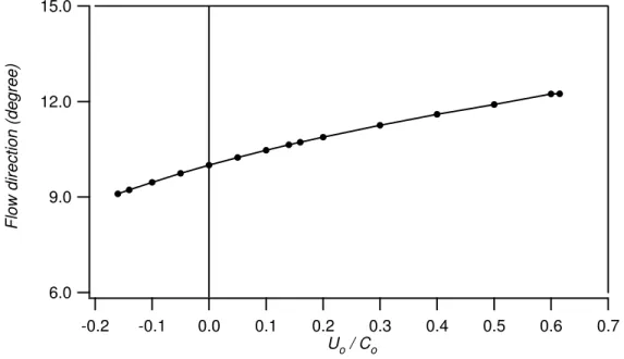
Figs. 6, 7, 8 and 9, respectively shows the variation of the surface disturbance heights, lengths, current like parameters and variation of the direction of the combined wave-current field for the above given conditions.

From Figs. 6 and 7, it is observed that wave with a following current will reduce the resulted wave height and elongate its length and, exactly the opposite incidents take place when current is in the opposite direction of wave. It is also found that the monochromatic wave that we have used in our computation, becomes O(10-3m) (w.r.t. incident wave) when normalized current parameter reaches the value Uo/Co = 0.615 for the case of a wave with a

following current. This is because when wave and current are in the same direction the wave height reduces with current and disappears when the current is strong enough to eliminate the wave amplitude from the combined wave-current field. For the case when wave and current are in opposite directions the maximum wave height is reached at Uo/Co

= -0.16. Maximum wave height is reached due to wave blocking. At this point wave steepness exceeds the allowable breaking value and the numerical model is stopped. The reason is when the wave propagates against an opposite current the wave height increases with current and at some point the wave propagation cannot be persisted (see Zaman and Baddour (2006)). These limits are shown in Fig. 6 by a vertical dotted line.

Fig. 8 shows that the current-like parameter increases when the wave moves with a following current and decreases when they are in opposite directions. In contrast, Fig. 9 shows that the change in the direction of the combined field is much more significant in the case of an opposing current. Figs. 6 to 9 respectively, shows the disturbance height, length, variation of current-like parameters and directions in the combined wave-current field for different current conditions. As expected the surface disturbance height increases with an opposite current and reduces on a following current (Fig. 6) and a reverse behavior is observed for the surface undulation length (Fig. 7). An increase of the current-like parameter is observed for the case of a following current due to wave-induced drift and a reverse behavior is observed for the opposite case (Fig. 8). The variation of the combined wave-current field direction commonly depends on the pre-interaction relative direction of the current-free wave and current fields and magnitude of the current velocity (Fig. 9). 5. Conclusion

Interaction of a current-free long-crested wave and a free current in a 3D wave-current field for irrotational flow conditions has been formulated in terms of conservation of mass, momentum and energy flux and a dispersion relation. Figs. 3a to 5b show the characteristic properties of the particle trajectory with- and without current along an arbitrary direction in the xz plane.

Eqs. (34) to (39) produce the governing conservation equations when Eqs. (27), (29) and (33) are used to formulate the unknown quantities for the cases of wave, current and wave-current conditions. The obtained equations are used for the numerical computation of the combined field parameters. Maple software environment is used for the iterative solution of the nonlinear system of conservation equations and free-surface dispersion relation. In the computations Eqs. (37) to (39) are used to find the direction of the combined wave-current field while Eqs. (34) to (36) together with Eq. (48) are utilized for the computation

(17)

parameter U, and the variation of the direction of the combined wave-current field. An example on the application of the present model has been provided.

References

Baddour, R.E. and Song, S.W. 1990a. On the interaction between waves and currents. Ocean Engineering, 17 (1/2), 1-21.

Baddour, R.E and Song, S.W., 1990b. Interaction of higher-order water waves with uniform currents. Ocean Engineering, 17 (6), 551-568.

Dean, R.G. and Dalrymple, R.A., 1992. Water wave mechanics for engineers and scientists. Prentice-Hall Inc, Englewood Cliffs, NJ, 66-69.

Hedges, T.S. and Lee B.W., 1991. The equivalent uniform in wave-current computations. Coastal Engineering, 16, 301-311.

Kemp, P. H. and Simons R. R. 1982. The interaction between waves and a turbulent current: waves propagating with the current. Journal of Fluid Mechanics, 116, 227-250. Kemp, P. H. and Simons R. R. 1983. The interaction of waves and a turbulent current: waves propagating against the current. Journal of Fluid Mechanics, 130, 73-89.

Longuet-Higgins, M.S. and Stewart, R.W., 1960. Changes in the form of short gravity waves on long waves and tidal currents. Journal of Fluid Mechanics, 8, 565-583.

Longuet-Higgins, M.S. and Stewart, R.W., 1961. The changes in amplitude of short gravity waves on steady non-uniform currents. Journal of Fluid Mechanics, 10, 529-549. Maple-V, Language reference manual, Waterloo Maple Publishing, Springer-Verlag, Heidelberg, NY, 1991.

Whitham, G.B., 1962. Mass, momentum and energy flux in water waves. Journal of Fluid Mechanics, 12, 135-147.

Zaman, M.H., Togashi, H. and Baddour, E., 2008. Deformation of monochromatic water waves propagating over a submerged obstacle in the presence of uniform current. Ocean Engineering, 35 (8-9), 823-833.

Zaman, M.H. and Togashi, H., 1996. Experimental study on interaction among waves, currents and bottom topography. Proceedings Civil Engineering in the Ocean, JSCE, 12, 49-54.

Zaman, M.H. and Baddour, R.E., 2005. Combined loading of a wave and surface current on a fixed vertical slender cylinder. In: 24th International Conference on offshore Mechanics and Arctic Engneering, OMAE-2005, ASME, Halkidiki, Greece, 8pp., on CD-ROM.

Zaman, M. H. and Baddour, R. E. (2006): Wave-current loading on a vertical slender cylinder by two different numerical models, 25th Int. Conf. on offshore Mech. and Arctic

(18)

Eng. (OMAE-2006), American Society of Mechanical Engineers (ASME), Hamburg, Germany, on CD-ROM.

(19)

Fig.1 Wave-free current, current-free wave and wave-current fields relative directions

Fig. 2 Axes orientation in 3D for particle trajectory computation

 x y N S w N Wave field Current field O Wave-current field c N ir w c j r x y x’ xo,,yo,,zo) z, z’ y’ P U

(20)

Fig. 3a Particle trajectory at z’/d=0 Fig. 3b Particle trajectory at z’/d=-0.5 [do = 10m, T = 4s, and Uo/Co =0] [do = 10m, T = 4s, and Uo/Co =0]

Fig. 4a Particle trajectory at z’/d=0 Fig. 4b Particle trajectory at z’/d=-0.5

[do = 10m, T = 4s, and Uo/Co = 0.005] [do = 10m, T = 4s, and Uo/Co = 0.005] -0.010 -0.005 0.000 0.005 0.010 z ' / d -0.010 -0.005 0.000 0.005 0.010 x' / d Wave -0.525 -0.500 -0.475 z ' / d -0.010 -0.005 0.000 0.005 0.010 x' / d Wave -0.025 0.000 0.025 z ' / d -0.050 -0.025 0.000 0.025 0.050 x' / d Wave Current -0.525 -0.500 -0.475 z ' / d -0.050 -0.025 0.000 0.025 0.050 x' / d Wave Current

(21)

Fig. 5a Particle trajectory at z’/d=0 Fig. 5b Particle trajectory at z’/d=-0.5 [do = 10m, T = 4s, and Uo/Co = -0.005] [do = 10m, T = 4s, and Uo/Co = -0.005]

Fig. 6 Variation of wave heights with varying current [do = 5.0m, T = 1.7896s, do/Lo = 1.0, Ho/Lo = 0.05 and Uo/Co varying over the range of –0.2 to 0.6]

-0.025 0.000 0.025 z ' / d -0.050 -0.025 0.000 0.025 0.050 x' / d Wave Current -0.525 -0.500 -0.475 z ' / d -0.050 -0.025 0.000 0.025 0.050 x' / d Wave Current 2.0 1.5 1.0 0.5 0.0 H / H o 0.7 0.6 0.5 0.4 0.3 0.2 0.1 0.0 -0.1 -0.2 U_o / C_o

Maximum wave height is reached at Uo/Co = -0.16

Wave height is of O(10-3 m) at Uo/Co = 0.615

(22)

Fig. 7 Variation of wavelengths with varying current [do = 5.0m, T = 1.7896s, do/Lo = 1.0, Ho/Lo = 0.05 and Uo/Co varying over the range of –0.2 to 0.615]

Fig. 8 Variation of current-like parameter [do = 5.0m, T = 1.7896s, do/Lo = 1.0, Ho/Lo =

0.05 and Uo/Co varying over the range of –0.2 to 0.615]

2.5 2.0 1.5 1.0 0.5 0.0 L / Lo 0.7 0.6 0.5 0.4 0.3 0.2 0.1 0.0 -0.1 -0.2 U_o / C_o -100.0 -50.0 0.0 50.0 (U-U o )/C o X 10 4 0.7 0.6 0.5 0.4 0.3 0.2 0.1 0.0 -0.1 -0.2 U_o / C_o

(23)

Fig. 9 Variation of the combined wave-current field direction with varying current [do =

5.0m, T = 1.7896s, do/Lo = 1.0, Ho/Lo = 0.05 and Uo/Co varying over the range of –0.2 to

0.615] 15.0 12.0 9.0 6.0 F lo w dir e ction ( d e g ree) 0.7 0.6 0.5 0.4 0.3 0.2 0.1 0.0 -0.1 -0.2 U_o / C_o