Publisher’s version / Version de l'éditeur:
Proceedings of the 2012 Fall Technical Conference of the ASME Internal
Combustion Engine Division (ICEF2012), pp. 657-666, 2012-09-26
READ THESE TERMS AND CONDITIONS CAREFULLY BEFORE USING THIS WEBSITE. https://nrc-publications.canada.ca/eng/copyright
Vous avez des questions? Nous pouvons vous aider. Pour communiquer directement avec un auteur, consultez la première page de la revue dans laquelle son article a été publié afin de trouver ses coordonnées. Si vous n’arrivez pas à les repérer, communiquez avec nous à PublicationsArchive-ArchivesPublications@nrc-cnrc.gc.ca.
Questions? Contact the NRC Publications Archive team at
PublicationsArchive-ArchivesPublications@nrc-cnrc.gc.ca. If you wish to email the authors directly, please see the first page of the publication for their contact information.
NRC Publications Archive
Archives des publications du CNRC
This publication could be one of several versions: author’s original, accepted manuscript or the publisher’s version. / La version de cette publication peut être l’une des suivantes : la version prépublication de l’auteur, la version acceptée du manuscrit ou la version de l’éditeur.
For the publisher’s version, please access the DOI link below./ Pour consulter la version de l’éditeur, utilisez le lien DOI ci-dessous.
https://doi.org/10.1115/ICEF2012-92191
Access and use of this website and the material on it are subject to the Terms and Conditions set forth at
Real-time monitoring of combustion instability in a homogeneous
charge compression ignition (HCCI) engine using cycle-by-cycle
exhaust temperature measurements
Gardiner, David P.; Neill, W. Stuart; Chippior, Wallace L.
https://publications-cnrc.canada.ca/fra/droits
L’accès à ce site Web et l’utilisation de son contenu sont assujettis aux conditions présentées dans le site LISEZ CES CONDITIONS ATTENTIVEMENT AVANT D’UTILISER CE SITE WEB.
NRC Publications Record / Notice d'Archives des publications de CNRC:
https://nrc-publications.canada.ca/eng/view/object/?id=5d9141ee-b2d3-4fa3-95b4-ebd8264614b5 https://publications-cnrc.canada.ca/fra/voir/objet/?id=5d9141ee-b2d3-4fa3-95b4-ebd8264614b5
Proceedings of the ASME 2012 Internal Combustion Engine Division Fall Technical Conference ICEF2012 September 23-26, 2012, Vancouver, BC, Canada
ICEF2012-92191
REAL-TIME MONITORING OF COMBUSTION INSTABILITY IN A HOMOGENEOUS
CHARGE COMPRESSION IGNITION (HCCI) ENGINE USING CYCLE-BY-CYCLE
EXHAUST TEMPERATURE MEASUREMENTS
David P. GardinerNexum Research Corporation Mallorytown, Ontario, Canada
W. Stuart Neill National Research Council
Ottawa, Ontario, Canada
Wallace L. Chippior National Research Council
Ottawa, Ontario, Canada
ABSTRACT
This paper describes an experimental study concerning the feasibility of monitoring the combustion instability levels of an HCCI engine based upon cycle-by-cycle exhaust temperature measurements. The test engine was a single cylinder, four-stroke, variable compression ratio Cooperative Fuel Research (CFR) engine coupled to an eddy current dynamometer. A rugged exhaust temperature sensor equipped with special signal processing circuitry was installed near the engine exhaust port. Reference measurements were provided by a laboratory grade, water-cooled cylinder pressure transducer. The cylinder pressure measurements were used to calculate the Coefficient of Variation of Indicated Mean Effective Pressure (COV of IMEP) for each operating condition tested.
Experiments with the HCCI engine confirmed that cycle-by-cycle variations in exhaust temperature were present, and were of sufficient magnitude to be captured for processing as high fidelity signal waveforms. There was a good correlation between the variability of the exhaust temperature signal and the COV of IMEP throughout the operating range that was evaluated. The correlation was particularly strong at the low levels of COV of IMEP (2-3%), where production engines would typically operate.
A real-time combustion instability signal was obtained from cycle-by-cycle exhaust temperature measurements, and used to provide feedback to the fuel injection control system. Closed loop operation of the HCCI engine was achieved in which the engine was operated as lean as possible while maintaining the COV level at or near 2.5%.
INTRODUCTION
Advanced combustion strategies such as homogeneous charge compression ignition (HCCI) offer the potential for diesel-like fuel conversion efficiency and very low levels of the two
problematic emissions associated with conventional diesel combustion, namely soot and NOx. At high loads, the operating range where HCCI can be used is limited by knock. At low loads operation is limited by excessive cycle-to-cycle variations in Indicated Mean Effective Pressure (IMEP) due to combustion instability [1,2]. Effective knock sensors are currently available, and have been evaluated for feedback control of HCCI engines [3]. A practical sensor providing a combustion instability feedback signal would facilitate operation at or near the lean stability limit at light loads, thus providing a valuable enabling technology for these engines.
In laboratory research and development applications, cyclic variability is quantified by the Coefficient of Variation of Indicated Mean Effective pressure, based upon cylinder pressure measurements. Cylinder pressure sensors have been developed that are intended for continuous use in production engines, but have yet to see widespread use. Other approaches to determining cyclic variability include those based on measurements or crankshaft velocity, and ion current measurements from spark plugs. Ion current measurements and the use of microphones and knock sensors have been evaluated with HCCI engines [3,4].
In the present study, cyclic variability levels were determined based upon the sensing of cycle-by-cycle fluctuations in the exhaust temperature measured by a durable sheathed thermocouple located near the exhaust port. The thermocouple used was similar to those commonly used in large stationary engine and gas turbine applications. Proprietary circuitry and signal processing were used to extract high frequency information from the thermocouple.
Each cylinder of a multi-cylinder engine may be monitored individually as long as the exhaust manifold design and the thermocouple location ensure that the thermocouple is not exposed to substantial exhaust flow from the adjacent cylinders.
Isolation of the exhaust flow has proven to be relatively easy to achieve in practice, and a wide variety of multi-cylinder engines (up to 12 cylinders) have been monitored successfully. This technology offers many of the benefits of cylinder pressure based combustion monitoring systems, but avoids the need for cylinder head modifications to provide access to the combustion chamber for the cylinder pressure sensors.
Previous investigations with conventional spark ignition engines have demonstrated that a correlation exists between the cycle-by-cycle variability of the exhaust temperature fluctuations of a cylinder and the COV of IMEP determined from cylinder pressure measurements of the corresponding cycles [5,6]. This relationship has also been noted by other researchers using fragile, fine wire thermocouples [7]. For conventional spark ignition engines, increasing cyclic variability of combustion phasing is the underlying cause of increases in the COV of IMEP [8]. The correlation between cycle-by-cycle exhaust temperatures and the COV of IMEP exists because the changes in cycle-by-cycle exhaust temperatures reflect changes in the combustion phasing of the cycles, with slower burning cycles producing later combustion phasing and correspondingly high gas temperatures at the time of exhaust valve opening [5,7].
It has been shown that HCCI engines encounter increased COV of IMEP levels at low loads due to a different mechanism. In this case, cycle-to-cycle variations in the total heat released are the main contributor to cyclic variability in IMEP [1,2]. At the outset of the current study, it was unclear whether or not this mechanism would lead to cycle-by-cycle variations in exhaust temperature that would be sufficient to enable changes in the COV of IMEP to be detected.
This paper describes an experimental study in which the relationship between the COV of IMEP of an HCCI engine and the variability of the corresponding cycle-by-cycle exhaust temperature measurements was determined. The operating conditions that were evaluated included variations in air/fuel ratio, different levels of exhaust gas recirculation, and different compression ratios. The paper also presents the results of work intended to provide a real-time COV signal from the exhaust temperature measurements, and implement the signal in a closed loop control system. The latter results are of relevance not only to HCCI engines, but also to other engine types such as lean burn natural gas engines.
BACKGROUND
The method of monitoring cycle-by-cycle exhaust temperatures used in the study is based upon the work originally carried out by Shepard and Warshawsky over fifty-five years ago. In studies conducted by the National Advisory Committee for Aeronautics (NACA, the forerunner of NASA), they developed a means of obtaining information about high frequency temperature fluctuations in gas flows while using relatively large, exposed junction thermocouples [9]. They showed that the actual dynamic gas temperature could be reconstructed based upon the indicated temperature signal, the time constant of the
thermocouple, and the rate of change of the thermocouple signal. The adaptation of the Shepard and Warahawsky technique for monitoring cycle-by-cycle combustion variations was introduced in an earlier paper [10], and is described briefly in the following portion of the present paper.
A thermocouple produces a millivolt signal that reflects the temperature of the thermocouple wire in the vicinity of the thermocouple junction. The instantaneous gas temperature (Tg)
can be obtained from the wire temperature signal (Tw) using the
following equation: = + w g w dT T T dt t (1)
where t is the time constant of the thermocouple for convective heat transfer from the gas. Shepard and Warshawsky determined the time constant by calibrating the response of the thermocouple to step changes in the temperature of gas flows.
The value that is added to the wire temperature signal to obtain the instantaneous gas temperature tdTw
dt may be
referred to as the dynamic temperature correction. If the thermocouple is large enough, Tw will change very little during
the period typical of several engine cycles. Thus, the cycle-by-cycle temperature fluctuation of the engine exhaust will be described by the dynamic temperature correction alone.
Furthermore, the value of the time constant, t, can be considered as a scaling factor applied to the derivative of the thermocouple signal to produce the dynamic temperature correction. Thus, the shape of the cycle-by-cycle temperature fluctuations (i.e., an un-scaled version of the exhaust temperature waveform) is indicated solely by the derivative of the thermocouple signal. This makes it unnecessary to completely reconstruct the instantaneous exhaust gas temperature in order to obtain the relative cycle-by-cycle variability of the exhaust temperature. The information needed to detect changes in cyclic combustion instability can be obtained directly from the derivative signal.
Practical engine thermocouples use sheathed probe configurations (where the thermocouple wire and junction are protected by a protective jacket), as exposed junction thermocouple would corrode too rapidly to provide adequate durability. The sheathed configuration results in slower transient response than an exposed junction, making it difficult to obtain a derivative signal with a tolerable signal-to-noise ratio.
A modest, but valuable improvement in transient response can be achieved by reducing the diameter of the thermocouple tip, while retaining a relatively large diameter for most of the thermocouple length that is exposed to the exhaust flow. If the entire thermocouple had a smaller diameter, the greater length-to-diameter ratio would make the thermocouple vulnerable to fatigue failure due to vibrations caused by the gas flow. The use reduced tip thermocouples as a means of improving response/durability trade-offs is well established in gas turbine applications.
Nevertheless, the transient response of such thermocouples is far too slow to reveal cycle-by-cycle exhaust temperature fluctuations through conventional signal analysis. The combustion instability monitoring system discussed in the remainder of the paper employed proprietary signal processing techniques to obtain a useable exhaust temperature waveform signal from the reduced tip, sheathed thermocouples.
EXPERIMENTAL SETUP AND PROCEDURE
Research Engine
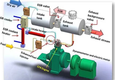
Figure 1 is a schematic diagram of the HCCI combustion research facility used in this study. The Cooperative Fuel Research (CFR) engine, a single-cylinder, four-stroke, variable compression ratio engine, was coupled to an eddy current dynamometer. The CFR engine is widely used for determination of cetane and octane numbers of diesel and gasoline fuels, respectively. The octane number version of the CFR engine was used in this study, as the cetane version employs a pre-chamber configuration that is not suitable for HCCI combustion. Table 1 provides the basic engine specifications.
The engine setup was modified from the standard configuration by the addition of an air-assisted port fuel injection system and hardware to control critical engine parameters such as intake temperature, air/fuel ratio, intake and exhaust pressures, and Exhaust Gas Recirculation (EGR). A port fuel injector was used to atomize the fuels upstream of the intake port. Compressed air, taken from the intake air after the mass flow meter, was used as blast air to improve the atomization process. For this study, the fuel and air-blast pressures were maintained at 500 kPa and 200 kPa, respectively. The air blast was delivered to the fuel atomizer using a gaseous fuel injector at the same time and with the same duration as the liquid fuel injection. Experimental data suggests that this fuel injector produces droplets with approximately 15 micrometer Sauter mean diameter under the conditions used in this study.
Figure 1: Schematic of HCCI Combustion Research Facility
Table 1: CFR Engine Specifications
Engine Waukesha Cooperative Fuel Research
(CFR)
Combustion
chamber Flat top piston, pancake
Compression ratio Variable, 6:1 to 16:1 ( In this study changed from 9:1 to 13.5:1)
Bore × Stroke 82.55 × 114.3 mm Displacement 611.7 cc
Intake valve open 10°CA, aTDC Intake valve close 34°CA, aBDC Exhaust valve open 40°CA, bBDC Exhaust valve close 5°CA, aTDC
Fuel System Air-blast assist port fuel injection A heated section was added downstream of the fuel injector to partially-vaporize the lower boiling point fuel components. Figure 2 shows the details of the fuel injector/vaporizer.
Figure 2: Schematic of the Enhanced Port Fuel Injector/Vaporizer
The intake mixture temperature (Tmix) was measured in the
intake port downstream of the fuel vaporizer. The intake air was provided from a pressurized dry air source. The intake air flow was measured by a mass flow meter before entering the intake surge tank, where the air was mixed with recycled exhaust gases (when desired). The EGR and air mixture then passed through a lengthy intake system, which provided additional time to achieve a homogeneous mixture and avoid large fluctuations in the EGR level. One of the elements of the intake system was a heat exchanger to cool the EGR and air. The heat exchanger coolant was heated to just below the intake air temperature to avoid water vapor condensation. The heat exchanger was sized appropriately to compensate for the small temperature difference. An intake heater was used to maintain the intake air and EGR at the desired temperature.
The engine exhaust was routed through an exhaust surge tank equipped with a safety rupture disk. A back pressure valve was used to maintain the exhaust pressure slightly above the intake pressure to provide the pressure drop needed to recycle exhaust gases to the intake stream. An engine data acquisition
and control system (Sakor Technologies Inc., DynoLab™) was used to acquire temperatures, pressures, and flow rates. A water-cooled pressure transducer (Kistler Corp., model 6041A) flush-mounted in the cylinder head was used to measure combustion pressure. The cylinder pressure data was acquired for 300 consecutive engine cycles with 0.2°CA resolution using a real-time combustion analysis system (AVL LIST GmbH, IndiModule). All experiments were performed under steady state conditions.
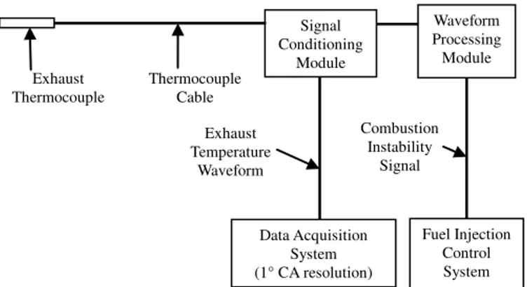
Combustion Instability Monitoring System
The combustion instability monitoring system is depicted in Figure 3. The exhaust temperature probe was a grounded junction, hastalloy-sheathed chromel-alumel thermocouple with a shaft diameter of 4.8 mm (3/16”). The tip was tapered to a minimum diameter of 2.4 mm (3/32”). Unlike the design used in some earlier studies [5,6], there were no electronic components near the probe. The un-amplified thermocouple signal was delivered to the signal conditioning module (located in the test cell control room) via a proprietary low-noise cable design approximately 10 meters in length. This feature (a passive sensor combined with a long cable) was originally developed for use with stationary natural gas engines in applications where powered sensor would be undesirable due to the potential presence of flammable gases.
The signal conditioning module contained circuitry that extracted the cycle-by-cycle temperature waveform from the raw thermocouple signal. As discussed earlier, no attempt was made to determine the actual temperature of this waveform. For this study, the signal was low-pass filtered with a cutoff frequency of 40 Hz and time-based sampling of the signal was done at 1 kHz.
This signal was recorded, along with cylinder pressure, by the crank-angle-based data acquisition system. For the cyclic variability comparisons presented later in the paper, 300 consecutive cycles were recorded simultaneously from the cylinder pressure and temperature waveform signals. The COV of IMEP and COV of the temperature waveform were determined through post processing of the recorded signals
Figure 3: Combustion Instability Monitoring System
The temperature waveform signal was also delivered to the signal processing module. The circuitry in this module produced an analog voltage proportional to the COV of the temperature waveform. During some tests, this real-time COV signal was used as a feedback signal by the fuel injection control system in order to achieve closed loop control of the air/fuel ratio at a target COV level.
Test Conditions
All of the tests were carried out at a speed of 900 rpm. This relatively low engine speed was a typical test condition for this particular HCCI engine rather than a limitation of the exhaust temperature monitoring system, as the system has been demonstrated at speeds as high as 5000 rpm with conventional spark ignition engines.
Five different baseline test conditions were used. In each case, a range of values for the COV of IMEP were produced. This was accomplished by varying the air/fuel ratio in four of these cases. In one case, a constant air/fuel ratio was used and the COV of IMEP was changed by varying the compression ratio. Either 60% EGR or no EGR was used. The tests were run at a fixed value of Inlet Manifold Absolute Pressure, and the fuel flow or the compression ratio was varied. Consequently, the IMEP varied from about 5 bar (near the knock limit) down to a <2.5 bar near the stability limit.
The fuel for four of the test conditions was a 50/50 blend of isooctane and n-heptane. Diesel fuel (commercial, winter grade low sulfur diesel) was used for one of the test conditions, which enabled operation at a relatively low compression ratio of 9:1.
The experimental matrix was intended primarily to produce a range of COV of IMEP values ranging from about 1.5-2% (very stable combustion) to about 5% (a level that would be considered excessively high for most modern engines). The objective was to achieve this range of COV values using different combinations of compression ratio, EGR rate, air/fuel ratio and fuel type. The combinations of these variables that were used were selected because prior experience from other experimental studies had indicated that these combinations could produce the desired range of COV of IMEP values. RESULTS AND DISCUSSION
Exhaust Temperature Waveforms and COV Calculation
Examples of 10 consecutive cycles of the cycle-by-cycle exhaust temperature waveforms at two different levels of cyclic variability are shown in Figures 4 and 5. The scaling shows the rate of change of the indicated thermocouple temperature which, as discussed earlier, provides an indication of the relative magnitude of cycle-to-cycle fluctuations in the exhaust temperature. It can be seen that the signal processing circuitry produced very high fidelity signal waveforms, despite the use of a slow-responding sheathed thermocouple.
In Figure 4, the waveform appearance is similar to that reported by other researchers using fine wire thermocouples and
Signal Conditioning Module Waveform Processing Module Exhaust Thermocouple Thermocouple Cable Data Acquisition System (1° CA resolution) Fuel Injection Control System Combustion Instability Signal Exhaust Temperature Waveform
resistance thermometers [11-13]. The exhaust temperature rises abruptly during the period when the exhaust valve is open (due to blowdown and displacement flow of hot exhaust past the probe), then cools at a slower rate while the exhaust valve is closed. -8 -6 -4 -2 0 2 4 6 8 10 0 1 2 3 4 5 6 7 8 9 10 Cycle 1.7% COV of IMEP S ignal D er iv at iv e (° C /s )
Figure 4: Example of Exhaust Temperature Waveform from Operation at Low COV of IMEP
-8 -6 -4 -2 0 2 4 6 8 10 0 1 2 3 4 5 6 7 8 9 10 Cycle 4.6% COV of IMEP S ignal D er iv at iv e (° C /s )
Figure 5: Example of Exhaust Temperature Waveform from Operation at High COV of IMEP
-6 -4 -2 0 2 4 6 8 10 0 90 180 270 360 450 540 630 720
Crank Angle (deg) 1.7% COV of IM EP S ig n al D er iv ativ e ( °C /s )
Figure 6: 50 Consecutive Cycles of Exhaust Temperature Waveform from Operation at Low COV of
IMEP -6 -4 -2 0 2 4 6 8 10 0 90 180 270 360 450 540 630 720
Crank Angle (deg)
S ig n al D er iv ativ e ( °C /s ) 4.6% COV of IM EP
Figure 7: 50 Consecutive Cycles of Exhaust Temperature Waveform from Operation at High COV
of IMEP
There are noticeable differences between the waveforms in Figures 4 and 5 that are a reflection of the greater combustion instability when the COV of IMEP was higher. There are greater cycle-to-cycle variations in the waveform as the COV level approaches 5%, and some cycles produce temperature rises that are markedly lower than the adjacent cycles. The relationship between the cyclic variation of the temperature waveform and the COV of IMEP is also evident in Figures 6 and 7, where 50 consecutive cycles have been over-plotted in each case.
The cyclic dispersion of the exhaust temperature waveform may be quantified using a variety of algorithms [14]. In each case, a value must be determined for each cycle so that the cyclic dispersion of groups of cycles may be calculated. This is complicated somewhat by the existence of prior-cycle effects, as the minimum temperature of the previous cycle (just before exhaust valve opening) will affect the peak value of the current cycle.
The parameter used in the current study was the magnitude of the signal rise for each cycle. That is, the difference between the minimum value at the beginning of the cycle and the peak value reached during the cycle. The cyclic variability of groups of cycles was quantified as the COV of these cycle-by-cycle signal rise values, calculated in the same manner as the COV of IMEP (standard deviation/mean x 100). Like the COV of IMEP, normalizing the standard deviation of the group of cycles by the mean of the group makes it unnecessary to obtain signal measurements with high accuracy.
Relationship Between COV of ETW and COV of IMEP Figure 8 shows the relationship between the COV of the exhaust temperature waveform and the COV of IMEP for the 5 test conditions. In Figures 8A and 8B, tests were run without EGR
in which the COV of IMEP was increased by making the air/fuel ratio leaner. These tests were run at compression ratios of 12:1 and 9:1 using 50/50 iso-octane/n-heptane and diesel fuel respectively. The air/fuel ratios are expressed as the excess air ratio, or lambda. The lambda values (over 4 in some cases) appear to be extremely lean relative to normal expectations for premixed charge engines, but are typical for HCCI engines while operating without EGR.
In both cases there was a strong, nearly linear relationship between the COV of the exhaust temperature waveform and the COV of IMEP. In particular, it was possible to detect changes in the COV of IMEP in the region of 2-3% COV. This is relevant because these would be desirable COV levels for the operation of automotive engines.
A: 12:1 CR, 0% EGR, Variable Lambda
4 6 8 10 12 14 16 1 2 3 4 5 COV of IMEP (%) C O V o f ET W (% ) 3 4 5 6 Lam bda COV of ETW Lambda
B: 9:1 CR, 0% EGR, Variable Lambda, Diesel Fuel
4 9 14 19 24 1 2 3 4 5 6 7 COV of IMEP (%) C O V o f ET W (% ) 2 3 4 5 Lam bda COV of ETW Lambda
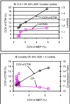
C: 13.5:1 CR, 60% EGR, Variable Lambda
4 6 8 10 12 14 16 18 1 2 3 4 5 6 COV of IMEP (%) C O V o f ET W (% ) 1 2 3 Lam bda COV of ETW Lambda
D: 10.5:1 CR, 60% EGR, Variable Lambda
4 6 8 10 12 14 16 18 20 2 3 4 5 6 COV of IMEP (%) C O V o f ET W (% ) 1 1.1 1.2 1.3 1.4 1.5 Lam bda COV of ETW Lambda
E: Variable CR, 60% EGR, 1.2 Lambda
4 6 8 10 12 14 16 1 2 3 4 COV of IMEP (%) C O V o f ET W (% ) 10 11 12 13 14 15 16 C om pr es s ion R at io CR COV of ETW
Figure 8: COV of Exhaust Temperature Waveform (ETW) versus COV of IMEP at Different Engine
Operating Conditions
Similar results can be seen in Figures 8C and 8D, where 60% EGR and moderately lean air/fuel ratios (lambda < 2) were used at compression ratios of 13.5:1 and 10.5:1 respectively. With the lower compression ratio, the COV of IMEP was very sensitive to air/fuel ratio once the mixture was very sensitive to air/fuel ratio, and rose abruptly from about 3% to 5% when the mixture became about 3% leaner. The ability to detect changes in the COV of IMEP in the region of 2-3% was evident in both cases.
For the results shown in Figure 8E, the air/fuel ratio was held constant while the compression ratio was varied. The COV of IMEP remained at extremely low levels (<1.5% COV) as the compression ratio was changed until the compression ratio was less than 11:1. At this point, further decreases in the compression ratio led to abrupt increases in the COV of IMEP. Only one operating point fell within the area of interest (2-3% COV), but the trends shown on the graph suggest that it would be possible for the COV of ETW to be used to detect changes in the COV of IMEP in this region under variable compression ratio operation.
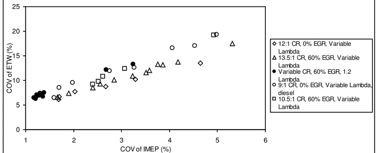
0 5 10 15 20 25 1 2 3 4 5 6 COV of IMEP (%) C O V o f ET W (% ) 12:1 CR, 0% EGR, Variable Lambda 13.5:1 CR, 60% EGR, Variable Lambda Variable CR, 60% EGR, 1.2 Lambda
9:1 CR, 0% EGR, Variable Lambda, diesel
10.5:1 CR, 60% EGR, Variable Lambda
Figure 9: COV of Exhaust Temperature Waveform (ETW) versus COV of IMEP for all Engine Operating Condition
Figure 9 shows the relationship between the COV of ETW and the COV of IMEP for all of the operating conditions shown earlier in Figure 8. It can be seen that the relationship varied somewhat between the different conditions. This suggests that a control strategy based upon cycle-by-cycle temperature monitoring would require some sort of mapping of the control setpoint (as a function of operating parameters) in order to maintain the COV of IMEP at a constant level.
Real-Time COV Feedback Signal for Closed Loop Control
It should be emphasized that the objective of the technology was not to measure the COV of IMEP over a wide range, but instead was to detect if the COV level was above or below a predetermined threshold level, appropriate for acceptable, stable operation of the engine. This would be analogous to the use of a conventional Exhaust Gas Oxygen (EGO) sensor, where a strong change in the signal is produced in the vicinity of the desired operating point. To this end, the development of real-time processing capabilities for the exhaust temperature waveform signal was focused on producing a signal that would be effective for providing effective control system feedback for maintaining a COV of IMEP level between about 2-3%.
A proprietary signal processing circuit was developed that produced a 0-10 Volt analog signal in response to variations in the cycle-by-cycle variability of the ETW signal. Initial test were conducted in which this signal was used to provide feedback to the closed loop control system used to vary the pulse duration of the fuel injector. The response of the signal to changes in the COV of IMEP under the operating conditions used for the tests (12:1 compression ratio, 0% EGR) is shown in Figure 10. The signal was calibrated to provide 2.5 volts when the COV of IMEP was 2.5%. The data shown is the mean value
of the analog signal during the period when corresponding 300 cylinder pressure cycles were recorded. It can be seen that the signal response was not linear, but provided a strong increase in voltage once the COV of IMEP exceeded about 2.5%
2 2.5 3 3.5 4 4.5 1 2 3 4 5 COV of IMEP (%) ET W C O V Si g n a l (V)
Figure 10: Real-Time COV Signal versus COV of IMEP (12:1 CR, 0% EGR)
In these initial closed loop control experiments, online signal averaging techniques were used such that the feedback signal was essentially a moving average of about 200 cycles (25 seconds at the 900 rpm test condition). The time constant of control system was similar. COV of IMEP values from the cylinder pressure system are not shown in the following figures because this system was only suitable for steady-state operating conditions.
The perturbation in operating conditions used for the control experiments was accomplished through a step change in inlet pressure. In Figures 11 and 12, an increase in inlet pressure (10 kPa and 20 kPa, respectively) was used to make the mixture
leaner. The leaner mixture caused an increase in combustion instability, leading to an increase in the COV signal above the control system setpoint of 2.5 Volts. This caused the fuel control system to increase the fuel injector pulsewidth, resulting in reduction in the excess air ratio (lambda) until the target COV level of 2.5% was restored.
115 125 135 145 155 165 0 25 50 75 100 125 150 Time (s) Inl et P re ss ure (kP a) P Inlet 1.5 2 2.5 3 3.5 4 0 25 50 75 100 125 150 Time (s) CO V S igna l (V ) COV 2.5 2.75 3 3.25 3.5 3.75 4 0 25 50 75 100 125 150 Time(s) Inj ec tor P ul se w idt h (m s) Injector 3 3.5 4 4.5 5 5.5 6 0 25 50 75 100 125 150 Time (s) L am b d a Lambda
Figure 11: Closed Loop Response to 10 kPa Increase in Inlet Pressure 115 125 135 145 155 165 0 25 50 75 100 125 150 Time (s) Inl et P re ss ure (kP a) P Inlet 1.5 2 2.5 3 3.5 4 0 25 50 75 100 125 150 Time (s) CO V S igna l (V ) COV 2.5 2.75 3 3.25 3.5 3.75 4 0 25 50 75 100 125 150 Time (s) Inj ec tor P ul se w idt h (m s) Injector 3 3.5 4 4.5 5 5.5 6 0 25 50 75 100 125 150 Time (s) L am b d a Lambda
Figure 12: Closed Loop Response to 20 kPa Increase in Inlet Pressure
115 125 135 145 155 165 0 50 100 150 200 250 Time (s) Inl et P re ss ure (kP a) P Inlet 1.5 2 2.5 3 3.5 4 0 50 100 150 200 250 Time (s) CO V S igna l (V ) COV 2.5 2.75 3 3.25 3.5 3.75 4 0 50 100 150 200 250 Time (s) Inj ec tor P ul se w idt h (m s) Injector 3 3.5 4 4.5 5 5.5 6 0 50 100 150 200 250 Time (s) L am b d a Lambda
Figure 13: Closed Loop Response to 40 kPa Decrease in Inlet Pressure
Note that in both examples, the control system did not simply restore the original lambda value, as would be the case if a wide range oxygen sensor was used for feedback. The final
lambda value after the control loop was stable again was leaner than the original value. This was likely due to the greater IMEP of the second condition, which made it possible to maintain the 2.5% COV level at a leaner air/fuel ratio.
In Figure 13, a decrease in inlet pressure (of 40 kPa) was used to make the mixture less lean. The decrease in the excess air ratio caused a reduction in combustion instability and the COV signal fell below the control system setpoint of 2.5 Volts. This caused the fuel control system to reduce the fuel injector pulsewidth. Consequently, the excess air ratio (lambda) increased until the target COV level of 2.5% was restored. In this case the final lambda value was less than the original value. This is attributed to the lower IMEP in the second condition, which made it necessary to reduce the excess air ratio to achieve the desired COV level.
The examples of control system response shown in the Figures 11-13 would be much too slow for automotive engines. Further work is required to achieve faster transient response. However, the current control loop response would likely be adequate for stationary engine applications involving continuous operation at a constant speed and load. For example, a lean burn natural gas engine could be use closed loop control of the air/fuel ratio to maintain an acceptable COV level in the presence of changes in the composition of well gas or landfill gas.
Future Studies
The present study addressed the overall correlation between the variability of the ETW signal and the COV of IMEP. As such, the study was concerned with relatively large sets of cycles rather than individual cycles. Future studies should examine the correlation between cycle-by-cycle ETW and IMEP values for HCCI combustion. Cycle-by-cycle comparisons with heat release measurements would be expected to reveal more information about the cause and effect relationship between cycle-by-cycle variations in the HCCI combustion process and the variations observed in the cycle-by-cycle exhaust temperature signal.
SUMMARY AND CONCLUSIONS
An experimental study was carried out to evaluate the potential of cycle-by-cycle exhaust temperature measurements to monitor the cyclic combustion instability of a single cylinder HCCI research engine. Special circuitry was used to obtain cycle-by-cycle temperature information from a durable sheathed thermocouple mounted near the exhaust port. These measurements were compared with the Coefficient of Variation of Indicated Mean Effective Pressure (COV of IMEP) calculated from cylinder pressure measurements from a laboratory grade, water-cooled cylinder pressure transducer. A real-time COV signal from the cycle-by-cycle exhaust temperature measurements was evaluated as a feedback signal for closed loop control of the fuel injection system.
1. The HCCI engine and operating conditions used in this study produced cycle-by-cycle variations in exhaust temperature that could be measured by the signal conditioning circuitry as high fidelity cycle-by-cycle signal waveforms, despite the use of a durable but slow-responding sheathed thermocouple as the temperature sensing element. 2. There was a good correlation between the variability of the
cycle-by-cycle exhaust temperature signal and the COV of IMEP throughout the operating range that was evaluated. The correlation was particularly strong at the low levels of COV of IMEP (2-3%), where production engines would typically operate.
3. A real-time combustion instability signal was obtained from the cycle-by-cycle exhaust temperature waveform. This signal was shown to reflect changes in the COV of IMEP, especially when the COV of IMEP changed from less than to greater than 2.5%.
4. The real-time combustion instability signal was used to provide feedback to a fuel injection control system. Closed loop operation of the HCCI engine was achieved in which the engine was operated as lean as possible while maintaining the COV of IMEP level at or near 2.5%.
ACKNOWLEDGMENTS
The authors gratefully acknowledge financial support for this work from Canada’s Program of Energy Research and Development, the PERD AFTER Program, Projects C23.005 and C22.001.
REFERENCES
1. Li, H., Neill, W.S., Chippior, W, and Taylor, J.D., “An Experimental Investigation of HCCI Combustion Stability Using N-Heptane”, ICEF2007-1757, Proceedings of ICEF2007 ASME Internal Combustion Engine Division 2007 Fall Technical Conference, October 14-17, 2007, Charleston, SC, USA.
2. Ghazimirsaied, A, Shahbakhti, M., and Koch, C.R., “Comparison of Crankangle Based Ignition Timing Methods on an HCCI Engine”, ICEF2010-35087, Proceedings of the ASME 2010 Internal Combustion Engine Division Fall Technical Conference, September 12-15, 2010, San Antonio, TX, USA
3. Souder, J.S., Mack, J.H., Hedrick, J.K., and Dibble, R.W., “Microphones and Knock Sensors for Feedback Control of HCCI Engines”, ICEF2004-960, Proceedings of ICEF2004 ASME Internal Combustion Engine Division 2004 Fall Technical Conference, October 24-27, Long Beach, CA, USA.
4. Bogin, G., Mack, J.H., and Dibble, R.W., “Spark Plug Modifications for Improving Ion Sensing Capabilities in a Homogeneous Charge Compression Ignition (HCCI) Engine”, ICES2009-76161, Proceedings of ICEs2009 ASME Internal Combustion Engine Division 2009 Spring Technical Conference, May 3-6, Milwaukee, WI, USA.
5. Gardiner, D.P and Bardon, M.F., “A Cyclic Variability Monitoring System Based Upon Cycle Resolved Exhaust Temperature Sensing”, ICEF2005-1294, Proceedings of ICEF2005 ASME Internal Combustion Engine Division 2005 Fall Technical Conference, September 11-14, 2005, Ottawa, ON Canada.
6. Gardiner, D.P., Allan, W.D., LaViolette, M., and Bardon, M.F., “Cycle-by-Cycle Exhaust Temperature Monitoring for Detection of Misfiring and Combustion Instability in Reciprocating Engines”, ICEF2007-1740, Proceedings of ICEF2007 ASME Internal Combustion Engine Division 2007 Fall Technical Conference, October 14-17, 2007, Charleston, SC, USA.
7. Kar, K., Swain, A., and Raine, R., “Cycle-by-Cycle Variations in Exhaust Temperature Using Thermocouple Compensation Techniques”, SAE Paper #2006-01-1197, Society of Automotive Engineers, Warrendale PA, 2006 8. Nakajima, Y., Sugihara, Y., Takagi, Y., and Muranaka, S.,
“Effects of Exhaust Gas Recirculation on Fuel Consumption”, Proc. Instn. Mech. Engrs., vol. 195, pp 369-376, London, 1981.
9. Shepard, C.E. and Warshawsky, L., “Electrical Techniques for Compensation of Thermal Time Lag of Thermocouples and Resistance Thermometer Elements”, Technical Note 2703, NACA, Washington D.C., May 6, 1952.
10. Gardiner, D.P., “Misfire Detection for Spark Ignition Engines Based Upon Cycle-by-Cycle Exhaust Temperature Sensing”, ICEF2010-35153, Proceedings of the ASME 2010 Internal Combustion Engine Division Fall Technical Conference, September 12-15, 2010, San Antonio, TX, USA
11. Kar, K., Roberst, S., Stone, R., Oldfield, M., and French, B., “Instantaneous Exhaust Temperature Measurements Using Thermocouple Compensation Techniques”, SAE Paper #2004-01-1418, Society of Automotive Engineers, Warrendale PA, 2004.
12. Mollenhaurer, K., “Measurement of Instantaneous Gas Temperatures for Determination of the Exhaust Gas Energy of a Supercharged Diesel Engine”, SAE Paper #670929, Society of Automotive Engineers, Warrendale PA, 1967. 13. Benson, R.S., “Measurement of the Transient Exhaust
Temperature in I.C. Engines”, The Engineer, Feb. 1964, pp 377-383.
14. Gardiner, D.P., “Method and Apparatus for Monitoring Cyclic Variability in Reciprocating Engines”, U.S. Patent No. US 7,461,545 B2, Dec 9, 2008.