HAL Id: hal-02793025
https://hal.inrae.fr/hal-02793025
Preprint submitted on 5 Jun 2020
HAL is a multi-disciplinary open access
archive for the deposit and dissemination of sci-entific research documents, whether they are pub-lished or not. The documents may come from teaching and research institutions in France or abroad, or from public or private research centers.
L’archive ouverte pluridisciplinaire HAL, est destinée au dépôt et à la diffusion de documents scientifiques de niveau recherche, publiés ou non, émanant des établissements d’enseignement et de recherche français ou étrangers, des laboratoires publics ou privés.
Maize price volatility: does market remoteness matter?
Moctar Ndiaye, Elodie Maître d’Hôtel, Tristan Le Cotty
To cite this version:
Moctar Ndiaye, Elodie Maître d’Hôtel, Tristan Le Cotty. Maize price volatility: does market remote-ness matter?. 2015. �hal-02793025�
Policy Research Working Paper
7202
Maize Price Volatility
Does Market Remoteness Matter?
Ndiaye Moctar
Maitre d’Hôtel Elodie
Le Cotty Tristan
Africa Region
Office of the Chief Economist
February 2015
Produced by the Research Support Team
Abstract
The Policy Research Working Paper Series disseminates the findings of work in progress to encourage the exchange of ideas about development issues. An objective of the series is to get the findings out quickly, even if the presentations are less than fully polished. The papers carry the names of the authors and should be cited accordingly. The findings, interpretations, and conclusions expressed in this paper are entirely those of the authors. They do not necessarily represent the views of the International Bank for Reconstruction and Development/World Bank and its affiliated organizations, or those of the Executive Directors of the World Bank or the governments they represent.
Policy Research Working Paper 7202
This paper is a product of the “Agriculture in Africa—Telling Facts from Myths” partnership project managed by the Office of the Chief Economist, Africa Region of the World Bank, in collaboration with the Poverty and Inequality Unit, Development Economics Department of the World Bank, African Development Bank, the Alliance for a Green Revolution in Africa, the Bill and Melinda Gates Foundation, Cornell University, Food and Agriculture Organization, INRA and CIRAD, Maastricht School of Management, Trento University, University of Pretoria, and the University of Rome Tor Vergata. It is part of a larger effort by the World Bank to provide open access to its research and make a contribution to development policy discussions around the world. Policy Research Working Papers are also posted on the Web at http:// econ.worldbank.org. The authors of the paper may be contacted at [email protected], the task team leader of the “Agriculture in Africa” project at [email protected].
This paper addresses the role of market remoteness in explaining maize price volatility in Burkina Faso. A model of price formation is introduced to demonstrate formally that transport costs between urban and rural markets exac-erbate maize price volatility. Empirical support is provided to the proposition by exploring an unusually rich data set of monthly maize price series across 28 markets over 2004–13. The methodology relies on an autoregressive conditional heteroskedasticity model to investigate the statistical effect
of road quality and distance from urban consumption cen-ters on maize price volatility. The analysis finds that maize price volatility is greatest in remote markets. The results also show that maize-surplus markets and markets bordering Côte d’Ivoire, Ghana and Togo have experienced more vola-tile prices than maize-deficit and non-bordering markets. The findings suggest that enhancing road infrastructure would strengthen the links between rural markets and major consumption centers, thereby also stabilizing maize prices.
Maize Price Volatility: Does Market Remoteness Matter?
Ndiaye Moctar
University of Montpellier and INRA, UMR 1110 MOISA, F-34000 Montpellier, (France) Maitre d’Hôtel Elodie
CIRAD, UMR 1110 MOISA, Burkina Faso Le Cotty Tristan
CIRAD, UMR 8568 CIRED, Burkina Faso
JEL Classifications : D40, O13, O18, O55
Keywords: Maize, Price volatility, Market Remoteness, Transport Costs, Burkina Faso
Acknowledgements: This paper is a product of the MOISA and CIRED Research Units, from
INRA and CIRAD Economic Departments. We would like to thank the two anonymous reviewers, Luc Christiaensen, Pierre Courtois, Brian Dillon, Christopher L. Gilbert, Jonathan Kaminski, and Sophie Thoyer for their suggestions and comments. We also would like to thank the participants at the “Agriculture in Africa – Telling Facts from Myths” workshop in November 2013 at the World Bank in Washington DC.
2
1. Introduction
High transport costs in Sub-Saharan Africa directly stem from distance and lack of quality infrastructure, which hampers farmers’ participation in markets (Kisamba, 2005), while traders from urban areas are discouraged from purchasing food items directly from rural farmers in remote areas. A relevant concern arises from the subsequent mismatch between supply and demand, namely the probable influence of transport costs on price volatility. Against this background, this paper contributes to the literature on the determinants of food price volatility in Sub-Saharan Africa by focusing on market remoteness. Previous empirical studies emphasized the relationship between price variations (and not necessarily price
volatility1) and a number of market characteristics including road quality (Minten and Kyle,
1999), the market region’s development level (Kilima et al., 2008 ; Minot, 2013) 2, market
location in a maize-surplus or deficit region (Kilima et al., 2008), border contiguity with a maize-producing country (Kilima et al., 2008), and traders’ margins (Fafchamps, 1992;
Minten and Kyle, 1999). Yet, only a few studies have formally explored theoretically and/or
empirically the relationship between price volatility across markets and transport costs. Thus, our contribution lies in the development of a conceptual model that relates price volatility to transport costs and to assess its empirical relevance in explaining spatial volatility differences across markets in Burkina Faso. We assume that market remoteness implies higher transport costs, which fuel maize price volatility.
Focusing on transport costs, there is a specific literature on market integration that seeks to analyze the interconnectedness between price dynamics prevailing in different markets. Volatility occurring in local markets may be related to price changes occurring in central markets (Abdulai, 2000; Badiane and Shively, 1998). The underlying intuition is that food prices can differ greatly from one local market to another because of differences in transport costs, these costs being themselves related to different levels of spatial integration with the central market. When analyzing the effect of a price-shock originating from the central market on local markets in Ghana, Badiane and Shively (1998) find that the maize price level and
1 It is important to differentiate between the terms “price variability” and “price volatility”: price variability
gives an overall description of price variation i.e. the deviation from an average or a trend while price volatility is defined in the economic literature as the unpredictable part of price variations (Piot-Lepetit and Mbarek, 2011).
2 Kilima et al., 2008 established that the level of economic development of regions has a decreasing effect on
maize price volatility in Tanzania. This result indicates that developed regions tend to show lower price volatility than undeveloped regions. Relying on a sample of 11 African countries, Minot (2013) established that food prices were less volatile in capital cities than in other cities and this result holds for six commodities (beans, cooking oil, maize, rice, sorghum, and teff).
3 volatility prevailing in one local market are very much correlated with the “central market price history”, while prices observed in the other local market are more related to “local price history”, the difference being explained by different transport costs. However, their analysis is based on two local markets (one that is integrated and close to the central market and one that is less integrated and further located) and does not allow to gauge the statistical effect of the degree of interdependence between local markets and the central market on price volatility. Furthermore, in their study, transport costs are not directly used as explanatory variables of price volatility in local markets, but are rather suggested through spatial price spreads between central and local markets.
Our study borrows from Badiane and Shively (1998), but departs from their work in the
sense that it measures interdependence between markets by using distance to major cities 3
(expressed in kilometers and hours) and road quality, both variables being proxies for transport costs. We explain spatial volatility differences across markets through the inclusion of explanatory variables that are directly related to transport costs.
The paper is organized as follows. In section two, we introduce a simple price-modeling framework that allows us to establish that high price volatility stems from changes in transport costs between rural and urban markets. In section three, we present the context of maize price and production in Burkina Faso. Maize is widely consumed throughout the country and maize production has significantly increased recently: it is the second source of income for farmers, after cotton. As volatility may hinder investments in agricultural production, understanding and analyzing maize price volatility is of strategic in Burkina Faso, for food security as well as for rural development more broadly. In section four, we present our empirical strategy to analyze the effect of market remoteness on price volatility, based on the estimation of an autoregressive conditional heteroskedasticity model adapted from
Shively, 1996 and Maître d’Hôtel et al., 2013. In section five, we finally deliver our
empirical results by exploring a database of maize prices in Burkina Faso on 28 markets4 over
2004-2013. We find robust evidence that maize price volatility is greater in remote markets. This result validates the empirical relevance of our conceptual model.
3 ‘central market’, ‘main cities’, ‘major cities’, ‘major consumption centers’, ‘urban consumption centers’ and
‘urban market are used synonymously in this paper, all referring to the leader market i.e. the capital city (Ouagadougou) and largest cities with a population of more than 100, 000 (Bobo-Dioulasso and Koudougou).
4 A market is defined as the meeting place between local farmers and traders, including intermediaries,
wholesalers and semi-wholesalers who transport and deliver maize at consumption centers. It is worth noting that there also exist consumer and wholesaler markets where traders and consumers meet. Among traders, wholesalers are usually those who are responsible for inter- and intra-regional trade, by selling commodities to other wholesalers, retailers and consumers.
4
2. Spatial price modelling, market remoteness and price volatility:
Theoretical premises
2.1 A spatial model of agricultural price
Different models have been used to study spatial price behavior. The most common approach was introduced by Enke (1951) and Samuelson (1952), where price differences between two markets equal the cost of moving the good from the low-price market to the high-price market, i.e. transport costs. We develop a simple model of spatial price based on this transport cost assumption. Let’s consider two markets, a rural one and an urban one, the transport cost between those two markets being significant. We denote the rural and urban markets by the superscripts 𝑟 and 𝑢, respectively.
If effective product flows exist between the rural market and the urban market, prices are
expected to follow the relationship5:
𝑃𝑢 = 𝑃𝑟+ 𝑐 (1)
Where 𝑃𝑢 represents the urban price, 𝑃𝑟 the rural market price and 𝑐 the unit transport cost.
2.2 Modeling spatial price volatility
To link market integration and transport costs to local price volatility, Badiane and Shively
(1998) rely on the theory of price formation presented in Deaton and Laroque (1992)6. In a
scenario of positive storage and connectedness between local and central markets, they assume that the current-period price volatility in a local market depends on previous prices in that market, harvests, and supply-shock induced price changes in the central market. The authors investigate price volatility based on supply shifts in the central market where the price-shock originates. In our analysis, we conversely consider the case of a supply shock occurring in the rural market. It creates price volatility whose size is determined by the
proximity of the rural market to the urban market. The price volatility we strive to explain
results from the fact that excess supply in rural markets fails to meet and satisfy excess
5 In a non-competitive framework, the difference between prices in rural and urban markets will include
transaction costs (T) and traders’ rents (R) in addition to transport costs. Rents originate from each trader’s monopoly or oligopoly position related to their ability to choose between different farmers to buy grains. In urban areas, it translates to their ability to speculate by storing these grains and selling them when prices are high. In a competitive market, R=0. Due to data availability considerations, we keep our theoretical model simple and assume T=R=0. Our price-modelling framework relies on a supply and demand model. Despite its simplicity, we believe it reasonably manages to explain price volatility without the inclusion of complex strategic interactions between agents.
6 In their model, the authors demonstrate that there is a relationship between current-period price volatility and
5 demand in the urban market. By analogy to international trade theory, we call “excess supply” the difference between local supply and local demand in the rural market (equation (2)). Reversely, excess demand reflects the difference between local demand and local supply (possibly nil) in the urban market (equation (3)).
Monthly excess supply from rural market
The monthly rural market ‘excess supply’ 𝑥𝑡 is the share of rural production that has not been
matched with rural demand7. It is a function of the month8 𝑡 considered, the harvest of the
year ℎ, the local price 𝑝𝑡𝑟 prevailing in the rural market at month t, and a stochastic shock
𝜀𝑡 aggregating all shocks affecting rural market supply:
𝑥𝑡= 𝑓(ℎ, 𝑝𝑡𝑟, 𝜀
𝑡, 𝑡) (2)
Monthly excess demand from urban market
In a similar way, we define an “excess demand” from the urban market as the part of urban market demand that is not satisfied by the rest of other potential suppliers, for each price level. The monthly excess demand from the urban market can be written as:
𝑚𝑡(𝑝𝑡𝑢) = 𝑚𝑡(𝑝𝑡𝑟+ 𝑐) (3)
The excess demand 𝑚𝑡(𝑝𝑡𝑢) is decreasing and convex in price, 𝑚
𝑡′<0, 𝑚𝑡′′>0.
Therefore, we note that 𝑚′𝑡, increases with transport cost c. The consequence of this is that
the demand function from the urban market toward the rural market is more inelastic ( 𝑚𝑡′ →
0) if the transport cost between this rural market and the urban market is high.
Market clearing conditions suppose equality between an excess supply from the rural market and excess demand from the urban market.
𝑥𝑡(ℎ, 𝑝𝑡𝑟, 𝜀𝑡, 𝑡) = 𝑚𝑡(𝑝𝑡𝑟+ 𝑐) (4)
This equilibrium implicitly defines a market price 𝑝∗(ℎ, 𝜀
𝑡, 𝑡, 𝑐)
Totally differentiating equation (4) leads to:
𝜕𝑥𝑡 𝜕ℎ 𝑑ℎ + 𝜕𝑥𝑡 𝜕𝑝𝑡𝑑𝑝𝑡+ 𝜕𝑥𝑡 𝜕𝜀𝑡𝑑𝜀𝑡+ 𝜕𝑥𝑡 𝜕𝑡 𝑑𝑡 = 𝑚𝑡′𝑑𝑝𝑡+ 𝑚𝑡′𝑑𝑐 ,
7 It is worth noting that rural production is corrected for on-farm consumption.
8 The month of the year in itself also matters in farmers selling behaviours that is not due to prices or shocks.
There is seasonality in sales due in particular to high time preferences: farmers tend to sell immediately most of their production on post-harvest time; this has been due to their lack of storage capacity and liquidity constraints.
6 𝜕𝑥𝑡 𝜕𝑝𝑡𝑑𝑝𝑡 − 𝑚𝑡 ′𝑑𝑝 𝑡= −𝜕𝑥𝜕ℎ𝑡𝑑ℎ −𝜕𝑥𝜕𝜀𝑡 𝑡𝑑𝜀𝑡 − 𝜕𝑥𝑡 𝜕𝑡 𝑑𝑡 + 𝑚𝑡′𝑑𝑐 Or, 𝑑𝑝𝑡 = − 𝜕𝑥𝑡 𝜕ℎ𝑑ℎ (𝜕𝑥𝑡 𝜕𝜕𝑝𝑡 − 𝑚𝑡′) − 𝜕𝑥𝑡 𝜕𝜀𝑡𝑑𝜀𝑡 (𝜕𝑥𝑡 𝜕𝑝𝑡 − 𝑚𝑡′) − 𝜕𝑥𝑡𝜕𝑡𝑑𝑡 (𝜕𝑥𝑡 𝜕𝑝𝑡 − 𝑚𝑡′) + 𝑚𝑡′𝑑𝑐 (𝜕𝑥𝑡 𝜕𝑝𝑡 − 𝑚𝑡′) (5)
Equation (5) can be used to investigate the effect of a variation in harvest, shocks, seasonality and transport cost variables on price behavior.
𝜕𝑝𝑡 𝜕ℎ = − 𝜕𝑥𝑡 𝜕ℎ (𝜕𝑥𝑡 𝜕𝑝𝑡 − 𝑚𝑡′) (6) 𝜕𝑝𝑡 𝜕𝜀𝑡 = − 𝜕𝑥𝑡 𝜕𝜀𝑡 (𝜕𝑥𝑡 𝜕𝑝𝑡 − 𝑚𝑡′) (7) 𝜕𝑝𝑡 𝜕𝑡 = − 𝜕𝑥𝑡 𝜕𝑡 (𝜕𝑥𝑡 𝜕𝑝𝑡 − 𝑚𝑡′) (8) 𝜕𝑝𝑡 𝜕𝑐 = 𝑚𝑡′ (𝜕𝑥𝑡 𝜕𝑝𝑡 − 𝑚𝑡′) (9) With 𝑚𝑡′ < 0 and 𝜕𝑥𝜕𝑝𝑡 𝑡> 0, we have ( 𝜕𝑥𝑡 𝜕𝑝𝑡 − 𝑚𝑡 ′) > 0
Equation (6) gives the marginal effect of a change in grain production on price. Since 𝜕𝑥𝜕𝑝𝑡 𝑡>
0, we have 𝜕𝑝𝑡
𝜕ℎ < 0. This confirms that an increase in production reduces the grain price.
Equation (7) provides a theoretical estimation of the effect of shocks on price behavior. It is
useful to recall at this point that in this study price volatility is defined as the unpredictable component of price variations. Thus, we consider that the effect of a shock on price behavior can be seen as an expression of price volatility. Accordingly, the instantaneous measure of price volatility is given by equation (7). We assume two types of supply shocks: positive ones and negative ones. We consider asymmetric shocks, which mean that the effects of positive
and negative shocks on excess supply may differ in magnitude or size. Let 𝜀𝑡+, be a positive
shock, such as an increase in monthly grain supply resulting from a sudden stock release by an important trader. This positive shock raises the rural market's monthly excess supply and this translates into downward price variations (i.e. negative volatility).
Let 𝜀𝑡−, be a negative shock, such as a drop in the monthly supply of grain, following a
7 This negative shock reduces the monthly excess supply in the rural market and raises upward price fluctuations (i.e. positive volatility).
So 𝜕𝑥𝜕𝜀𝑡 𝑡 > 0 implies that 𝜕𝑝𝑡 𝜕𝜀𝑡 < 0, and 𝜕𝑥𝑡 𝜕𝜀𝑡 < 0 implies that 𝜕𝑝𝑡 𝜕𝜀𝑡 > 0
Equation (8) describes the effect of seasonality on price behavior. In general, it is observed
(and can be shown theoretically) that after harvest, the monthly supply tends to decrease throughout the year, and the local price tends to increase until the lean season (or pre-harvest season), which is a shortage period. Equation (8) predicts how a decrease in monthly supply
𝜕𝑥𝑡
𝜕𝑡 < 0 turns into a price increase
𝜕𝑝𝑡
𝜕𝑡 > 0.
Seasonality corresponds here to the existence of two seasons: (i) the harvest season, characterized by the abundance of products on markets, high excess supply and low prices and (ii) the lean season, featuring product scarcity, low monthly excess supply and high grain
prices9.
Equation (9) describes the price effect of the transport cost between rural and urban markets.
It comes out that 𝜕𝑝𝜕𝑐𝑡< 0, since 𝑚𝑡′< 0. It indicates that rural price decreases with the
remoteness of markets from an urban market. The higher the transport cost between the rural market and the urban market, the lower the price in the rural market. This means that prices tend to be higher in areas close to the urban market than in remote areas.
We use equation (7) to investigate the effect of transport costs on price volatility. We derive equation (7) with respect to transport cost.
𝜕𝑝𝑡 𝜕𝜀𝑡 = − 𝜕𝑥𝑡 𝜕𝜀𝑡 (𝜕𝑥𝑡 𝜕𝑝𝑡 − 𝑚𝑡′) (7) 𝜕²𝑝𝑡 𝜕𝜀𝑡𝜕𝑐 = − 𝜕( 𝜕𝑥𝑡 𝜕𝜀𝑡 (𝜕𝑥𝑡𝜕𝑝𝑡 − 𝑚𝑡′)) 𝜕𝑐 𝜕2𝑝 𝑡 𝜕𝜀𝑡𝜕𝑐 = − 𝜕𝑥𝑡 𝜕𝜀𝑡 (− −𝑚𝑡′′ (𝜕𝑥𝑡 𝜕𝑝𝑡 − 𝑚𝑡′)2 ) , ie 𝜕2𝑝𝑡 𝜕𝜀𝑡𝜕𝑐 = − 𝜕𝑥𝑡 𝜕𝜀𝑡 𝑚𝑡′′ (𝜕𝑥𝑡 𝜕𝑝𝑡 − 𝑚𝑡′)2
With 𝑚𝑡′′>0 and (𝜕𝑥𝜕ℎ𝑡 − 𝑚𝑡′)2 > 0, thus
9 The economic literature also shows that seasonality may be captured by post-harvest losses and the opportunity
8
𝑆𝑖𝑔𝑛 (𝜕2𝑝𝑡
𝜕𝜀𝑡𝜕𝑐) = −𝑆𝑖𝑔𝑛(
𝜕𝑥𝑡
𝜕𝜀𝑡 ) (10)
By (10), a positive supply shock, 𝜕𝑥𝜕𝜀𝑡
𝑡 > 0, implies
𝜕2𝑝𝑡
𝜕𝜀𝑡𝜕𝑐 < 0, and by (7) implies that
𝜕𝑝𝑡
𝜕𝜀𝑡 < 0.
In case of a positive supply shock, the price decrease is all the more important as transport cost is high.
By (10), a negative supply shock, 𝜕𝑥𝑡
𝜕𝜀𝑡 < 0, implies
𝜕2𝑝 𝑡
𝜕𝜀𝑡𝜕𝑐 > 0, and by (7) implies that
𝜕𝑝𝑡
𝜕𝜀𝑡 > 0.
In case of a negative supply shock, the price increase is all the more important as transport cost is high.
To summarize, in both cases, transport costs increase the magnitude of the price shock, be it
positive or negative: |𝜕2𝑝𝑡
𝜕𝜀𝑡𝜕𝑐| ∝ |
𝜕𝑥𝑡
𝜕𝜀𝑡| .
A positive supply shock generates a local price decrease all the more as transport cost is high, and negative supply shocks increase local price all the more as transport cost is high. In both cases, the expected effect is that price volatility is higher in remote than in urban markets.
2.3 Graphical analysis of price volatility
Figure 1 illustrates an exogenous shift in monthly local supply 𝑦 in a rural market in two cases (i) when there are no transportation costs between the rural market (net supplier) and the urban market (net demander) and (ii) when there are transportation costs c between the two markets (dashed lines). To illustrate the case that rural markets are characterized by volatility and that this is exacerbated in the case of remote rural markets, we assume that price changes are due to shifts in excess supply.
Whereas the local demand can be linear, the excess demand from the urban center has to be strictly convex for the transportation cost to impact volatility (see demonstration of equation (10)).
(i) If the rural market is connected to the urban market with no transport costs, excess
supply x1 and excess demand meet in the upper part of the right-hand-side diagram
(plain line). The shift in the rural supply, for example due to a stock release, produces a shift in the excess supply from x1 to x2. Prices in both rural and urban markets are identical and decrease by Δpr(c=0).
9
(ii) If we introduce transport costs between the two markets (say the road is
interrupted at some point so that traders have to take a long and tedious itinerary),
y1 is much lower and the rural market price differs from the price in the urban
center by c. The trader bears this cost and his willingness to pay for the grain decreases by c. This leads to a marginal decrease in excess demand in the urban market by c. Because the supply toward the urban center decreases, the urban price increases. This assumes of course that the rural market is an important one, or in other words, that the excess demand from the urban center is not perfectly
horizontal. The same supply shift from 𝑦1 to𝑦2 as above produces a greater price
drop Δpr(c>0), both in the rural and urban markets because the introduction of transport costs moves the market equilibrium to the left side of the excess demand of the urban center, i.e. the stiffer part of the curve.
The introduction of transport costs between a production area and a consumption area increases price shifts in both markets due to supply or demand shifts in the rural market. A corollary is that in the absence of any intermediary bargaining power, transport costs have no impact on volatility if the urban market excess demand is linear.
Figure 1: market equilibria and price shift in rural markets
Δpr(c=0) < Δpr(c).
3. Maize price and production in Burkina Faso: Data and trends
Agricultural development is strategic for Burkina Faso and maize production is strategic for agricultural development in Burkina Faso. Agriculture employs around 85 percent of the
Δpr(c) c m(pr+c) m(pr) Δpr(c=0) Δpr(c) q q p p x1(pr,=0) x2(pr,) y1(pr,=0) y2(pr,) Δpr(c=0)
10 population and contributes to 34 percent of gross domestic product. Maize is one of the main sources of agricultural income in Burkina Faso, ranking second after cotton. As depicted by
Figure A1 in the Appendix, maize production has significantly increased in the last decade,
rising at a faster pace than millet and sorghum. Production growth was most remarkable in Hauts-Bassins, Boucle du Mouhon and Cascades regions in western Burkina Faso (Appendix
A2 and A3). In addition to these spatial disparities, maize is mainly traded within the country,
flowing from maize-surplus to maize-deficit regions, but is also exported to Niger and Mali while imports originate from Côte d’Ivoire and Ghana. Our analysis relies on historical price data collected by the Société Nationale de Gestion du Stock Alimentaire (SONAGESS). SONAGESS manages its own market information system since 1992. Prices of main agricultural commodities are collected weekly on 48 markets, and price averages are computed monthly. In this study, we analyze 28 markets with available data over July 2004-November 2013. We deliberately set aside markets for which price series present discontinuities. For each market, monthly maize price series are expressed in FCFA per
kilogram and then deflated10 by the Burkinabe Consumer Price Index (2008 base 100)
calculated monthly by the Institut National des Statistiques et de la Démographie. Descriptive. Statistics of deflated maize price series in each market are presented in table A4.
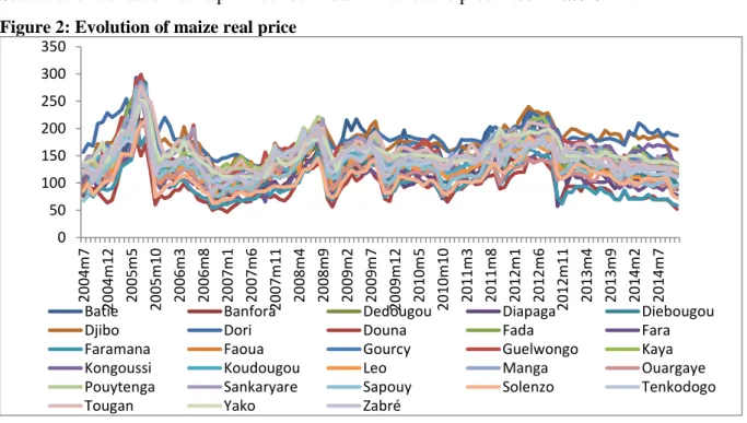
Figure 2: Evolution of maize real price
Source: SONAGESS and INSD
Figure 2 displays the evolution of real prices on the 28 maize markets. The price series
present similarities between markets, and notably important price spikes followed by price
10 Section 5.3 will make use of nominal price series in robustness checks.
0 50 100 150 200 250 300 350 20 04m 7 20 04m 12 20 05m 5 20 05m 10 20 06m 3 20 06m 8 20 07m 1 20 07 m 6 20 07m 11 20 08m 4 20 08m 9 20 09m 2 20 09m 7 20 09m 12 20 10m 5 20 10m 10 20 11m 3 20 11m 8 20 12m 1 20 12m 6 20 12m 11 20 13m 4 20 13m 9 20 14m 2 20 14m 7
Batie Banfora Dedougou Diapaga Diebougou
Djibo Dori Douna Fada Fara
Faramana Faoua Gourcy Guelwongo Kaya Kongoussi Koudougou Leo Manga Ouargaye Pouytenga Sankaryare Sapouy Solenzo Tenkodogo
11 drops in 2004/2005 (grasshopper invasion), 2007/2008 (drought and international crisis) and 2010/2011 (drought). Prices are affected by seasonal patterns: they are lower in the harvest season around October-December and higher in the lean period (June to September).
Figure 3: Localization of maize markets, main border crossing points11 and main cities
Source: Author calculation
The localization of each selected maize market is shown in Figure 3. Market remoteness is defined as market distance to main cities, namely Ouagadougou, Bobo-Dioulasso and Koudougou. Statistics pertaining to these three main cities are given in Table 1.
Table 1: Statistics related to main cities
Ouagadougou Bobo-Dioulasso Koudougou
Region Center Hauts-Bassins Centre-Ouest
Population 1.5 million 0.5 million 0.1 million
Population growth rate 7.6% 7.23% 3.4%
Source: Author calculation
11 Relying on the volume of maize trade, we identified four major maize border-crossing points (in red in Figure
3) among eighteen: Bittou (Togo), Dakola (Ghana), Léo (Ghana) and Niangoloko (Côte d’Ivoire). Figure 3 also plots the three main consumption centers in green.
12
4. Empirical strategy
We test the effect of market remoteness on price volatility. To do so, we use a pooling regression of 28 markets that permits an estimation of the average effect of market remoteness on maize price volatility. Our work focuses on the empirical analysis of price volatility, which is defined as the unpredictable component of price fluctuations (Prakash, 2011). Appropriate models for this measure of volatility are ARCH family models, in which the variance of residuals is allowed to depend on the most recent residuals and other variables.
Drawing on Shively (1996) , Barrett (1997) and Maître d’Hôtel et al. (2013), we build upon an ARCH model that displays mean and variance equations of maize prices to investigate maize price volatility in Burkina Faso. To measure this volatility, we isolate the unpredictable component of price variations from the predictable one, relying on price forecast models. To identify predictable price moves, several authors have used the conditional variance of price as an indicator of price volatility. The variance of the residuals of a price formation model typically measures the unpredictable price shifts. Thus, we use an ARCH model for two reasons. First, many storable commodity prices such as maize have an ARCH process (Beck,
1993). Second, ARCH models are particularly adaptable to the study of price volatility
defined as the unpredictable part of price variations, as they enable the variance of the residual not to be constant over time, thus depicting an unpredictable dimension. The ARCH model assumes that the conditional variance depends on the lagged squared residuals of a price series over time. By including variables as regressors, the model can be used to identify potential determinants of price volatility. The ARCH model was introduced by Engle (1982)
and generalized by Bollerslev (1986)12.
The ARCH structure is given by equations (12) and (13):
Yt = X′tβ + εt (11)
With εt|Ωt-1 ≈N (0,ht) (12)
12 A General Autoregressive Conditional Heteroskedasticity (GARCH) process can also model price volatility.
Some studies have used a GARCH model to analyse price volatility for different commodities (Yang et al., 2001 ; Gilbert and Morgan, 2010). We choose ARCH model instead of GARCH, because monthly data usually do not exhibit GARCH effects (Baillie and Bollerslev, 1990). GARCH model is more appropriate for high frequency data. A robustness check is conducted in section 5.3, which relies on GARCH model. By using ARCH and GARCH processes, we assume that a quadratic relationship between the error term and the conditional variance (i.e. volatility). Series are assumed to feature high and low volatility, whatever the sign of the shock causing the volatility. Other specifications called asymmetric models exist such as Exponential-ARCH (EGARCH) model, which has been used whether the price volatility depends on the information of past shock in a non-linear fashion. The asymmetric models assumes that volatility can be spotted with clusters of amplitudes that significantly vary over time and volatility can increase or decrease depending on the information on past error terms.
13
ht= ω+ ∑qi=1αiε²t−i (13)
where 𝑌𝑡 is the dependent variable, 𝑋′𝑡 denotes the vector of explanatory variables (column
vector), 𝜀𝑡 is the error component, ℎ𝑡 is the time-varying variance of the error; 𝛺t-1 is the
information set available at 𝑡 − 1, 𝜔, 𝛼𝑖 for i = 1,2,. . ., 𝛽 are parameters. Equation (11) gives
the conditional mean while equation (13) describes the evolution of the conditional variance. We adapt equations (11) and (13) to our study so as to investigate the determinants of maize price volatility in Burkina Faso.
We proceed in a two-step approach. Firstly, we pool 28 maize markets in order to estimate the
average effect of market remoteness (i.e. transport cost, time distance between market 𝑖 from
Ouagadougou, Bobo-Dioulasso and Koudougou: the major consumption centers) on price level (equation 14), and secondly, on price volatility (equation 15):
𝑙𝑛 𝑃𝑖𝑡 = 𝜃0+ 𝜃1𝑙𝑛 𝑃𝑖𝑡−1+ 𝜃2𝑇𝑟𝑒𝑛𝑑𝑡+ 𝜃3𝑙𝑛 𝑅𝐸𝑅𝑡+ 𝜃4𝑙𝑛𝐼𝑃𝑡+ ∑ µ𝑖 𝑖𝑆𝑖𝑡+ ∑ ʊ𝑗 𝑗𝑀𝑗ℎ+
𝜌𝑙𝑛𝑇𝐶 + 𝛿1𝑙𝑛𝐵𝑜𝑟𝑑𝑒𝑟 + 𝛿2𝑆𝑢𝑟𝑝𝑙𝑢𝑠 + 𝜀𝑖𝑡 (14)
ℎ𝑖𝑡 = 𝜆0+ 𝜆1ε2t−i+ 𝛺1𝑙𝑛 𝑃𝑖𝑡−1+ 𝛺2𝑇𝑟𝑒𝑛𝑑𝑡+ 𝛺3𝑙𝑛 𝑅𝐸𝑅𝑡+ 𝛺4𝑙𝑛𝐼𝑃𝑡+ ∑ 𝜋𝑖 𝑖𝑆ℎ𝑡+
𝜑𝑙𝑛𝑇𝐶 + 𝜔1𝑙𝑛𝐵𝑜𝑟𝑑𝑒𝑟 + 𝜔2𝑆𝑢𝑟𝑝𝑙𝑢𝑠 + 𝑣𝑖𝑡 (15)
The specifications retained indicate that explanatory variables have been introduced in both
mean and variance equations. 𝑳𝒏 𝑷𝒊𝒕 and 𝑳𝒏 𝑷𝒊𝒕−𝟏 are the natural logarithms of real maize
price in market 𝒊 at months 𝒕 and 𝒕 − 𝟏 respectively. 𝑻𝒓𝒆𝒏𝒅, 𝑹𝑬𝑹 and 𝑰𝑷 represent the
monthly trend, the real exchange rate13 and the international maize price respectively. 𝑺 refers
to seasonal14 dummy variables (lean and harvest seasons) while 𝑴 denotes maize market
dummy variables. 𝜺𝒊𝒕 is the error term. 𝑩𝒐𝒓𝒅𝒆𝒓 is a continuous variable that measures the
distance between market 𝑖 and the nearest cross-border maize point with Ghana, Côte
d’Ivoire, or Togo, four border points being considered because of their importance in terms of maize trade volumes. 𝑺𝒖𝒓𝒑𝒍𝒖𝒔 is a dummy variable which indicates whether the market is in surplus production area. 𝑺𝒖𝒓𝒑𝒍𝒖𝒔 equals 1 for maize-surplus regions and 0 for maize-deficit regions. In this study, we capture (TC) Transport Cost through three measures: time distance,
13 The real exchange rate and the real international price are computed as the ratio of the FCFA to the US dollar
and then deflated using the Burkinabe Consumer Price Index. We also use the natural logarithm to smooth the series.
14 In Burkina Faso, seasonal variability is characterized by differences in prices between the lean (June to
14
kilometric distance and road quality15. Transport Cost or Market remoteness can be defined
in various ways. The kilometric distance and travel time to a main urban center or a major market are the most commonly used measures (Barrett, 1996; Minten and Kyle, 1999;
Stifel and Minten, 2008; Minot, 2013). The quality of road infrastructure can be
alternatively used (Minten and Randrianarison, 2003) to have a more accurate measure of travel costs (time, gasoline).
In equations (14) and (15), 𝜌 tests whether the mean prices are different between remote
markets and markets close to the main urban centers, whereas 𝝋 tests to which extent maize
price series in remote markets are volatile. In accordance with the theoretical model in
equation 7, we expect maize prices to be lower in remote markets than in markets located
close to main consumption centers (𝝆 < 0). Based on equation 10, we expect 𝝋 > 0, i.e. remote markets exhibit greater maize price volatility than markets located close to main
consumption centers. The coefficient µ𝑖 tests the effect of seasonality on maize price level. In
accordance with equation 8, we expect low price levels in the harvest season (µ > 0) and high price levels in the lean season (µ < 0). In the case of maize-surplus markets, we should
have 𝛿2 <0 based on equation 6. Data source and descriptive statistics of all the variables
used in our study are presented in Appendix 5 and 6. The model is estimated in a system framework (with mean and variance equations) with Eviews 7 software. Our procedure is based on the maximum likelihood estimation method. Before starting the estimations, maize
price series, the dependent variable, was tested for stationarity. The Augmented Dickey Fuller
(ADF) for panel data was applied to test the null hypothesis of the presence of unit roots, following (Im et al., 2003). The panel unit root test leads to reject the null hypothesis of non-stationarity at the 5% level. The order of the ARCH model is determined through an assessment of the statistical significance generated from the Lagrange multiplier test. Results suggest that the price process is correctly described by an autoregressive order of one. The asymmetric (leverage) effect is investigated by examining whether the lagged values of standardized residuals influenced the price volatility. Results indicate that the price volatility is uncorrelated with the level of standardized residual, suggesting that there are no asymmetric effects; therefore, we do not need to apply an asymmetric model such as an EGARCH. Market dummy variables are omitted in the variance equation because dummy variables such as Surplus capture market characteristics.
15 Kilometric distance between a selected market and the nearest urban center and the road quality dummy
variable indicating whether the road leading to a market is paved or not are exclusively used in robustness checks (section 5.3) as alternatives measures of remoteness.
15
5. Empirical estimations
5.1 Spatial disparities in maize price volatility
Figure 4 presents the level of maize price volatility in each of the 28 Burkinabe markets over
2004-2013. It clearly suggests spatial differences in maize price volatility across markets. It appears that markets located far from the major consumption centers – Ouagadougou, Bobo-Dioulasso or Koudougou - register the highest levels of price volatility, thereby justifying our research question.
Figure 4: Differences spatial volatility of maize in Burkina Faso over 2004-2013
Source: Author calculation
5.2 Market remoteness as an explaining factor
We analyze the effect of time distance between a market and the nearest urban center on the volatility of the maize price prevailing in this market.
16
Table 2: The impact of market remoteness on price volatility
Variables Mean Equation Variance Equation Constant 4.0838*** (12.25) 0.0522*** (3.16) Ln Pt-1 0.9098*** (119.12) -0.0002 (0.00) ARCH(1) term 0.1095*** (5.87) Lean 0.0156*** (3.12) 0.0009*** (3.16) Harvest -0.0625*** (13.30) 0.0139*** (26.68) Trend -0.0003 (1.13) -0.0000*** (5.76) Exchange Rate 0.0744 (1.61) -0.0034 (1.65) International Price 0.0041 (0.18) -0.0017 (1.82) Time distance -0.0586*** (6.46) 0.0001*** (4.05) Border Surplus 0.0601** (2.57) -0.0890*** (3.19) -0.0004*** (3.28) 0.0016*** (5.60)
Markets Dummy YES NO
N R²
3163 0.8285 Notes: Values in parentheses are t-statistics
*** and ** denote significance at 1% and 5% levels, respectively.
Results from the ARCH model estimates from maximum likelihood estimation are found in
table 2. This table presents the results of the model fitted to 28 pooled maize markets.
Estimates of the mean equation indicate that price series follow an autoregressive process with a strong monthly autocorrelation. Results establish a seasonal pattern characterized by
low prices during the harvest time and high prices during the lean season16. These results are
16 Because of the existence of natural agricultural production cycles, agricultural prices are affected by
seasonality: indeed, there is an intra-annual price variation that tends to repeat regularly (Schnepf, 2005). Intra-annual agricultural price variations imply that prices are at their lower level in harvest time because of the abundance of products on markets but they progressively go up and are at their highest level just before the next harvest season.
17 consistent with our theoretical model and findings from many studies in the literature (Shively, 1996; Barrett, 1996; Jordaan et al., 2007; Kilima et al., 2008 and (Maître
d’Hôtel et al., 2013). On average, the level of maize price does not particularly increase over
time. We find that there is no significant effect of the exchange rate and international maize prices on price levels in Burkina Faso, suggesting that such external factors do not seem to influence price levels: maize prices are rather driven by domestic factors.
Coefficients on the spatial variables suggest that geographic location has an impact on the domestic price level with a 5% level of statistical significance. The results show that maize prices are lower in maize-surplus markets; this finding being consistent with Kilima et al.
(2008). Prices in maize-surplus markets are on average 8.9% lower than those prevailing in
maize-deficit markets. In these markets, supply exceeds demand, which drives the price down. The price of maize is also lower in markets close to the main maize border-crossing points. However, it is not easy to interpret this result. The price of maize in remote markets is 5,8% smaller than that observed in markets close to the main urban centers. It is worth noting that remote markets are not all net suppliers; those located in the north (Dori and Djibo) are typically net deficit markets. However, the majority of remote markets in our data appear to be net suppliers, implying on average lower maize prices. Furthermore, maize is the second-preferred crop (after rice) in main consumption centers. As these urban markets are located in low maize-production areas, demand exceeds supply, leading prices to be higher than in remote markets. This finding is consistent with the theoretical model that we have developed in equation 7, presented in section 2, which suggests that the price of food increases, as one gets closer to urban areas.
Estimates from the variance equation confirm that our model is correctly described by an ARCH model. The significance of the ARCH term indicates that price volatility depends on the past values of the residuals; this result is statistically significant at the 1% level. In
addition, seasonality17, trend and spatial position across markets have a significant effect on
price volatility: The effect of international prices and exchange rate on price volatility is non-significant. We also find that price volatility in Burkinabe maize markets has decreased over time. Spatial price volatility across markets is examined through time distance, maize border-crossing points and maize-surplus variables. Results indicate that coefficients on these
17 Results from the variance equation suggest that seasonality is an important component of maize price
18 variables are statistically significant at the 1% level. The positive parameter on Surplus suggests that prices in maize-surplus markets are more volatile than prices in maize-deficit markets. Previous findings also indicate that price volatility tends to be higher in maize-surplus markets than in maize-deficit markets (Kilima et al., 2008). The intuition is that a local supply shock arising on a maize-surplus market does not necessarily lead to a reduction in maize supply on this market through a transfer of quantities to maize-deficit regions, essentially because of the lack of sufficient market integration. This results in price volatility in maize-surplus markets. We also find that the coefficient on time distance to urban centers is significant. For example, results from the ARCH model indicate that on average remoteness from main consumption centers led to an increase of maize price volatility to 0,01%. The positive sign shows that remote markets tend to exhibit higher price volatility. Indeed, the urban center draws food production over the year, which ensures an adequate equilibrium between supply and local demand, thus stabilizing prices. This confirms the theoretical model we have been drawing in section 2, and the expected effects derived from equation (10). The negative and significant impact of border on price volatility indicates that prices in markets close to the main maize border-crossing points are more volatile than in other markets. The statistical significance of the coefficient on border - independently from the coefficient on remoteness - suggests that border captures additional information: market isolation should not only be comprehended as simple geographic remoteness from domestic urban centers. Remoteness is also expressed through high transport costs, export prohibitions and non-tariff barriers to crossing the border, which all hamper maize marketing abroad. Tackling remoteness by reducing or eliminating non-tariff barriers is essential to promoting regional integration and maize marketing in neighboring countries (Kaminski et al., 2013). Opening of borders is indeed crucial in reducing spatial price volatility and ultimately fostering food security in Burkina Faso (World Bank, 2012).
5.3 Robustness checks
The robustness of the previous results is tested in three ways. First, alternative measures of market remoteness are used; second, we carry out the same analysis with nominal price and lastly, we allow a change in the estimator used (GARCH model).
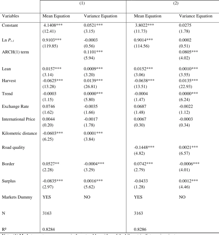
19 Alternative measure of market remoteness
Table 3: The impact of market remoteness on price volatility: Alternative measures of market remoteness
(1) (2)
Variables Mean Equation Variance Equation Mean Equation Variance Equation Constant 4.1408*** (12.41) 0.0521*** (3.15) 3.8022*** (11.73) 0.0275 (1.78) Ln Pt-1 0.9103*** (119.85) -0.0003 (0.56) 0.9014*** (114.56) 0.0002 (0.51) ARCH(1) term 0.1101*** (5.94) 0.0805*** (4.02) Lean 0.0157*** (3.14) 0.0009*** (3.20) 0.0152*** (3.06) 0.0010*** (3.55) Harvest -0.0625*** (13.28) 0.0139*** (26.81) -0.0638*** (13.51) 0.0135*** (22.93) Trend -0.0003 (1.15) 0.0000*** (5.80) -0.0004 (1.47) 0.0000*** (6.24) Exchange Rate 0.0746 (1.62) -0.0035 (1.66) 0.0687 (1.48) -0.0022 (1.12) International Price 0.0044 (0.20) -0.0017 (1.78) 0.0067 (0.30) -0.0003 (0.34) Kilometric distance -0.0603*** (6.25) 0.0001*** (3.84) Road quality -0.1448*** (4.82) 0.0021*** (6.57) Border 0.0527** (2.28) -0.0004*** (3.29) 0.0742*** (2.79) -0.0006*** (4.01) Surplus -0.0835*** (2.97) 0.0016*** (5.62) -0.0433 (1.28) 0.0012*** (4.46)
Markets Dummy YES NO YES NO
N 3163 3163
R² 0.8284 0.8286
Note: (1) Market remoteness measure is the natural logarithm of the kilometric distance in minutes. (2) Market remoteness measure is the dummy road quality
Values in parentheses are t-statistics
20 Two alternative measures of market remoteness are tested. The first measure is the distance in
kilometers18 between a selected market and the nearest main consumption center, the second
one is the quality of the road19 connecting the market with its main consumption center. Table
3 reports the results obtained. Columns (1) and (2) present the results obtained with the
kilometric distance and road quality, respectively.
In column (1), the finding that remote markets exhibit greater maize price volatility than markets located close to main consumption centers is confirmed again through the strongly positive coefficient on distance in kilometers. The same result holds in column (2) of table 3. Market remoteness proxied by unpaved road connected to the markets is positively and significantly associated with maize price volatility. The coefficient on the road quality is positive and statistically significant at the 1% level. The positive effect of market remoteness on maize price volatility in Burkina Faso holds for each of the three empirical specifications used.
Estimation with nominal price
We analyze our initial results with nominal price. We test whether our results are sensitive to price specification. Table 4 reports the results obtained. It indicates that even with nominal price series, the positive and significant impact of time distance on maize price volatility still holds and appears identical with the results obtained in table 2. Therefore, we show that the results are not sensitive to the functional form retained.
18 To compute information about kilometric distance, we relied on data from the Ministry of Agriculture,
specifically from the DGESS (Direction Générale des Etudes et des Statistiques Sectorielles) and data from google maps. We used DGESS data and resort to google maps to fill in for missing data due to the fact that information about some markets are not communicated by DGESS. However, it is reassuring to note that the DGESS data are comparable to data from google maps.
19 Road quality is equal to 1 if the national road connected to the selected market is unpaved, 0 otherwise. Road
21
Table 4: The impact of market remoteness on price volatility: estimation with nominal price
Variables Mean Equation Variance Equation Constant 0.4863 (0.82) 0.0037 (0.55) Ln Pt-1 0.8988*** (100.49) -0.0003 (0.71) ARCH(1) term CPI 0.8958 (16.23) 0.0986*** (9.53) 0.0032*** (6.28) Lean 0.0147*** (2.60) 0.0012*** (5.81) Harvest -0.0621*** (12.83) 0.0158*** (25.66) Trend -0.0005 (1.65) -0.0000*** (16.57) Exchange Rate -0.0470 (0.56) -0.0008 (0.58) International Price 0.0008 (0.03) -0.0004 (0.83) Time distance -0.0388*** (4.15) 0.0001*** (3.08) Border Production 0.1015** (4.46) -0.1228*** (4.73) -0.0004*** (4.00) 0.0017*** (7.28)
Markets Dummy YES NO
N R²
3163 0.8740
Notes: Values in parentheses are t-statistics
22 Estimation with GARCH model
An alternative specification to test the sensitivity of our results is implemented with the GARCH model. A number of studies have used a GARCH model to analyze maize price volatility (Gilbert and Morgan, 2010 ; Minot, 2013). In a GARCH model (Bollerslev,
1986), an autoregressive moving average (ARMA) model is assumed for the error variance. A
GARCH (p,q) model may be presented in the same manner as the ARCH model except that the variance equation is now as follows:
ht= ω + ∑qi=1𝜆iε²t−i+ ∑𝑝𝑗=1𝛽𝑗Ϭ²𝑡−𝑗 (16)
Non-negativity of the conditional variances requires ω, 𝜆i, βi > 0.
𝑙𝑛 𝑃𝑖𝑡 = 𝜃0+ 𝜃1𝑙𝑛 𝑃𝑖𝑡−1+ 𝜃2𝑇𝑟𝑒𝑛𝑑𝑡+ 𝜃3𝑙𝑛 𝑅𝐸𝑅𝑡+ 𝜃4𝑙𝑛𝐼𝑃𝑡+ ∑ µ𝑖 𝑖𝑆𝑖𝑡+ ∑ ʊ𝑗 𝑗𝑀𝑗ℎ+
𝜌𝑙𝑛𝑅𝑒𝑚𝑜𝑡𝑒 + 𝛿1𝑙𝑛𝐵𝑜𝑟𝑑𝑒𝑟 + 𝛿2𝑃𝑟𝑜𝑑𝑢𝑐𝑡𝑖𝑜𝑛 + 𝜀𝑖𝑡 (17)
ℎ𝑖𝑡 = 𝜆0+ 𝜆1ε2
t−i+ 𝛽1Ϭ²t−i+ 𝛺1𝑙𝑛 𝑃𝑖𝑡−1+ 𝛺2𝑇𝑟𝑒𝑛𝑑𝑡+ 𝛺3𝑙𝑛 𝑅𝐸𝑅𝑡+ 𝛺4𝑙𝑛𝐼𝑃𝑡+
∑ 𝜋𝑖 𝑖𝑆ℎ𝑡+ 𝜑𝑙𝑛𝑅𝑒𝑚𝑜𝑡𝑒 + 𝜔1𝑙𝑛𝐵𝑜𝑟𝑑𝑒𝑟 + 𝜔2𝑃𝑟𝑜𝑑𝑢𝑐𝑡𝑖𝑜𝑛 + 𝑣𝑖𝑡 (18)
The corresponding estimation is shown in table 5 which reports a significant and positive impact of market remoteness on maize price volatility, with similar findings for other variables. However, the coefficient associated with the GARCH model is non-significant. It is not easy to explain the non-significance of the GARCH term. One possibility is that monthly data usually do not exhibit GARCH effects (Baillie and Bollerslev, 1990). Even if a GARCH process exists, it will be due to the structural break of unconditional variance. Furthermore, GARCH application is more appropriate for high frequency data; however, in our application we use monthly data. Both ARCH and GARCH processes usually generate persistence in price volatility, i.e. high volatility is followed by high volatility, and the same holds for low volatility. The ARCH process features high persistence of price volatility but with short memory in that only the most recent residuals (shocks) have an impact on the current volatility. The GARCH model gives a much more smoothed volatility profile with long duration, in which past residuals and lagged volatility terms affect the current price volatility. This means that price volatility in Burkina Faso’s maize market is mainly due to recent shocks and the geographic situation within the country.
23
Table 5: The impact of market remoteness on price volatility: GARCH model
Variables Mean Equation Variance Equation Constant 4.0883*** (12.28) 0.0526*** (3.20) Ln Pt-1 0.9101*** (118.36) -0.0002 (0.42) ARCH(1) term GARCH(1) term 0.1115*** (5.92) 0.0059 (0.25) Lean 0.01558*** (3.10) 0.0009*** (3.21) Harvest -0.0628*** (13.11) 0.0139*** (26.71) Trend -0.0003 (1.14) -0.0000*** (5.65) Exchange Rate 0.0742 (1.61) -0.0035 (1.67) International Price 0.0039 (0.17) -0.0018 (1.88) Time distance -0.0585*** (6.42) 0.0001*** (3.97) Border Production 0.0600** (2.57) -0.0893*** (3.21) -0.0004*** (3.31) 0.0016*** (5.60)
Markets Dummy YES NO
N R²
3163 0.8285
Notes: Values in parentheses are t-statistics
24
6. Conclusion
The aim of this study was to examine the role of market remoteness in explaining maize price volatility in Burkina Faso over the period July 2004-November 2013. To reach this objective, we develop a model of price formation and transport costs between rural and urban markets and also captures the implications for price volatility in rural market. We explore the empirical implications of our conceptual model by using the autoregressive conditional heteroskedasticity (ARCH) model introduced by Engle (1982). The empirical estimations with data on 28 markets established that markets that are close to the main cities, where quality road infrastructure is available, display less volatile price series. The results also show that maize-surplus markets and markets bordering Côte d’Ivoire, Ghana and Togo have experienced more volatile prices than maize-deficit and non-bordering markets. Furthermore, we find strong evidence of a seasonal pattern in maize price volatility across Burkinabe markets.
These findings suggest that policies targeted towards infrastructure development and better regional integration and economic development within the ECOWAS area would reduce maize price volatility. For instance, authorities could support remote markets by linking them through better roads with major consumption centers across the country as well as in neighboring countries. This will be key to improve the commercialization of agricultural products in remote areas and reduce price volatility across markets in Burkina Faso.
References
Abdulai, A., 2000. Spatial price transmission and asymmetry in the Ghanaian maize market. J. Dev. Econ. 63, 327–349. doi:10.1016/S0304-3878(00)00115-2
Badiane, O., Shively, G.E., 1998. Spatial integration, transport costs, and the response of local prices to policy changes in Ghana. J. Dev. Econ. 56, 411–431. doi:10.1016/S0304-3878(98)00072-8
Baillie, R.T., Bollerslev, T., 1990. A multivariate generalized ARCH approach to modeling risk premia in forward foreign exchange rate markets. J. Int. Money Finance 9, 309– 324. doi:10.1016/0261-5606(90)90012-O
Barrett, C.B., 1996. On price risk and the inverse farm size-productivity relationship. J. Dev. Econ. 51, 193–215. doi:10.1016/S0304-3878(96)00412-9
Barrett, C.B., 1997. Liberalization and food price distributions: ARCH-M evidence from Madagascar. Food Policy 22, 155–173. doi:10.1016/S0306-9192(96)00033-4
Beck, S.E., 1993. A Rational Expectations Model of Time Varying Risk Premia in Commodities Futures Markets: Theory and Evidence. Int. Econ. Rev. 34, 149–168. doi:10.2307/2526954
Bollerslev, T., 1986. Generalized autoregressive conditional heteroskedasticity. J. Econom. 31, 307–327. doi:10.1016/0304-4076(86)90063-1
Deaton, A., Laroque, G., 1992. On the Behaviour of Commodity Prices. Rev. Econ. Stud. 59, 1–23. doi:10.2307/2297923
25 Engle, R.F., 1982. Autoregressive Conditional Heteroscedasticity with Estimates of the
Variance of United Kingdom Inflation. Econometrica 50, 987–1007.
doi:10.2307/1912773
Enke, S., 1951. A Equilibrium Among Spatially Separeted Markets: Solution by Electrical. Econometrica 19, 40–47.
Fafchamps, M., 1992. Cash Crop Production, Food Price Volatility, and Rural Market Integration in the Third World. Am. J. Agric. Econ. 74, 90–99. doi:10.2307/1242993 Gilbert, C.L., Morgan, C.W., 2010. Food price volatility. Philos. Trans. R. Soc. B Biol. Sci.
365, 3023–3034. doi:10.1098/rstb.2010.0139
Im, K.S., Pesaran, M.H., Shin, Y., 2003. Testing for unit roots in heterogeneous panels. J. Econom. 115, 53–74. doi:10.1016/S0304-4076(03)00092-7
Jordaan, H., Grové, B., Jooste, A., Alemu, Z.G., 2007. Measuring the Price Volatility of Certain Field Crops in South Africa using the ARCH/GARCH Approach. Agrekon 46, 306–322. doi:10.1080/03031853.2007.9523774
Kaminski, J., Christiaensen, L., Gilbert, C.L., 2014. The end of seasonality ? new insights from Sub-Saharan Africa (Policy Research Working Paper Series No. 6907). The World Bank.
Kaminski, J., ELBEHRI, A., ZOMA, J.-B., 2013. Analyse de la filière du maïs et compétitivité au Burkina Faso: politiques et initiatives d’intégration des petits producteurs au Marché
Kilima, F.T.M., Chanjin, C., Phil, K., Emanuel R, M., 2008. Impacts of Market Reform on Sptial Volatility of Maize Prices in Tanzania. J. Agric. Econ. 59, 257–270. doi:10.1111/j.1477-9552.2007.00146.x
Maître d’Hôtel, E., Le Cotty, T., Jayne, T., 2013. Trade Policy Inconsistency and Maize Price Volatility: An ARCH Approach in Kenya. Afr. Dev. Rev. 25, 607–620. doi:10.1111/1467-8268.12055
Minot, N., 2014. Food price volatility in sub-Saharan Africa: Has it really increased? Food Policy 45, 45–56.
Minten, B., Kyle, S., 1999. The effect of distance and road quality on food collection, marketing margins, and traders’ wages: evidence from the former Zaire. J. Dev. Econ. 60, 467–495.
Minten, B., Randrianarison, L., 2003. Etude sur la Formation des prix du Riz Local à Madagascar.
Piot-Lepetit, I., Mbarek, R., 2011. Methods to analyze agricultural commodity price volatility, Springer. ed.
Prakash, A., 2011. Safeguarding food security in volatile global markets. xxii + 594 pp. Samuelson, P.A., 1952. Spatial price equilibrium and linear programming. Am. Econ. Rev.
283–303.
Schnepf, R.D., 2005. Price determination in agricultural commodity markets: A primer. Congressional Research Service, Library of Congress.
Shively, G.E., 1996. Food Price Variability and Economic Reform: An ARCH Approach for Ghana. Am. J. Agric. Econ. 78, 126–136. doi:10.2307/1243784
Stifel, D., Minten, B., 2008. Isolation and agricultural productivity. Agric. Econ. 39, 1–15. doi:10.1111/j.1574-0862.2008.00310.x
World Bank, 2012. Africa Can Help Feed Africa/ Document Removing barriers to regional
trade in food staples/ The World Bank
Yang, J., Haigh, M.S., Leatham, D.J., 2001. Agricultural liberalization policy and commodity price volatility: a GARCH application. Appl. Econ. Lett. 8, 593–598. doi:10.1080/13504850010018734
26
A1: Evolution of millet, maize, rice and sorghum production in Burkina Faso since 1961
Source: FAO, Data viewed on January 06, 2015
0 500000 1000000 1500000 2000000 2500000 Millet Maize Rice Sorghum
27
A2: Evolution of maize production in Burkina Faso since 1984 (tons)
Source: COUNTRYSTAT data downloaded on July 05, 2013
0 50000 100000 150000 200000 250000 300000 350000 400000 450000 1984 1986 1988 1990 1992 1994 1996 1998 2000 2002 2004 2006 2008 2010 Boucle Du Mouhoun Cascades Centre Centre-est Centre-nord Centre-ouest Centre-sud Est Hauts-bassins Nord Plateau Central Sahel Sud-ouest
28
A3: Map of maize production in 2011
29
A4: Descriptive statistics of the prices observed in each market
Number of Observations Mean Standard deviation Min Max Banfora 113 83.86 19.27 49.99 151.42 Batié 113 102.33 23.45 54.35 197.29 Dédougou 113 92.29 21.75 58.74 178.68 Diapaga 113 87.30 25.40 35.46 178.61 Diébougou 113 89.99 24.13 55.02 199.76 Djibo 113 119.57 17.21 83.81 176.88 Dori 113 123.79 21.26 95.81 205.08 Douna 113 64.65 17.28 36.17 121.23 Fada 113 99.56 22.96 60.28 184.23 Fara 113 74.83 17.78 42.56 140.97 Faramana 113 68.81 19.17 37.83 142.20 Gaoua 113 103.55 17.39 64.66 175.84 Gourcy 113 109.64 16.58 85.49 166.19 Guelwongo 113 109.20 21.47 73.28 204.69 Kaya 113 107.86 18.40 81.14 174.82 Kongoussi 113 102.54 18.45 72.12 178.26 Koudougou 113 100.12 19.53 68.26 173.39 Léo 113 91.21 20.75 56.47 175.48 Manga 113 103.41 21.86 66.74 195.57 Ouargaye 113 81.32 17.75 47.36 145.48 Pouytenga 113 106.17 16.23 80.34 169.71 Sankaryaré 113 108.39 20.06 78.40 191.04 Sapouy 113 88.927 22.75 50.95 182.52 Solenzo 113 75.80 19.76 46.38 146.83 Tenkodogo 113 98.27 17.41 72.22 173.60 Tougan 113 108.82 20.14 74.62 190.86 Yako 113 106.49 17.93 80.19 172.77 Zabré 113 99.61 19.31 60.91 169.44
30
A5: Explanatory variables used
Variable name Type of variable Unit Source
𝑃𝑖𝑡 Real price Continuous FCFA/kg SONAGESS
𝑃𝑖𝑡−1 Lagged real price Continuous FCFA/kg SONAGESS
𝑅𝐸𝑅𝑡 Real exchange rate Continuous FCFA/USD IMF database
𝐼𝑃𝑡 Real international Price of Maize Continuous FCFA/kg IMF database
TC Time and kilometer distance between local market and main consumption center
Continuous Minutes
Google maps
Border Time distance between local market and main border crossing points
Continuous Minutes countrystat
Surplus Surplus of production Dummy 1(Surplus of
production)/0
Countrystat
31
A6: Descriptive statistics
Variable Obs Mean Std. Dev. Min Max
Real Price 3164 96.73006 24.50788 35.46873 205.46873
Trend 3164 57 32.62417 1 113
Real exchange Rate 3164 353.4873 69.90379 253.5087 513.5203
Real international price of maize 3164 64838.47 16633.54 39751.56 100274.8
TC 3164 141.8214 81.19211 0 374