Experimental validation of an optimized signal processing method to handle non-linearity in swept-source optical coherence tomography

(1)

Publisher’s version / Version de l'éditeur:

Optics Express, 18, 10, pp. 10446-10461, 2010-05-05

READ THESE TERMS AND CONDITIONS CAREFULLY BEFORE USING THIS WEBSITE.

https://nrc-publications.canada.ca/eng/copyright

Vous avez des questions? Nous pouvons vous aider. Pour communiquer directement avec un auteur, consultez la première page de la revue dans laquelle son article a été publié afin de trouver ses coordonnées. Si vous n’arrivez pas à les repérer, communiquez avec nous à PublicationsArchive-ArchivesPublications@nrc-cnrc.gc.ca.

Questions? Contact the NRC Publications Archive team at

PublicationsArchive-ArchivesPublications@nrc-cnrc.gc.ca. If you wish to email the authors directly, please see the first page of the publication for their contact information.

NRC Publications Archive

Archives des publications du CNRC

This publication could be one of several versions: author’s original, accepted manuscript or the publisher’s version. / La version de cette publication peut être l’une des suivantes : la version prépublication de l’auteur, la version acceptée du manuscrit ou la version de l’éditeur.

For the publisher’s version, please access the DOI link below./ Pour consulter la version de l’éditeur, utilisez le lien DOI ci-dessous.

https://doi.org/10.1364/OE.18.010446

Access and use of this website and the material on it are subject to the Terms and Conditions set forth at

Experimental validation of an optimized signal processing method to

handle non-linearity in swept-source optical coherence tomography

Vergnole, Sébastien; Lévesque, Daniel; Lamouche, Guy

https://publications-cnrc.canada.ca/fra/droits

L’accès à ce site Web et l’utilisation de son contenu sont assujettis aux conditions présentées dans le site LISEZ CES CONDITIONS ATTENTIVEMENT AVANT D’UTILISER CE SITE WEB.

NRC Publications Record / Notice d'Archives des publications de CNRC:

https://nrc-publications.canada.ca/eng/view/object/?id=f93f6264-749e-4ed1-bd79-831db7fbfe9e https://publications-cnrc.canada.ca/fra/voir/objet/?id=f93f6264-749e-4ed1-bd79-831db7fbfe9e

(2)

Experimental validation of an optimized signal

processing method to handle non-linearity in

swept-source optical coherence tomography

Sébastien Vergnole,* Daniel Lévesque, and Guy Lamouche

Industrial Materials Institute, National Research Council Canada, 75 Boulevard de Mortagne, Boucherville, QC, J4B 6Y4, Canada

*Sebastien.Vergnole@cnrc-nrc.gc.ca

Abstract: We evaluate various signal processing methods to handle the

non-linearity in wavenumber space exhibited by most laser sources for swept-source optical coherence tomography. The following methods are compared for the same set of experimental data: non-uniform discrete Fourier transforms with Vandermonde matrix or with Lomb periodogram, resampling with linear interpolation or spline interpolation prior to fast-Fourier transform (FFT), and resampling with convolution prior to FFT. By selecting an optimized Kaiser-Bessel window to perform the convolution, we show that convolution followed by FFT is the most efficient method. It allows small fractional oversampling factor between 1 and 2, thus a minimal computational time, while retaining an excellent image quality.

OCIS codes: (170.4500) Optical coherence tomography; (070.4340) Nonlinear optical signal

processing.

References and links

1. A. F. Fercher, C. K. Hitzenberger, G. Kamp, and S. Y. El Zaiat, “Measurement of intraocular distances by backscattering spectral interferometry,” Opt. Commun. 117(1-2), 43–48 (1995).

2. G. Häusler, and M. W. Linduer, ““Coherence radar” and “spectral radar”-new tools for dermatological diagnosis,” J. Biomed. Opt. 3(1), 21–31 (1998).

3. Z. Hu, and A. M. Rollins, “Fourier domain optical coherence tomography with a linear-in-wavenumber spectrometer,” Opt. Lett. 32(24), 3525–3527 (2007).

4. G. V. Gelikonov, V. M. Gelikonov, and P. A. Shilyagin, “Linear wave-number spectrometer for spectral domain optical coherence tomography,” Proc. SPIE 6847, 68470N (2008).

5. V. Gelikonov, G. Gelikonov, and P. Shilyagin, “Linear-wavenumber spectrometer for high-speed spectral-domain optical coherence tomography,” Opt. Spectrosc. 106(3), 459–465 (2009).

6. C. M. Eigenwillig, B. R. Biedermann, G. Palte, and R. Huber, “K-space linear Fourier domain mode locked laser and applications for optical coherence tomography,” Opt. Express 16(12), 8916–8937 (2008),

http://www.opticsinfobase.org/oe/abstract.cfm?URI=oe-16-12-8916.

7. D. C. Adler, Y. Chen, R. Huber, J. Schmitt, J. Connolly, and J. G. Fujimoto, “Three-dimensional endomicroscopy using optical coherence tomography,” Nat. Photonics 1(12), 709–716 (2007).

8. M. A. Choma, K. Hsu, and J. A. Izatt, “Swept source optical coherence tomography using an all-fiber 1300-nm ring laser source,” J. Biomed. Opt. 10(4), 044009 (2005).

9. B. A. Bower, M. Zhao, R. J. Zawadzki, and J. A. Izatt, “Real-time spectral domain Doppler optical coherence tomography and investigation of human retinal vessel autoregulation,” J. Biomed. Opt. 12(4), 041214–041218 (2007).

10. E. Götzinger, M. Pircher, R. A. Leitgeb, and C. K. Hitzenberger, “High speed full range complex spectral domain optical coherence tomography,” Opt. Express 13(2), 583–594 (2005),

11. M. Szkulmowski, M. Wojtkowski, T. Bajraszewski, I. Gorczynska, P. Targowski, W. Wasilewski, A. Kowalczyk, and C. Radzewicz, “Quality improvement for high resolution in vivo images by spectral domain optical coherence tomography with supercontinuum source,” Opt. Commun. 246(4-6), 569–578 (2005). 12. B. Cense, N. A. Nassif, T. C. Chen, M. C. Pierce, S.-H. Yun, B. H. Park, B. Bouma, G. Tearney, and J. de Boer,

“Ultrahigh-resolution high-speed retinal imaging using spectral-domain optical coherence tomography,” Opt. Express 12(11), 2435–2447 (2004), http://www.opticsinfobase.org/oe/abstract.cfm?URI=oe-12-11-2435. 13. C. Dorrer, N. Belabas, J.-P. Likforman, and M. Joffre, “Spectral resolution and sampling issues in

Fourier-transform spectral interferometry,” J. Opt. Soc. Am. B 17(10), 1795–1802 (2000).

(3)

14. S. H. Yun, G. J. Tearney, B. E. Bouma, B. H. Park, and J. F. de Boer, “High-speed spectral-domain optical coherence tomography at 1.3 mum wavelength,” Opt. Express 11(26), 3598–3604 (2003),

15. Y. Yasuno, V. D. Madjarova, S. Makita, M. Akiba, A. Morosawa, C. Chong, T. Sakai, K.-P. Chan, M. Itoh, and T. Yatagai, “Three-dimensional and high-speed swept-source optical coherence tomography for in vivo investigation of human anterior eye segments,” Opt. Express 13(26), 10652–10664 (2005),

16. N. A. Nassif, B. Cense, B. H. Park, M. C. Pierce, S. H. Yun, B. Bouma, G. Tearney, T. Chen, and J. de Boer, “In vivo high-resolution video-rate spectral-domain optical coherence tomography of the human retina and optic nerve,” Opt. Express 12(3), 367–376 (2004), http://www.opticsinfobase.org/oe/abstract.cfm?URI=oe-12-3-367. 17. A. R. Tumlinson, B. Hofer, A. M. Winkler, B. Považay, W. Drexler, and J. K. Barton, “Inherent homogenous

media dispersion compensation in frequency domain optical coherence tomography by accurate k-sampling,” Appl. Opt. 47(5), 687–693 (2008).

18. T. Endo, Y. Yasuno, S. Makita, M. Itoh, and T. Yatagai, “Profilometry with line-field Fourier-domain interferometry,” Opt. Express 13(3), 695–701 (2005), http://www.opticsinfobase.org/oe/abstract.cfm?URI=oe-13-3-695.

19. B. Baumann, E. Götzinger, M. Pircher, and C. K. Hitzenberger, “Single camera based spectral domain polarization sensitive optical coherence tomography,” Opt. Express 15(3), 1054–1063 (2007), http://www.opticsinfobase.org/oe/abstract.cfm?URI=oe-15-3-1054.

20. C. Fan, Y. Wang, and R. K. Wang, “Spectral domain polarization sensitive optical coherence tomography achieved by single camera detection,” Opt. Express 15(13), 7950–7961 (2007),

21. M. A. Choma, M. V. Sarunic, C. Yang, and J. A. Izatt, “Sensitivity advantage of swept source and Fourier domain optical coherence tomography,” Opt. Express 11(18), 2183–2189 (2003),

22. R. A. Leitgeb, W. Drexler, A. Unterhuber, B. Hermann, T. Bajraszewski, T. Le, A. Stingl, and A. F. Fercher, “Ultrahigh resolution Fourier domain optical coherence tomography,” Opt. Express 12(10), 2156–2165 (2004), http://www.opticsinfobase.org/oe/abstract.cfm?URI=oe-12-10-2156.

23. M. Wojtkowski, V. J. Srinivasan, T. H. Ko, J. G. Fujimoto, A. Kowalczyk, and J. S. Duker, “Ultrahigh-resolution, high-speed, Fourier domain optical coherence tomography and methods for dispersion compensation,” Opt. Express 12(11), 2404–2422 (2004),

24. Y. T. Pan, Q. Wu, Z. G. Wang, P. R. Brink, and C. W. Du, “High-resolution imaging characterization of bladder dynamic morphophysiology by time-lapse optical coherence tomography,” Opt. Lett. 30(17), 2263–2265 (2005). 25. H. Ren, T. Sun, D. J. MacDonald, M. J. Cobb, and X. Li, “Real-time in vivo blood-flow imaging by

moving-scatterer-sensitive spectral-domain optical Doppler tomography,” Opt. Lett. 31(7), 927–929 (2006). 26. P. Bu, X. Wang, and O. Sasaki, “Full-range parallel Fourier-domain optical coherence tomography using

sinusoidal phase-modulating interferometry,” J. Opt. A, Pure Appl. Opt. 9(4), 422–426 (2007).

27. T. S. Ralston, D. L. Marks, P. S. Carney, and S. A. Boppart, “Interferometric synthetic aperture microscopy,” Nat. Phys. 3(2), 129–134 (2007).

28. Y. Chen, H. Zhao, and Z. Wang, “Investigation on spectral-domain optical coherence tomography using a tungsten halogen lamp as light source,” Opt. Rev. 16(1), 26–29 (2009).

29. A. Liu, R. Wang, K. L. Thornburg, and S. Rugonyi, “Efficient postacquisition synchronization of 4-D nongated cardiac images obtained from optical coherence tomography: application to 4-D reconstruction of the chick embryonic heart,” J. Biomed. Opt. 14(4), 044020–044011 (2009).

30. R. Huber, M. Wojtkowski, K. Taira, J. Fujimoto, and K. Hsu, “Amplified, frequency swept lasers for frequency domain reflectometry and OCT imaging: design and scaling principles,” Opt. Express 13(9), 3513–3528 (2005), http://www.opticsinfobase.org/oe/abstract.cfm?URI=oe-13-9-3513.

31. B. Hofer, B. Považay, B. Hermann, A. Unterhuber, G. Matz, F. Hlawatsch, and W. Drexler, “Signal post processing in frequency domain OCT and OCM using a filter bank approach,” Proc. SPIE 6443, 64430O (2007). 32. S. S. Sherif, C. Flueraru, Y. Mao, and S. Change, “Swept Source Optical Coherence Tomography with

Nonuniform Frequency Domain Sampling,” in Biomedical Optics, OSA Technical Digest (CD) (Optical Society of America, 2008), paper BMD86.

33. T. H. Chow, S. G. Razul, B. K. Ng, G. Ho, and C. B. A. Yeo, “Enhancement of Fourier domain optical coherence tomorgraphy images using discrete Fourier transform method,” Proc. SPIE 6847, 68472T (2008). 34. K. Wang, Z. Ding, T. Wu, C. Wang, J. Meng, M. Chen, and L. Xu, “Development of a non-uniform discrete

Fourier transform based high speed spectral domain optical coherence tomography system,” Opt. Express 17(14), 12121–12131 (2009), http://www.opticsinfobase.org/oe/abstract.cfm?URI=oe-17-14-12121.

35. D. Hillmann, G. Huttmann, and P. Koch, “Using nonequispaced fast Fourier transformation to process optical coherence tomography signals,” Proc. SPIE 7372, 73720R (2009).

36. Y. Zhang, X. Li, L. Wei, K. Wang, Z. Ding, and G. Shi, “Time-domain interpolation for Fourier-domain optical coherence tomography,” Opt. Lett. 34(12), 1849–1851 (2009).

37. I. Gohberg, and V. Olshevsky, “Fast algorithms with preprocessing for matrix-vector multiplication problems,” J. Complexity 10(4), 411–427 (1994).

38. V. V. Vityazev, “Time series analysis of unequally spaced data: Intercomparison between the Schuster periodogram and the LS-spectra,” Astron. Astrophys. Trans. 11(2), 139–158 (1996).

39. N. R. Lomb, “Least-squares frequency analysis of unequally spaced data,” Astrophys. Space Sci. 39(2), 447–462 (1976).

(4)

40. W. H. Press, S. A. Teukolsky, W. T. Vetterling, and B. P. Flannery, Numerical Recipes in FORTRAN (Cambridge University Press, New York, 1992).

41. P. N. Swarztrauber, Vectorizing the FFTs, in Parallel Computations, G. Rodrigue, ed. (Academic Press, New York, NY, 1982), pp. 51–83.

42. M. Frigo, and S. G. Johnson, “FFTW: an adaptive software architecture for the FFT,” in Proceedings of IEEE

International Conference on Acoustics, Speech and Signal Processing. (Institute of Electrical and Electronics

Engineers, Seattle, 1998), pp. 1381–1384.

43. J. I. Jackson, C. H. Meyer, D. G. Nishimura, and A. Macovski, “Selection of a convolution function for Fourier inversion using gridding computerised tomography application,” IEEE Trans. Med. Imaging 10(3), 473–478 (1991).

44. P. J. Beatty, D. G. Nishimura, and J. M. Pauly, “Rapid gridding reconstruction with a minimal oversampling ratio,” IEEE Trans. Med. Imaging 24(6), 799–808 (2005).

45. C.-É. Bisaillon, G. Lamouche, R. Maciejko, M. Dufour, and J.-P. Monchalin, “Deformable and durable phantoms with controlled density of scatterers,” Phys. Med. Biol. 53(237–N), 247 (2008).

1. Introduction

In Fourier-domain optical coherence tomography (FD-OCT) [1, 2], the signal is collected as a function of the wavelength and the spatial information is recovered by a discrete Fourier transform (DFT). To maximize the image quality, the basic DFT requires to be performed with equally-spaced data in wavenumber space (k-space). Unfortunately, these digitized data are not commonly recorded with such a regular spacing in wavenumber. Various approaches have been developed to overcome this issue in the two branches of FD-OCT. These approaches involve hardware modifications: linear-wavenumber spectrometers have been developed [3–5] for spectral domain OCT (SD-OCT) and the feasibility of a linear-wavenumber swept source has been demonstrated for swept-source OCT (SS-OCT) [6]. Another solution in SS-OCT is to use an external k-trigger [7, 8]. This feature is available as an option on some commercial swept sources but it increases the total cost of the setup and the complexity of the data acquisition system.

However, a software solution is generally used. Several signal processing methods have been considered, most of them involving resampling the data at a regular interval in k-space and then applying the Fast Fourier Transform (FFT). The easiest way for data resampling is to perform a basic linear interpolation [9–12], but this technique usually leads to poor results. Some improvement is obtained by resampling the data with a smaller interval, i.e. with an oversampling factor of 2 or more. Alternatively, an interpolation method was proposed consisting in zero-filling the array after FFT of the raw data and then performing the inverse FFT back in the k-space. The new data are then linearly interpolated with a finer sampling [13–20]. Yasuno et al. [15] compared qualitatively these two techniques and showed that the zero-filling interpolation was about 10 times slower than the basic linear interpolation. The most popular resampling technique is the cubic spline interpolation used in a wide variety of papers in FD-OCT [21–28]. This technique is even perceived as the one “which offers the best cost-performance tradeoff among available interpolation methods” [29]. Other methods were proposed, such as the nearest-neighbor-check algorithm [30] to minimize time processing or the filter bank technique [31] which requires a special calibration and has only been applied to SD-OCT.

Very recently, non-uniform DFT algorithms have been used [32–35]. The most direct approach is the method which relies on the Vandermonde matrix first proposed in OCT by Sherif et al. [32]. A similar method called Schuster periodogram has been proposed in FD-OCT [33]. Finally, Hillmann et al. [35] proposed a method where resampling is done via a convolution of the data with a Kaiser-Bessel window prior to performing a FFT. This method is well known in the magnetic resonance imaging (MRI) community as the gridding method. Reference [35] suggests that this method is very efficient, although the demonstration is made only on simulated data in absence of noise. A similar convolution approach was proposed by Zhang et al. [36] with a kernel in the k-space equivalent to the zero-filling interpolation described above.

In this paper, we present a comparison of the different methods that can be used in SS-OCT. To provide a true assessment of the performance of the various methods, the comparison is not made with simulated data but with experimental data. Although SS-OCT is

(5)

used in this work, the results also apply to SD-OCT. We briefly review the selected methods which include non-uniform DFT with Vandermonde matrix or with Lomb periodogram, resampling with linear interpolation or spline interpolation prior to FFT, and resampling with convolution prior to FFT. For the latter, the convolution is performed with a Kaiser-Bessel window as proposed in Ref [35]. We introduce an improved implementation of the convolution method by using an optimized Kaiser-Bessel window that allows achieving good image quality with minimal computational time. Experimental data are then processed using each method to compare computational times and image quality by evaluating the point spread functions. Finally, we show images of a phantom and of a finger nail obtained with the different methods to better appreciate their performance. All these results do confirm that the most efficient method is the convolution with an optimized Kaiser-Bessel window followed by FFT.

2. Signal processing methods

The methods described below require an accurate calibration vector for the swept-laser source used, so that the wavenumber k=2π/λ is a priori known for all time sampling points, N. These methods are non-uniform discrete Fourier transform (DFT), resampling with interpolation followed by FFT, and resampling with convolution followed by FFT. Practical considerations for the implementation of each algorithm are given.

2.1 Non-uniform DFT

The most direct method to the problem is the use of a non-uniform DFT relying on the Vandermonde matrix [32]. The measured OCT signal in k-space Uk and the OCT profile in

spatial space un are linked by a Fourier transform that can be written as:

2 1 0 , N _i _k n N k n k k n U u e       



 (1)

In the above expression for the classical DFT, the k values are integers (i.e. non-dimensional wavenumber) and the k are evenly distributed on a unit circle in the complex plane. A

non-uniform DFT can be defined for k non-evenly spaced, i.e. where k values are not integers.

Also, this equation can be written in a matrix form as Uk D un, where D is a Vandermonde

matrix that can be inverted to relate the SS-OCT signal Uk measured with non-uniform

sampling in k-space to the OCT profile as 1

n k

u D U . To avoid any numerical instability in computing D1, one can use the forward transform instead, with summation over k values in the form: † n n k k k k u 



u  D U (2)

where the conjugate-transposed matrix D† is:

1 1 1 0 1 1 † 1 1 1 0 1 1 1 1 ... 1 ... _N N N N N D                              (3)

Rescaling with the k vector in the range kmin<k<kmax, the k in discrete form above are now expressed as: min ( ) i k k k e   _  z (4) with the step size in optical path length given by:

(6)

max min 2 (k k )     z (5)

Such a matrix can be calculated and stored once for processing all OCT signals. Alternatively, it can be calculated by row in a recursive manner for vector multiplication with the OCT signals of a B-scan each time at negligible computational costs. While the matrix-vector multiplication involved O(N2) operations, sophisticated algorithms exist to perform the task in O(N log2N) operations [37]. Since other approaches in this paper have a complexity O(N log N), there is no interest in further optimizing the Vandermonde matrix method and

this more exact method is only used as a reference. Also in the literature related to the power spectrum evaluation of a time series, this method is called the Schuster periodogram [33, 38].

The Lomb periodogram is another DFT for processing OCT signals that circumvents the resampling issue. Basically, such a method attributed to Lomb [39] was developed for estimating the power spectrum of a time series. The method uses a least-square fitting of a sinusoid to the data for each frequency and has a well-defined statistical behavior. Starting with a zero-mean time series un = u(tn) of N points with variance

2

 , the Lomb periodogram, function of the angular frequency0, is defined as [40]:

2 2 2 2 2 2 cos ( ) sin ( ) 1 ( ) , 2 cos ( ) sin ( ) n n n n n n n n n n u t u t U t t           _ _ _ _    _ _ _ _         _  _       



(6)

where   ω( )is an offset that makes the periodogram invariant to time translation as given by: sin 2 tan 2 . cos 2 n n n n t t    



(7)

Such a method can be used to process SS-OCT data in the k-space since inverse or direct

Fourier transform is equivalent. As a periodogram however, only the magnitude or the envelope is obtained, that is as a function of the optical path z (related to the variable ω) from unevenly sampled wavenumbers k (related to the variable t). A direct implementation of the

Lomb periodogram requires O(N2) operations. However, one can implement a fast algorithm of complexity O(N log N) for its evaluation to any desired degree of approximation by

spreading each measured point onto L most nearly centered mesh points using Lagrange

interpolating polynomials [40]. The number of points L is at least 2 and has a direct impact on

the computational time. The algorithm also uses FFT, but it is not for calculation of the DFT from the OCT data. Further optimization can be made toward a preprocessing step followed by the calculation only required for each OCT signal. The data windowing, e.g. using a Hamming window, is also allowed to reduce spectral leakage taking into account the measured point locations.

2.2 Interpolation with FFT

The most popular method to process the SS-OCT data is to first resample the data at regular interval in the k-space and then perform a conventional FFT. With the k vector in the range kmin<k<kmax, the step sizes in wavenumber domain δk and path length domain δz are given by:

max min max min ( ) 2 2 , ' ( ) k k k N N k k            z z (8)

(7)

where α is the oversampling factor in the k-space and N’=Nα is the number of points involved in the FFT operation. The value of α is a tradeoff between the accuracy and computational time, and is commonly set to 2. In our implementation, the FFT algorithm used only requires that N’ is the product of small prime numbers, possibly after padding the vector with a few

zeroes. Our implementation relies on the algorithm FFTPack [41], but a more sophisticated algorithm exists with a speedup factor of about 2 [42]. The windowing on resampled data with fixed step size is also allowed to reduce spectral leakage. For computational costs, the overall scheme has a complexity of O(N’ log N’).

Using the basic linear interpolation, the resampling is made on Nα values of k with the relation: ( ), k k k k k k k k U U w U U w k k             (9)

where k - and k + are the neighboring points on each side of k, and the wk are calculated once before processing all OCT signals. The result after the FFT operation usually shows a strong decrease with depth that should not be considered the actual sensitivity roll-off. In fact, the weighted average on each resampled point can be seen as a convolution with a triangle function [35]. The width of this triangle function is nevertheless not constant due to the nonlinearity of the data in k-space. Therefore, a correction can be applied by assuming that the data is convolved with an average window. Such a correction is applied after the FFT operation by multiplying the result with the vector cn defined as:

2 2 ( / ) sin ( / ) n n N c n N    (10)

Alternatively, the cubic spline interpolation involves U and its second derivative U” also

from nearest neighbor points, as given by [40]:

'' '' k k k k k k k k k U a U b U   f U  g U  (11) where: a_k  1 w_k, b_k w_k, 1 3 2 6( )( ) k k k f  a a kk and 1 3 2 6( )( ) k k k g  b b kk .

Its implementation requires the calculation of the second derivative of each OCT signal which makes the resampling more time consuming. Also, such a nearest neighbor calculation on each interpolated point requires a correction after the FFT operation which depends on the nonlinearity of the swept-laser source used, which can be determined empirically. This is made once by comparing the amplitude roll-off as a function of optical path with that of the reference method using the Vandermonde matrix, providing a vector cn as a polynomial fit:

( )j

n j

j

c 



d nz (12)

where the dj’s are the polynomial coefficients.

Another interpolation scheme has been proposed which is known as the zero-filling method. The standard FFT is first applied to the raw OCT data, the result is then filled with zeroes to a length typically 4N or 8N, and the FFT back into the k-space yields a vector with a

finer sampling and proper data interpolation. Although this scheme uses only FFT, it requires larger vectors to handle and makes the method much slower than the above two interpolation methods [15]. Thus, the zero-filling method is not further considered in this paper.

2.3 Convolution with FFT

A method, known as gridding in MRI, can be advantageously used for the data processing of the SS-OCT data [43]. In this method, OCT data is resampled by convolution in the k-space

with a finite window function as the kernel, followed by the use of conventional FFT. Very recently, such a method was proposed in OCT using a function with cosines, equivalent to the

(8)

zero-filling interpolation above [36], or using a Kaiser-Bessel function [35]. The approach uses the same oversampling factor α as for the interpolation method. Additional parameters include a window length of M points and a design parameter to minimize the amplitude of

aliasing side lobes. An improvement to what is found in the current OCT literature is to use the Kaiser-Bessel kernel with a non-integer oversampling factor α between 1 and 2. This implies that smaller vectors are used, insuring small computational time while maintaining high accuracy. The MRI literature prescribes optimal values [44] and we propose to apply the same optimization in SS-OCT signal processing.

Again with the k vector in the range kmin<k<kmax, the step sizes in wavenumber domain δk

and optical path domain δz are the same as previously. The convolution of OCT data is made on Nα center values of k using a Kaiser-Bessel window as:

1 M k j kj j U U C  



(13)



2



0 1 (2 / ) / , 2 j kj k k M C I M M k          (14)

where I0() is the zero-order modified Bessel function of the first kind, and the k j’s are the

neighboring points around the center value k. A careful analysis made between the pass-band

and stop-band of the convolution kernel yields a closed-form expression for the optimal design parameter as [44]: 2 2 2 1 0.8 2 M        _  _    (15)

This choice of is crucial in that it makes possible the use of an oversampling factor α smaller than 2 while maintaining a good accuracy. Our proposed optimization makes the resampling with convolution followed by FFT method not only an interesting method amongst others, but one of the most efficient methods for signal processing in SS-OCT, as will be confirmed by the experimental results of the next section.

For one-dimensional data such as in OCT and values of M typically between 3 and 8, the

Ckj are calculated once for processing all SS-OCT signals. Again, N’=Nα is the number of

points involved in the FFT operation, and our FFT algorithm only requires that N’ is the product of small prime numbers, possibly after padding the vector with a few zeroes. The windowing on convolved data with a fixed step size is also allowed to reduce spectral leakage. The convolution of the data with a Kaiser-Bessel window requires a correction after the FFT operation, multiplying the result with the vector cn given by [44]:





2 2 2 2 ( / ') sin ( / ') n n M N c n M N        (16)

where complex arithmetic is allowed. For computational costs, the overall scheme has a complexity of O(N’ log N’).

3. Experimental results

3.1. Experimental setup

The SS-OCT system is an in-house system that operates with a commercial swept source. For this work, we use a Santec source operating at a sweep rate of 30 kHz over 110 nm centered at 1.31 μm wavelength. The SS-OCT system is configured as a Mach-Zehnder interferometer and is packaged as a mobile unit. The acquisition board is an AlazarTech ATS9462. The sampling rate used in our experiment is 50 MS/s meaning that each acquired A-scan is composed of 1666 points. The detector includes a balanced detection from Novacam

(9)

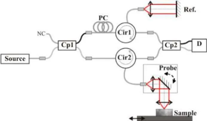
Technologies using a low-noise preamplifier. With these choices of swept source and sampling frequency, a depth range of 6.5 mm is available for the evaluation of the performance of the various methods. The actual setup is presented in Fig. 1.

Fig. 1. SS-OCT setup. Cp1 and Cp2: couplers, PC: polarization controller, Cir1 and Cir2: circulators and D: balanced detection.

3.2. Comparison of the processing methods

The performance of each signal processing method is evaluated from the point-spread functions (PSFs) obtained with a mirror at various depth locations in the sample arm. The parameters of interest are the amplitude of a PSF, the noise level, and the computational time. The amplitude of the PSF is expected to decrease when the mirror is displaced away from the zero-point delay. This is caused by the limited coherence of the swept-laser source in SS-OCT. This behavior is referred to as roll-off or fall-off. All the methods considered in this paper provide similar roll-off. Thus, the important parameter for comparing the methods is the amplitude of the PSF relative to the noise level. The quantitative determination of this noise level is somewhat arbitrary. It is not constant with depth and it is usually larger in the vicinity of the peak due to side lobes in the envelope function. We thus first compare PSF amplitude to noise level for the various methods from graphical representations of the PSFs. This allows observation of the additional spurious structures resulting from the application of some of the signal processing methods. We then evaluate signal-to-noise ratios for a more quantitative comparison. We finally look at the evolution of both the maximum amplitude of the PSF and the OCT resolution as a function of mirror position.

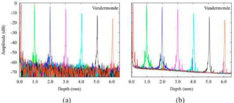
Averaging A-scans allows a better comparison of the signal processing methods. Figure 2(a) shows PSFs evaluated from a single A-scan for different mirror positions with the Vandermonde matrix method. A Hamming window is applied before processing the data. The noise for a single A-scan is fluctuating around a local mean value. These fluctuations are strong and do not allow a good evaluation of the PSF amplitude relative to the noise level. Our calculations show that the amplitude of the fluctuations is about 6 dB for all PSFs whatever the method used. Consequently, the fluctuations can be reduced by averaging to provide a mean noise level. This mean noise level then allows a better appreciation of the PSF amplitude relative to the noise level. This is illustrated in Fig. 2(b) where 1000 A-scans are averaged for each PSF evaluated at different mirror positions and processed with the Vandermonde matrix method. The noise level of all PSFs is clearly visible throughout the depth. One can always estimate the true noise for a single A-scan by adding a 6 dB fluctuation to the average noise of Fig. 2(b).

(10)

Fig. 2. PSFs after Vandermonde processing. (a) 1 scan per PSF. (b) averaging of 1000 A-scans per PSF.

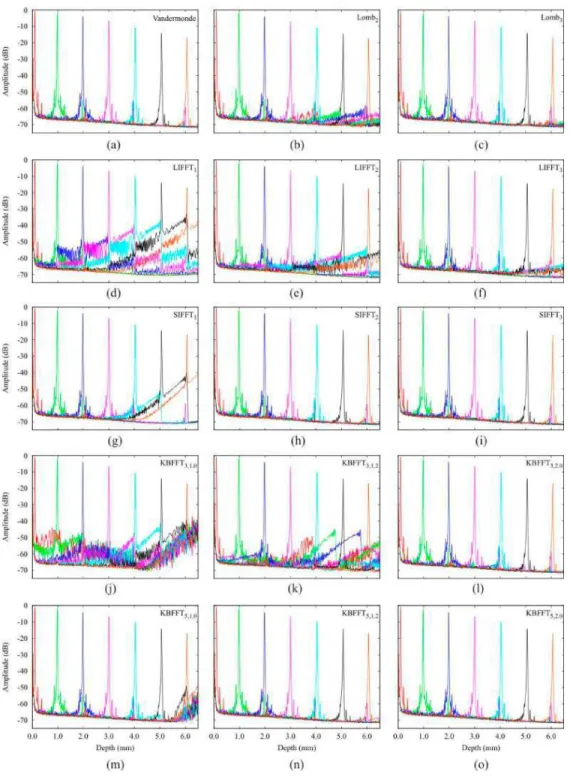
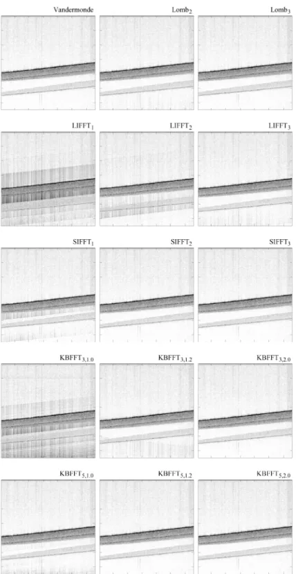
The PSFs evaluated with the various methods are presented in Fig. 3 while corresponding computational times are provided in Table 1. Each graph in Fig. 3 presents the PSFs evaluated for mirror positions from 0.1 to 6 mm, the 0 mm position being the zero-delay position of the sample arm. The different rows in Fig. 3 correspond to different signal processing methods. In all methods, a Hamming window is used to reduce leakage. For each row but the first one, the oversampling factor α used in a given method increases from left to right. Table 1 is organized similarly to Fig. 3 and provides the corresponding computational times for 1000 A-scans. Each A-scan is composed of N=1666 points. In the methods were a FFT is used, as mentioned in section 2, we use FFTPack which can be performed with a total number of points that is a product of small prime numbers. Accordingly, FFT are performed on resampled data zero-padded to 1672 points, 3332 points, and 5000 points, for oversampling factors of 1, 2, and 3, respectively. Apart from the Vandermonde matrix method, the computational times of the various methods are provided for optimized algorithms as discussed in Section 2, but running on a single processor. Further optimization could be obtained from multithreading for parallel computing as done in [35]. Also, reported computational times in recent work of FD-OCT show a wide range of performance, from 3000 ms down to 15 ms for 1000 A-scans, compared to our 200 ms computational time for the case of linear interpolation with an oversampling factor α=3 and FFT [15, 34–36]. The factor of about 200 between the different performances is uncertain and cannot be attributable only to the use of a few processors or of a more optimized FFT algorithm [42]. Comparing computational times from different publications thus appears to be a hazardous task. Consequently, the computational times of Table 1 should mainly be used to compare the relative efficiency of the various methods. All these computational times would decrease proportionally if multithreading was used.

The PSFs evaluated with non-uniform DFT methods are presented in the first row of Fig. 3. Figure 3(a) is obtained with the Vandermonde matrix method, considered as the reference.

(11)

Fig. 3. PSFs for various signal processing methods.

Apart from the variation of the PSF amplitude with the mirror position due to the roll-off, the PSFs are free from artifacts and the noise level for each PSF is low. The noise evolves quite similarly for all mirror positions and decreases with depth. As discussed in Section 2.1, the computational complexity of this method is larger than that of all other methods. Its good results come at a price in computational time. Table 1 indicates that processing 1000 A-scans takes over 3 sec. Our implementation of the Vandermonde matrix approach is not fully

(12)

optimized, but it is not expected that further optimization would reduce the computational time to that obtained with the other methods. The Lomb periodogram is a faster way for performing non-uniform DFT. Figure 3(b) presents the PSFs obtained with the Lomb2 method: the Lomb periodogram method with 2 Lagrange interpolation points (L=2). The computational time is much improved at 0.5 s for 1000 A-scans, but enlarged replicas appear 3 mm deeper than the main peak for all PSFs. This increases significantly the noise level. Using Lomb3 with 3 Lagrange interpolation points (L=3) as in Fig. 3(c) provides better PSFs with much smaller replicas. The computational time only slightly increases from the Lomb2 case. Consequently, the Lomb3 method is an efficient non-uniform DFT method, but it doesn’t compete in terms of computational time with the methods discussed below.

The PSFs in Figs. 3(d), 3(e), and 3(f) are obtained with linear-interpolation resampling followed by FFT with oversampling factors α = 1, 2 and 3, respectively. The method with its oversampling factor α is referred to as LIFFTα. LIFTT1 corresponds to no oversampling. Table 1 shows that the computational time for this case is the smallest of all methods considered in this paper with 80 ms for 1000 A-scans. For LIFFT2 and LIFFT3, the computational times increase to 137 ms and 199 ms, respectively. These computational times are much smaller than those for non-uniform DFT. For each PSF, Fig. 3(d) shows artifacts in the form of enlarged replicas that are spaced by approximately 1 mm. The amplitude of the replicas decreases away from the main peak of the PSF. In Fig. 3(e), these replicas are weaker and spaced by 2 mm. In Fig. 3(f), the replicas are even weaker and spaced by about 3 mm. Thus the spacing between the replicas scales with the oversampling factor and their amplitude decreases when the oversampling factor increases. These replicas are related to the error performed with the linear interpolation and to the nonlinearity of the swept-laser source. A swept-source with a different nonlinearity would lead to different pattern and periodicity. For the swept-source used in this work, these results indicate that LIFFTα provides acceptable

results only for an oversampling factor α larger than 3.

The PSFs in Figs. 3(g), 3(h), and 3(i) are obtained with a cubic spline-interpolation resampling followed by FFT with oversampling factors α = 1, 2 and 3. We refer to this method as SIFFTα. SIFFTα provides a much better signal-to-noise ratio (SNR) than LIFFTα with the same oversampling factor. There are fewer replicas and the noise level is much lower. Table 1 shows that the computational times are much larger at 230 ms, 328 ms, and 428 ms for the oversampling factors 1, 2, and 3, respectively. SIFFTα is extensively used in the OCT literature, although the level of oversampling is not always clearly specified. Figure 3(h) shows that SIFFT2 provides PSFs that are very close to those obtained with the Vandermonde matrix method in Fig. 3(a). SIFFT2 is nevertheless not optimal due to its rather large computational time.

The last two rows of Fig. 3 present the PSFs obtained with the convolution method using a Kaiser-Bessel window followed by FFT. Cases are identified by the maximum number of points used in the convolution (M=3 and 5) and the oversampling factor (α = 1, 1.2 and 2). They are referred to as KBFFTM,α. The parameter of the Kaiser-Bessel kernel takes the optimized value from Eq. (15). Figures 3(j) and 3(k) show that this method leads to enlarged replicas away from the main peak of each PSF for KBFFT3,1 and KBFFT3,1.2. These replicas are not present for KBFFT3,2 in Fig. 3(l). The results of KBFFT3,2 are very similar to those of SIFFT2, but with a computational time for 1000 A-scans 1.7 times smaller at 193 ms. Thus KBFFT3,α performs better than LIFFT3 and SIFFT2. Further improvement in computational time can be obtained by using more points in the convolution process. Figures 3(m), 3(n) and 3(o) presents PSFs obtained from KBFFT5,1, KBFFT5,1.2, KBFFT5,2, respectively. The corresponding computational times for KBFFT5,α in Table 1 are essentially the same as those for the KBFFT3,α cases with similar oversampling factors α. An important result is that replica-free PSFs with low noise levels are obtained with a smaller oversampling factor. With an oversampling factor of 1.2, the number of required points for the FFT, using FFTPack, is only 2000 points. This is a net gain when compared to any method requiring an oversampling factor of 2 where 3332 points are required. The results for KBFFT5,1.2 in Fig. 3(n) is very

(13)

similar to those of SIFFT2 in Fig. 3(h), but with a further reduced computational time more than 2.5 times smaller at 129 ms.

Table 1. Computational timesa_{for 1000 A-scans (ms).}

Method α or L 1 2 3 Vandermonde 3052 LombL 498 571 LIFFTα 80 137 199 SIFFTα 230 328 428 1 1.2 2 KBFFT3,α 112 129 193 KBFFT5,α 117 129 199

a_{Evaluated on a PC with an Intel Core2 Duo CPU T7700 @ 2.4 GHz and 3.5 GB RAM and running of one} processor.

Focusing solely on the SNR, Fig. 4 shows the evolution of the SNR as a function of depth for the different processing methods. The SNR is defined in this work as:

10 20 log 2 A µ SNR        _ _   (17)

where A is the maximum amplitude of a PSF, µ is the average noise level, and σ is the standard deviation of the noise. The parameters µ et σ are evaluated over a 200 µm region beginning 400 µm to the right of the main peak of the PSF. For a given method and depth, such SNR values are averaged over 100 A-scans. This definition provides a good criterion to assess how a PSF is affected by the noise far from its main peak.

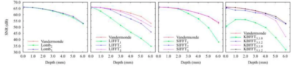
Fig. 4. SNR as a function of depth for different processing methods. For clarity, the results for the various methods are distributed over multiple figures, with the Vandermonde result being present in all the figures for reference.

Evolution of the SNR allows a more quantitative comparison of the various methods. The methods that provide a SNR similar to the Vandermonde method are: LombL for L  2, SIFFTα for α  2, KBFFT3,α for α  2, and KBFFT5,α for α  1.2. This confirms the previous observations made from the PSFs of Fig. 3.

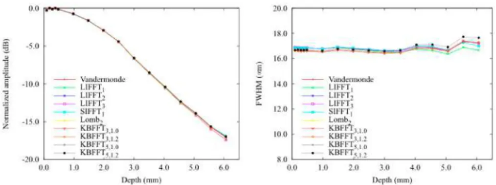
Finally, Fig. 5 shows the evolution of both the maximum amplitude of the PSF and the OCT resolution as a function of mirror position. The maximum amplitude of the PSF is the same for all the methods. This is why we noted at the beginning of this section that all the methods provided the same roll-off. Consequently, the variations in SNR observed in Fig. 4 between the different methods can be solely attributed to variations in noise level. The OCT resolution is evaluated from the full width at half-maximum (FWHM) of a PSF. Figure 5 shows that all methods provide the same OCT resolution. The OCT resolution is a bit enlarged to more than 16 μm due to the Hamming window applied to the data. Without a Hamming window, the measured OCT resolution is 12 μm but with larger side lobes in the envelope function.

(14)

Fig. 5. Maximum amplitude of the PSF (left) and FWHM (right) as a function of depth for different processing methods, after averaging over 100 A-scans.

The results of Figs. 3 to 5 and computational times in Table 1 indicate that KBFFT5,1.2 is the most efficient method. The convolution method in combination with a small fractional oversampling factor provides a very precise result without strongly impacting the computational time. This method produces results comparable to those of the Vandermonde matrix method in terms of PSF amplitude and noise level. It performs much faster than the often used SIFFTα no matter which oversampling factor is used in the latter.

3.3. Phantom and tissue imaging

The performance of the various signal processing methods is further evaluated from real OCT images of a multilayer phantom and of a finger nail. In both cases, a Hamming window is applied before processing the A-scans.

The multilayer phantom is made of 3 silicon layers with different concentrations of alumina powder. The scattering varies from one layer to another, so does the amplitude of the OCT signal. These phantoms are molded in a plastic cup. They are not removed from the cup for measurement and the bottom of the cup provides a 4th layer. The phantom fabrication process is a simplified version of the technology described in Bisaillon et al. [45] This artificial structure provides well-defined homogeneous regions and it is an ideal tool to evaluate the efficiency of a signal processing method.

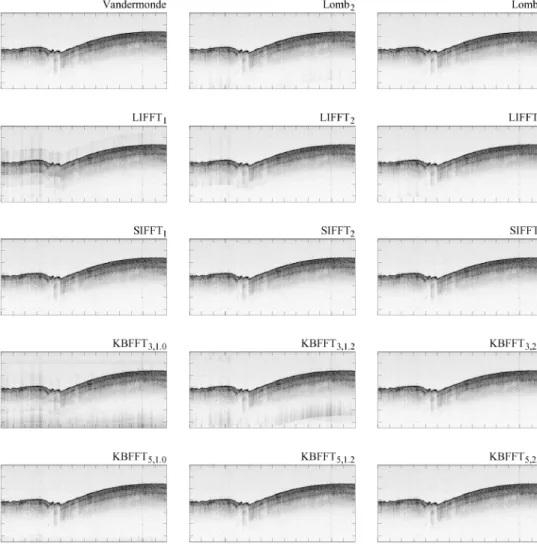
The OCT images obtained with the various methods are presented in Fig. 6 using an inverted gray scale. The arrangement in Fig. 6 is the same as that of Fig. 3 with each row corresponding to different methods. The reference image is the one obtained with the Vandermonde matrix method where the four layers are clearly delineated. The phantom is measured from the bottom and the uppermost layer thus belongs to the plastic cup. It provides an OCT amplitude similar to that of the subsequent phantom layer, but the two are separated by a dark line resulting from the strong reflection at the interface between the phantom and the cup. Many of the OCT images obtained with the different methods show ghost artifacts that can be related to the replicas observed in the PSFs of Fig. 3. Also in many images, the noise level is rather large, as it can be qualitatively estimated by looking at the difference in amplitude of the lowest phantom layer and of the empty region below. LIFFT3 provides a good image, although the noise level is still high. Very good results are obtained for SIFFT2, SIFFT3, KBFFT3,2, KBFFT5,1.2, and KBFFT5,2. This is in agreement with the analysis of the PSFs in Section 3.2.

(15)

Fig. 6. OCT images of a 4-layer phantom using different signal processing methods. Images are 6.5 cm wide by 6.5 cm deep. Each axis tic mark corresponds to 1 mm. Gray-scale is a log. scale, the dynamic range is 40 dB.

(16)

These results are further confirmed in Fig. 7 where OCT images of a finger nail are presented for the various signal processing methods. The arrangement of Fig. 7 is again the same as that of Fig. 3. Ghost artifacts are again present in many images. Best OCT images, similar to that of the Vandermonde matrix method, are obtained for SIFFT2, SIFFT3, KBFFT3,2, KBFFT5,1.2, and KBFFT5,2.

Amongst the methods that provide the best images for the phantom and the finger nail, Table 1 shows that KBFFT5,1.2 is the one with the smallest computational time. Thus KBFFT5,1.2 is the most efficient method providing the best trade-off between image quality and computational time.

Fig. 7. OCT images of a finger nail of a healthy volunteer using different signal processing methods. Images are 14.0 cm wide by 6.5 cm deep. Each axis tic mark corresponds to 1 mm. Gray-scale is a log. scale, the dynamic range is 40 dB.

4. Conclusion

A comparison of various methods to process the data in SS-OCT was performed by evaluating PSFs and by imaging a structured phantom and a finger nail. These methods include non-uniform discrete Fourier transforms with Vandermonde matrix or with Lomb periodogram, resampling with linear interpolation or spline interpolation prior to FFT, and resampling through convolution with a Kaiser-Bessel function followed by FFT. The non-uniform discrete Fourier transform methods provide very good results, but at a hard cost in

(17)

computational time. The methods involving linear or spline resampling were shown to perform rather poorly in terms of SNR or computational time. We introduced a new approach for SS-OCT signal processing based on an optimized version of the convolution method in which the Kaiser-Bessel window parameter is carefully selected to allow a minimal oversampling factor between 1 and 2. One can thus benefit from an efficient resampling technique while retaining small data structures. This method with a small fractional oversampling factor of 1.2 was shown to provide results similar to the method using spline interpolation with an oversampling factor of 2, but with a computational time 2.5 times smaller. Resampling through convolution using an optimized Kaiser-Bessel function with a small fractional oversampling factor should be considered as one of the methods of choice to obtain high quality OCT images in a small computational time. This conclusion also applies to spectral-domain OCT since the methods to correct for the non-linearity in wavenumber space resulting from spectrometers are similar to those used is SS-OCT.

Acknowledgements

This research was supported by the Genomics and Health Initiative of the National Research Council Canada. The authors gratefully thank Sherif S. Sherif for helpful discussions about the Vandermonde matrix method.