Bayesian inference of stochastic dynamical models

Bayesian Inference of

Stochastic Dynamical Models

by

Peter Lu

Submitted to the Department of Mechanical Engineering

in partial fulfillment of the requirements for the degree of

Master of Science in Mechanical Engineering

at the

MASSACHUSETTS INSTITUTE OF TECHNOLOGY

February 2013

©

Massachusetts Institute of Technology 2013. All rights reserved.

A u th o r ...

Department of Mechanical Engineering

January 18, 2013

Certified by

Pierre F.J. Lermusiaux

ssociate Professor of Mechanical Engineering

Thesis Supervisor

A ccepted by ...

...

David E. Hardt

Chairnan, Departiment Conmuittee on Graduate Theses

Bayesian Inference of

Stochastic Dynamical Models

by

Peter Lu

Submitted to the Department of Mechanical Engineering on January 18, 2013, in partial fulfillment of the

requirements for the degree of

Master of Science in Mechanical Engineering

Abstract

A new methodology for Bayesian inference of stochastic dynamical models is

devel-oped. The methodology leverages the dynamically orthogonal (DO) evolution equa-tions for reduced-dimension uncertainty evolution and the Gaussian mixture model

DO filtering algorithm for nonlinear reduced-dimension state variable inference to

perform parallelized computation of marginal likelihoods for multiple candidate mod-els, enabling efficient Bayesian update of model distributions. The methodology also employs reduced-dimension state augmentation to accommodate models featuring un-certain parameters. The methodology is applied successfully to two high-dimensional, nonlinear simulated fluid and ocean systems. Successful joint inference of an uncer-tain spatial geometry, one unceruncer-tain model parameter, and 0(105) uncertain state variables is achieved for the first. Successful joint inference of an uncertain stochastic dynamical equation and 0(105) uncertain state variables is achieved for the second. Extensions to adaptive modeling and adaptive sampling are discussed.

Thesis Supervisor: Pierre F.J. Lermusiaux

Acknowledgments

Thank you to my advisor and colleagues. Thank you to my friends and family.

Contents

1 Introduction 11

1.1 Stochastic Dynamical Systems . . . . 11

1.2 Model Formulation Uncertainty . . . . 12

1.3 Literature Review . . . . 14 1.4 Problem Statement . . . . 16 1.4.1 System . . . . 16 1.4.2 Observations . . . . 17 1.4.3 G oal . . . . 18 1.5 Candidate Models . . . . 18

1.6 Bayesian Model Inference . . . . 20

1.7 Overview of the Present Work . . . . 22

2 Marginal Likelihood Calculation 25 2.1 Overview . . . . 25 2.2 Analytical Cases . . . . 25 2.3 Asymptotic Approximations . . . . 27 2.4 Computational Approximations . . . . 28 2.5 Summary . . . . 31 3 Methodology 33 3.1 Overview. . . . .. . . . . 33 3.2 DO Evolution Equations . . . . 36 3.3 GMM-DO Filter . . . .. . . . . 40

3.4 Reduced-Dimension State Augmentation . .

3.5 GMM-DO Marginal Likelihood Calculation.

3.5.1 Analytical GMM Approach . . . . .

3.5.2 Computational Alternatives . . . . .

3.6 Summary . . . .

3.6.1 Comments . . . .

4 Flow Past an Obstacle

4.1 Flow Past a Cylinder or Island . . . . 4.2 Stochastic Flow Past an Obstacle System . . . . 4.3 Description of the Experiments . . . . 4.3.1 Model Formulation . . . . 4.3.2 True Solution Generation . . . .

4.3.3 Observations and Inference . . . . 4.3.4 Numerical Method . . . . 4.4 R esults . . . . 4.4.1 Experiment Al: Circular Obstacle . . . . 4.4.2 Experiment A2: Downstream-Pointing Triangular Obstacle

5 Microorganism Tracer

5.1 Marine Microorganisms . . . .

5.2 Stochastic Microorganism Tracer System . . . .

5.3 Description of the Experiments . . . .

5.3.1 Model Formulation . . . .

5.3.2 True Solution Generation . . . . 5.3.3 Observations and Inference . . . . 5.3.4 Numerical Method . . . . 5.4 R esults . . . . 5.4.1 Experiment B1: Constant Growth and Decay 5.4.2 Experiment B2: Constant Growth and

Spatially-Variable Decay . . . . 97 . . . . 97 . . . . 98 . . . . 103 . . . . 103 . . . . 105 . . . . 107 . . . . 107 . . . . 108 . . . . 109 . . . . 118 . . . . 45 . . . . 49 . . . . 49 . . . . 51 . . . . 53 . . . . 56 59 59 63 64 64 70 71 72 73 74 89

5.4.3 Experiment B3: Time-Dependent Growth and

Spatially-Variable Decay . . . . 124 5.4.4 Experiment B4: Intermediate Time-Dependent Growth and

Spatially-Variable Decay . . . . 130

6 Discussion 139

6.1 Adaptive M odeling . . . . 139

6.2 Adaptive Sampling . . . . 141

6.3 Conclusion . . . . 143

A Convolution of Gaussian Distributions 145

B Derivation of the DO Evolution Equations 149

C Subspace Equivalency in the GMM-DO Filter 155

D Microorganism Reaction Equation Linearization 161

Chapter 1

Introduction

1.1

Stochastic Dynamical Systems

A stochastic dynamical system is any system that is both

time-varying--dynamical-and affected by uncertainty-stochastic [59]. Examples of such systems are every-where. Physical systems such as oceans and ecological networks, engineering systems such as power grids and communications networks, and anthropological systems such as financial markets and social networks can all be classified as stochastic dynamical systems. The mathematical tools that have been developed for investigating stochas-tic dynamical systems are thus highly versatile and have been applied in a wide range

of fields [4, 5, 12, 25, 36, 51, 62, 66, 87, 116, 117, 118].

The general procedure for modeling a stochastic dynamical system is best illus-trated with a simple example: a ball thrown through the air. This system is certainly dynamical; the ball's position and velocity, the state variables of the system, are changing with time. The system is also stochastic; the ball's trajectory is depen-dent on its initial conditions, which can be uncertain, as well as on turbulent mul-tiscale aerodynamic forcings, which are often not deterministically predictable. The evolution of the ball's position and velocity can be mathematically described by a stochastic differential equation (SDE) that couples Newton's laws of motion with sta-tistical representations of the turbulent aerodynamic forcings. This SDE represents the stochastic dynamical model for the system. Given a probability distribution for

the ball's initial conditions, the stochastic dynamical model can be used to predict probability distributions for the ball's position and velocity as functions of time, a process known as predicting the uncertainty evolution. If observations of the ball are made during the course of its flight, these probability distributions can be updated to account for the newly-acquired information, a process known as inference or data assimilation. Inference always reduces uncertainty in a system's state variables.

The general procedure for modeling a stochastic dynamical system can be sum-marized as follows:

1. Model formulation. Formulate a stochastic dynamical model that governs the

evolution of the system's state variables and their associated probability distri-bution.

2. Uncertainty initialization. Quantify initial uncertainty in the system's state variables by specifying an initial probability distribution.

3. Uncertainty evolution. Evolve the initial state variable probability distribution

through time using the stochastic dynamical model.

4. Inference. Update the state variable probability distribution using information from observations, reducing state variable uncertainty.

Though listed sequentially, uncertainty evolution and inference typically occur in an alternating fashion, with periods of uncertainty evolution interspersed with instances of inference. We also note that uncertainty evolution and inference can also be com-pleted backward in time.

1.2

Model Formulation Uncertainty

For the example featuring the ballistic ball, it was implicitly assumed that the stochas-tic dynamical model formulated for the system was an accurate mathemastochas-tical descrip-tion of its governing physics. Uncertainty in the system's state variables was modeled

as originating solely from uncertainty in the system's initial conditions and the tur-bulent aerodynamic forcings, whose statistical properties were assumed known. This assumption of absolute validity of the model formulation however is not always defen-sible. For the ball, Newton's laws of motion were included in the system's stochastic dynamical model, but what if these laws were uncertain? That is, what if the ball were being thrown during a pre-Newtonian era when it was not known whether force was proportional to velocity, acceleration, or a non-linear function of both? This source of uncertainty-model formulation uncertainty-would certainly amplify the overall uncertainty in the ball's trajectory. In contemporary contexts, similar model uncertainty could arise when dealing with complex systems whose governing equa-tions have not yet been derived from known first principles. For these systems, the assumption of absolute validity for any one particular model formulation would surely be inappropriate. In general, uncertainty in model formulation can originate from the choice of state variables themselves, from the functional forms of the model equations, the boundary conditions, and initial conditions, and from the definition of the (spa-tial) domain of integration. Both the deterministic and stochastic components of the model formulation can be uncertain. In what follows, when possible, we will we refer to model formulation uncertainty as simply model uncertainty.

Model uncertainty in stochastic dynamical systems can be difficult to properly quantify and is thus often ignored. This simplifying assumption is not severely dam-aging when model uncertainty is insignificant. When throwing a ball on Earth in the

2 1st century for example, one can have high confidence in the validity of Newton's laws

of motion. In other cases however, it can lead to significant underestimation of state variable uncertainty. [34], [55], and [72] review poignant examples from the statistics literature in which ignorance of model uncertainty resulted in overconfidence in state variable estimates, which subsequently led to tragically flawed conclusions.

Perhaps even more unfortunate, ignoring model uncertainty is antithetic to the scientific method, which entails the comparison of competing hypotheses by means of observations. If multiple models are considered, the same observations of a stochastic dynamical system that are used to perform inference of its state variables can also

be used to infer the relative validity of each of the models. This process of model inference can reveal valuable insights regarding the fundamental mechanisms that govern the system under investigation. If model uncertainty is ignored however and only one model-one hypothesis-is assumed, this opportunity for scientific discovery in the classic sense is forfeited.

1.3

Literature Review

Several methods have been developed to handle the coupled issues of model uncer-tainty and model inference in stochastic dynamical systems. We review a number of these methods here.

Directed search methods are a general class of computational methods for model inference. These methods typically proceed by first performing state variable inference for a large set of candidate models, then scoring the inferred state variables relative to system observations using metrics derived from frequentist statistics. Computa-tional schemes are employed to search through expansive sets of plausible candidate models, with the search process directed by results from successive rounds of can-didate evaluations. [123] is a premier example of this strategy. In this work, the authors employed a heuristic optimization scheme known as symbolic regression [75] to search through a space of algebraic expressions with the goal of finding the fun-damental physical laws that govern several simple dynamical systems, such as single and double pendula. The authors were able to identify conservation laws for en-ergy and momentum without any prior information regarding the laws' functional forms. Their approach was highly versatile but exceptionally demanding in terms of computational cost, even for the low-dimensional systems considered in their work. Model inference for the double pendulum system, a non-linear system with two state variables, required over 30 hours of computational time in a 32-core parallelized imple-mentation. Extensions of their approach, and other directed search model inference methods (e.g. [19, 22, 74, 110, 144]), to high-dimensional systems will likely prove to be computationally challenging.

Hierarchical Bayesian modeling is a general approach to handling model uncer-tainty whereby full stochastic dynamical models are represented as hierarchies of sim-pler, analytically tractable sub-models [145, 147]. If these sub-models are properly formulated, inference can be performed separately for each by exploiting their con-ditional independences, with the sub-models aggregated afterwards to achieve global model inference. An oceanographic application of this approach is demonstrated in [146], where the authors used a hierarchical Bayesian model to formulate a stochastic dynamical model of the surface wind streamfunction over a region of the Labrador Sea using satellite surface wind velocity data. The aggregate wind model was decom-posed into sub-models for observational data, boundary conditions, and the numerical streamfunction, which enabled the quantification of boundary condition uncertainties on the posterior distribution of streamfunction values. [60] features an ecological ap-plication of this approach, where the authors used a hierarchical Bayesian model to predict the spatial distribution of ground flora based on sparse data. Sub-models were formulated that enabled the incorporation of geographic covariates, a source of model uncertainty that, when accounted for, significantly enhanced flora distribution predictions. [16], [61], [103], [114], and [131] present further applications of hierar-chical Bayesian modeling to problems of spatiotemporal statistics. Multiresolution Bayesian modeling, a variation of the approach for application to signal and image processing, is reviewed in [27], [28], and [148]. [65] reviews an extension of the hierar-chical formulation to graphical models that allow for more complex interdependencies between model components at the cost of more computationally intensive inference algorithms.

Reduced-order modeling is a set of methods that have been employed to deal with high-dimensional systems featuring model uncertainty [40]. Though many model inference techniques, such as the directed search methods reviewed above, can be effective when system dimensions are small and candidate model spaces are readily explored, computational difficulties often arise when the same techniques are applied to high-dimensional systems, such as those frequently encountered in oceanography

repre-sentations of high-dimensional models, for which model uncertainty quantification and inference are more readily performed. A wide selection of methods fall under this clas-sification, including proper orthogonal decomposition [7, 20, 53], centroidal Voronoi tessellation [23], neural networks [44, 142], Volterra series [99], kriging [49], certified reduced basis methods based on numerical error bounds [64], empirical emulators

[97, 134], error subspace statistical estimation (ESSE) [83, 90],and the dynamically

orthogonal (DO) evolution equations [120, 121]. Though these techniques all take advantage of information redundancies in full-order stochastic dynamical models to achieve order reduction, some (e.g. the DO evolution equations) preserve decidedly greater physical meaning in their low-dimensional representations than others (e.g. neural networks and empirical emulators).

The methodology developed in the present work adopts ideas from both hier-archical Bayesian modeling and reduced-order modeling to achieve efficient model uncertainty quantification and inference for stochastic dynamical systems of large di-mension. Other works directly relevant to the present methodology are reviewed later in Chapters 1 and 2.

1.4

Problem Statement

1.4.1

System

In this work, we consider a general stochastic dynamical system with state vector

X (E RNx governed by an uncertain stochastic dynamical model M with uncertain

parameter vector E E RNe, where Nx E N and N9 E N are the dimensions of the state and parameter vectors respectively. For realizations x, 0, and M, of X,

E,

and M respectively, we have

dx(t; w) = M _{[ x(t; W), 0(w), t; W]}

(1.1)

dt

where t denotes time, w an index over stochastic realizations (a random event), D. the set of stochastic dynamical equations for the model, SG, the spatial geometry (spatial domain), BC, the boundary conditions, and IC,, the initial conditions. All of the model components represented in (1.2) are allowed to be uncertain. The joint

probability distribution over

X,

E,

and M is defined to be px,e,M(x, , Mn).

1.4.2

Observations

Stochastic observations Y

C

RNY of the system's state variables are assumed to

be available at arbitrarily times, with the probability distribution of observations conditionally independent of both the stochastic dynamical model and the parameters given state variables

pyIx,e,M(yIx,O,Mn) = pyIx(yIX) =f(ylX) VX

e

N

(1.3)

where Ny E N is the dimension of the observation vector, y represents a realization of the observation vector, and L(y Ie) represents the observation likelihood function or observation model for the system.

One particular observation likelihood function we will use is a Gaussian distribu-tion, for which we have

L(ylx)=N(y; Hx, R) Vx E RNx (1.4)

where A(.e; p., E

)

represents a multivariate Gaussian distribution with mean yt and

covariance E, H E RNYxNx represents the linear observation matrix that transforms

state variables into observation means, and R E RNYxNy represents the matrix of

ob-servation covariances. This particular obob-servation model is equivalent to the following linear relation between state and observation vectors:

Y=HX+V,

obser-vation model is assumed to be time-invariant (i.e. the parameters H and R in the particular case of (1.4) are assumed to be time-invariant).

1.4.3

Goal

The goal of the present work is two-part:

1. Efficiently evolve px,e,M(x, 0, M,) in time, accounting for all forms of

uncer-tainty encapsulated in (1.1) and (1.2).

2. When observations are available, perform the update

px,e,M (x, , Mn) -+ Px,e,MI Y(X, , MnIy)

using the observation model represented by (1.3).

1.5

Candidate Models

When faced with a stochastic dynamical system whose model is uncertain, a common approach is to formulate a finite set of candidates for the true model governing the system under investigation. These candidate models or beliefs may be derived from first principles, may be inspired by previous observations, or may be based on a combination of theoretical and empirical prior knowledge. A discrete probability distribution pM(e) can be defined over the set of candidate models to represent the probabilities that each of the candidates are the true model. We note that in general the candidates can be correlated. In a Monte-Carlo approach, each candidate model can be used to predict the evolution of the uncertainties of the system's state variables independent of the other models, producing state variable probability distributions that are conditional on the candidates being the true model.

If the candidate models are assumed to be independent, a state variable

probabil-ity distribution that accounts for the uncertainty in the formulation of the system's stochastic dynamical model can be estimated at any time as simply the weighted

average of these conditional distributions

NM

px(x) = ZpxiM(x|M.)pM(M.) Vx E RNX (1.5) n=1

where px(o) represents the state variable distribution, NM E N represents the

total number of candidate models, Mn represents the nth candidate model, and PxI M (0 1 Mn) represents the state variable distribution conditioned on the nth can-didate model (the nth model-conditional state variable distribution). This general approach to accounting for model uncertainty has been used in many fields and is known by many names, including Bayesian model averaging [55, 112, 126], multimodel estimation [11, 101], multimodel fusion [98], and (multimodel or super-) ensemble modeling [50, 76, 115]. We note that if the candidate models Mn are correlated or if the space of model formulation/structures is continuous (instead of discrete as in

(1.5)), the distribution (1.5) becomes a correlated weighting or an integral over the

continuous model formulation/structures. Our formalism can be extended to these cases and this will be reported elsewhere.

In the present case, the linear nature of (1.5) w.r.t. candidate models leads to several useful properties. Marginal distributions for subsets of state variables can be found as weighted averages of the corresponding model-conditional marginal distri-butions. Letting x1 and X2 be mutually exclusive complementary subsets of state

variables and x =

[X

1 X2]T, Px 1(xi) px(x) dX2 PX(I X1 X 2 ]T2) dX2 Nm E PX|M X1 X2 ]TMn d ₂ )PM (Mn) NM = j PX1|M(X1 IMn)PM(Mn) Vxi E RNx, (1.6)

where Nx, < Nx. Similarly, the state variable mean can be found as a weighted average of the model-conditional state variable means

E[X] JXPx(x) dx X Nm = Jx ( pxM(x|Mfl)pM(M) dx n=1 - XPXIM(xIMn) dx) PM(Mn) Nm -E [XM n1PM(Mn) (1.7) n=1

1.6

Bayesian Model Inference

When observations of a stochastic dynamical system's state variables are made, both the model-conditional state variable distributions and model distribution within the

summation of (1.5) can theoretically be updated using Bayes' theorem [13]

PXIY,M(XIY,MAn) = PYIM(Y

IXM)

pXIM(XI.An)

Vx E RNx,Vn E{l,..., NM}, (1.8)

PYIM(y|Mn)

PMY(MAn

IY)

=

(

)

PM(Mn) Vn E {1,..., NM}. (1.9) py(y)

In (1.8), the model Mn plays the role of a 'given parameter'. For this Mn, the distributions pxIM(e|lM) and pxY,M(e

l

y, Mn) are referred to as the prior and posterior conditional state variable distributions for the nth candidate model respec-tively, while pM(e) and pMI y(o

I

y) are referred to as the prior and posterior model

distributions.

If the candidate models are assumed independent, as in (1.5), the posterior

form the posterior state variable distribution

NM

pxiy(xy) = ZpXiy,M(xjy,M)pMiy(Mn|y) Vx E RNx (1.10)

(1.8) represents Bayesian state variable inference and can be performed for each

model-conditional state variable distribution independently, ignoring model uncer-tainty. Techniques for state variable inference abound, ranging from classic ana-lytical methods such as the Kalman filter [69, 70] to contemporary computational approaches such as particle filters [6], Markov chain Monte Carlo (MCMC) algo-rithms [3], and forward-backward algoalgo-rithms [37]. State variable inference and data assimilation have roots in optimal estimation theory e.g. [45, 68, 124] and control the-ory [95, 82], with now many applications in environmental sciences and engineering

(e.g. [15, 71, 79, 100, 111, 117, 145, 149]).

(1.9) represents Bayesian model inference. The comparison of the posteriors for

each M., pMIy(M, y), is Bayesian hypothesis testing for competing models and each pMIy(M, y) is often referred to as model evidence. Though cosmetically

sim-pler than (1.8), (1.9) is in fact the more challenging of the two Bayesian updates to perform. The chief difficulty lies in the calculation of the marginal likelihood

p i m (y

I

M.), which represents the strength of the observational evidence for the nth candidate model, i.e. the likelihood of model M,, for all states X. While

PYiXM (y

I

x, M,) is equivalent to the observation likelihood function L(y

I

x)-the function that defines the probability distribution for observations when state variables are known-an explicit expression for the likelihood pri M (y

I

M.) is not available. Instead, PYJ M (y

I

M,) (the probability distribution for the observation vector real-ization conditioned on a given candidate model) must be found through oftentimes

difficult (large-dimension) integrations [34, 145, 138]

PYIM(YIMn) = jPYix, M(YzxM.)PxiM(XIMn) dx

Note that although pyiM(y|M.) also appears in (1.8), there it serves only as the normalization constant for the posterior conditional state variable distribution and its explicit calculation is usually side-stepped by Bayesian state variable inference schemes. Likewise, py(y) appearing in (1.9) is not of concern for inference, as it serves only as the normalization constant for the posterior model distribution. Once all marginal likelihoods have been found, py(y) can be computed as simply their weighted summation

NM

py(y) = PYM(Y|Mn)PM(Mn). (1.12)

n11

It is not uncommon that the difficulty of computing the integral in (1.11) leads to the avoidance of the update of the model distribution (1.9) entirely [76, 112]. In these cases, prior statistical knowledge derived from a fixed set of system observa-tions is typically used to specify an initial model distribution, which is then kept unchanged even when new observations become available. This approach is subop-timal, as update of the model distribution yields two significant benefits: 1) More precise weighting of the conditional state variable distributions in (1.5), leading to improved state variable uncertainty quantification (1.10); and 2) Insight into the true model governing the system under investigation. Techniques for the efficient compu-tation of the marginal likelihood integral in (1.11) are thus of great utility for the study of stochastic dynamical systems featuring uncertainty in model formulation.

1.7

Overview of the Present Work

The present work develops a new methodology for performing Bayesian inference of stochastic dynamical models. The dynamically orthogonal (DO) evolution equations for reduced-dimension uncertainty evolution [121] and the Gaussian mixture model

DO filtering algorithm (GMM-DO filter) for nonlinear reduced-dimension inference

of state variables [129, 130] are first extended to accommodate stochastic dynamical models featuring uncertain parameters. Another extension then enables the

compu-tationally expedient calculation of the marginal likelihood integral in (1.11). The result is a methodology capable of performing Bayesian model inference for high-dimensional, nonlinear stochastic dynamical systems, including oceanic and atmo-spheric systems.

Chapter 2 reviews a number of techniques that have been developed to calculate the marginal likelihood integral in (1.11), with particular attention paid to the added difficulties that arise with high-dimensional systems. Chapter 3 reviews the DO evolution equations and the GMM-DO filter, then develops the extensions of the new methodology in detail. Chapter 4 applies the methodology to a simulated stochastic dynamical system featuring a fluid flowing past an obstacle; model uncertainty arises in the shape of the obstacle. Chapter 5 applies the methodology to a second simulated system featuring a marine microorganism convected by a fluid; model uncertainty arises in the reaction equation of the microorganism. Chapter 6 provides a synopsis and a discussion of promising avenues for future investigation.

Chapter 2

Marginal Likelihood Calculation

2.1

Overview

As introduced in Chapter 1, the key computational difficulty associated with Bayesian model inference for a set of model candidates is the calculation of the marginal like-lihood integral

pyIM(yIM.) =

I

C(yjx)pxIm(xjM.) dx. (2.1)

Three classes of methods for performing this crucial calculation are reviewed in this chapter in order of increasing computational expense. The applicability of each of these method classes is dependent on the functional forms of the observation likelihood function L(y Ie) and model-conditional state variable distribution pxiM(*IMa). Note that (2.1) need not be calculated using the same method for all candidate mod-els. Indeed, the functional form of pxiM(e|Mn) for some candidates may enable computational expediencies not applicable to others.

2.2

Analytical Cases

In a handful of special cases, the functional forms of the observation likelihood func-tion L(y

Ie)

and conditional state variable distribution pxI m(e

I

M) allow for the

analytical calculation of the integral in (2.1).

One such case is when both L(y

I

e) and pxiM(e|IM) are Gaussian distributions.

Let

L(yIx)=(y; Hx, R) Vx E RNx

as first defined in (1.4). Further, let

pxIM(x|Mfn) =A(x; t

XIMn, EXIMn)

Vx

E

RNx

where p'XIMn E RNx represents the vector of state variable means conditional on the

nth candidate model and EXiMn E RNxxNX represents the matrix of state variable

covariances conditional on the nth candidate model.

Then, (2.1) becomes

PYIM(YIMn) =

(y;

Hx, R)N(x; p'XIM EXIMn) dx. (2.2)

Since the integral in (2.2) is taken over all values of x, a linear transformation of the integration variable can be performed without changing the value of the integral. Then, using the linear transformation properties of Gaussian distributions, (2.2) can be rewritten as

PYIM(YIMn)= J

(y

- Hx; 0, R)Af(Hx; HiXIM., HEXIMnHT

)

dHx. (2.3) Observations are assumed to be unbiased. (2.3) represents the convolution of two Gaussian distributions and thus yields another Gaussian distribution whose mean and variance are equal to the sums of the means and variances of the two component distributions respectively [35]

pri(ylM-)=

Ni(;

0, R)*N(*; HyJXIM

, HExim,

H(T

(y)

where * represents the convolution operator, defined as

[f(s)* 9(e)]

(t) =

J

f(t

- r)g(T) dT .

The full derivation of the convolution identity used in (2.4) is provided in Appendix A. Even if the conditional state variable distribution p xi M (e I M.) is not Gaussian, (2.4) can still be used to analytically calculate an approximation of the marginal likelihood if the mean and covariance of the conditional distribution is used to form a Gaussian approximation of the distribution. In control theory, state estimation schemes that are based on the classic Kalman filter typically already employ such Gaussian approximations and the extension of these schemes to perform Bayesian model inference using (2.4) has thus been natural [11, 101]. Though these Gaus-sian approximation methods are computationally expedient, they are limited in the complexity of the systems they can accomodate. Most conspicuously, systems that feature substantially non-Gaussian state variable distributions are handled poorly. A remedy for this-Gaussian mixture model (GMM) approximations-will be explored in Chapter 3. High-dimensional systems also pose a challenge as the size of the condi-tional state variable covariance matrix appearing in (2.4) grows as Nx 2, the square of the number of state variables. More versatile techniques are reviewed in the following

sections.

2.3

Asymptotic Approximations

When the functional forms of L(y

Ie)

and pxIM(9 1M,) do not allow for the ana-lytical calculation of the integral in (2.1), a popular alternative is to use closed-form approximations of the integral that are exact in the limit of infinite observations [72]. The majority of these asymptotic approximations are variations of the Laplace ap-proximation. The general Laplace approximation for an integral of the form f ef(u) du is

ef(u) du ~ (27)d/2 IA*l/

where u is a vector, d is the dimension of u, u* is the maximizing argument of

f

(.),

and A* is the negative of the inverse Hessian of

f

(*) evaluated at u* [9]. Substituting

log [L(y Ix) pxIm (x|

M )]

for

f

(u) yields the Laplace approximation for (2.1)

pylM (y M.) (27r)Nx/2 IA*11 2L(y x*)px|M(x* Mn) , (2-6)

where

x*

is the maximizing argument of log

[

L(y

I

*) pxIM(0 1M )], which is

equiv-alently the maximizing argument of L(y

Il)

pxIM

I

Ma),

and A* is the negative

of the inverse Hessian of log

[L(y

0) PxIM(0 | Mn)] evaluated at

x*.

Depending on

the functional forms of L(y 1 e) and pxIM(e|Mn), it may not be possible to find x* and A* analytically, in which case sample approximations for x* and A* must be found before (2.6) can be evaluated, e.g. [92].

The accuracy of the Laplace approximation and its variants increases as the

den-sity of L(y

l

e)pxiM(e|IM) increases near its maximum (i.e. the more the density

peaks, the better). These asymptotic approximations are thus best-suited for systems featuring unimodal state variable distributions and large numbers of observations. Unfortunately, in high-dimensional, nonlinear systems such as those encountered in oceanography and meteorology, multimodality and sparse observations are the norm (e.g. [8, 31, 88, 87, 30, 100]). Furthermore, calculating and inverting the Hessian of

log [ L(y

I

e) pxim(9 | Mn)], which is necessary for (2.6), is computationally infeasible for systems of high-dimension and hence also needs to be approximated.

2.4

Computational Approximations

For cases where analytical solutions to (2.1) are not available and asymptotic approx-imations are inappropriate, computational approxapprox-imations are the only recourse. A general class of computational techniques known as importance sampling [33, 132] makes use of samples drawn from a chosen sampling distribution g(e) to approximate

(2.1) as the weighted average of numerous likelihood function evaluations

Ek_1 wk

L(yIXk)

(2.7)

P YIM(Y|Mn) K

Ek=1 Wk

where Xk represents the kth of K E N samples and the weights are defined by

Wk = PXIM(Xk|Mn) Vk

E

{1,... ,K}. (2.8)

9 (xk)

A sample weight is large when the density of the prior conditional state variable

distribution at the sample value is high relative to the density of the sampling dis-tribution g(e). The sample weights thus balance the frequency with which sample values are drawn from the sampling distribution and their 'importance' relative to the prior conditional state variable distribution.

The simplest choice for g(e) is the prior conditional state variable distribution itself, which reduces all sample weights to one and (2.7) to

priM (y1Mn) L(ylx) , (2.9)

k=1

where x represents the kth sample from the prior distribution. This is known as the arithmetic mean estimator (AME) [81]. Though the simplicity of its implementation is attractive, the AME can exhibit slow rates of convergence if L(y

I

e) is large for

only a small subset of its domain.

(2.7) becomes

K PXIM (Xk In)

PX|M y,

M

n k

k=1 P X |Y,M( k n)

pXIM(Xkj )

k-i PxY,M (4+IyMfl)

PXIM (Xk IMn)

k=1 PX|Y,M(kyMn)PYM(yIMn) )

K PX|M(xkIMn)

k1 PXYM(41YMn)PYIM(Y|Mn)

where x4 represents the kth sample from the posterior distribution. Using (1.8),

K ₁ PY|M(Y Mn)

L(ylx+)

1: 1 k=1 PYIXMY Xk, n) k-i pYI x,M (Y I Xk,Mn) K k=1 1

L (y Ix+)

L(yj4)

K L=(y1) K L Y k -L k=1

This is known as the harmonic mean estimator (HME) [108]. The convergence rate of the HME is typically faster than that of the AME due to the fact that the pos-terior conditional state variable distribution tends to have greater density than the prior distribution in areas where C(y I*) is large. This is a direct result of Bayesian state variable inference; the posterior distribution is generated by shifting the prior

distribution towards state variable values that are more likely to have produced the observations-i.e. values for which E(y

I *)

is large.

More advanced sampling techniques generally employ recursive schemes that ei-ther bias or constrain the sample distribution g(o) to regions where L(y 1 e) is large. These techniques include bridge sampling [102], path sampling [46], annealed impor-tance sampling [107], and nested sampling [29, 125]. Though the use of recursive adjustments to g(o) can greatly improve both convergence rate and stability, these advanced sampling techniques are still limited in the dimension of the systems they can handle. Even the best contemporary sampling techniques are limited to problems of dimension 0(102) [46], which falls far short of the 0(106-109) systems frequently encountered in the geophysical sciences [89]. At a fundamental level, sampling tech-niques are stymied by the fact that state space volumes grow as exponential functions of the number of the state variables. The number of samples needed to thoroughly can-vass a high-dimensional state space in order to accurately approximate the marginal likelihood integral in (2.1) is thus prohibitively large.

2.5

Summary

High system dimension is the common stumbling point of the marginal likelihood calculation methods reviewed in this chapter. In order to perform Bayesian model inference for high-dimensional stochastic dynamical systems, the major challenge is to derive inference schemes that can reduce the dimension of the systems down to a manageable order while capturing and exploiting dominant nonlinear dynamics and non-Gaussian statistics as they arise. Chapter 3 will show that the DO evolution equations are an effective means of achieving this dimension reduction. Further-more, Chapter 3 will also show that the GMM approximations employed by the GMM-DO filter allow for the analytical calculation of the marginal likelihood inte-gral in (2.1), while still providing the structural flexibility necessary to accommodate systems featuring nonlinear, multimodal state variable distributions. Together, the

Chapter 3

Methodology

3.1

Overview

To achieve the efficient dimension-reduction necessary for performing the marginal likelihood calculations (1.11) for high-dimensional stochastic dynamical systems, the present methodology employs the DO evolution equations to evolve the dominant model-conditional state variable distributions in (1.5). The GMM-DO filter is used to perform the Bayesian updates of the model-conditional distributions represented

by (1.8) in the evolving DO subspace. Reduced-dimension state augmentation is

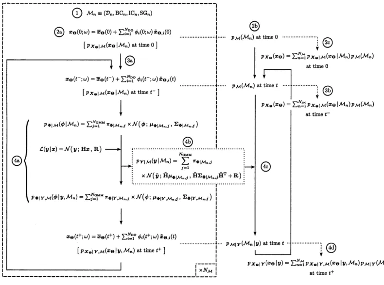
used to extend the DO evolution equations and the GMM-DO filter to accommodate stochastic dynamical models featuring uncertain parameters. The marginal likelihood calculations (1.11) are then performed analytically using Gaussian mixture models (GMM) in the DO subspaces for each candidate model, extending the Gaussian ap-proximation reviewed in Section 2.2. Finally, these marginal likelihoods are used to perform the Bayesian update (1.9) of the model distribution, thus accomplishing Bayesian model inference. Each of these components of the present methodology is developed in detail in the following sections, with an integrated account of the methodology provided at the end of the chapter. A compendium of the notation used in this chapter is provided in Table 3.1 for ease of reference.

Table 3.1: Notation compendium.

General

Nx E N dimension of state vector

X E RNx state vector

x E RNx state vector realization

Ne E N dimension of parameter vector

E

E RNe parameter vector

-0 E RNe parameter vector realization

M stochastic dynamical model

NM E N number of candidate models

n E

{1,...,

NM} candidate model index

Mn nth candidate model

Dn stochastic dynamical equations of nth candidate model SGn spatial geometry of nth candidate model

BCn boundary conditions of nth candidate model ICn initial conditions of nth candidate model

Ny E N dimension of observation vector

Y E RNY observation vector

y E RNY observation vector realization

DO Evolution Equations RNx N {1,. .. , NDO} RNx xNDO RNx RNDO RNDO R

N

{1,..., NMc} RNx RNe

state vector mean

dimension of stochastic subspace mode index

matrix of modes ith mode

mode coefficient vector

mode coefficient vector realization ith mode coefficient

number of Monte Carlo samples Monte Carlo sample index kth state vector sample

kth mode coefficient vector sample

NDO i X

zi

<bc

NMCG

k Xk E E E E E E E E E E E E

linear observation matrix observation covariance matrix

EN E {1,...,NGMM} E E E R RNx RNx xNx E RNDO E RNDOxNDO E R E RNx E RNxxNx E RNxxNy E R E RNDO E RNDOxNDO E RNY E RNYxNDO E RNDOxNy E RNDO NGMM

j

7rx,j EX,j GMM-DO Filter H R E RNYxNx

E

RNyxNy number of GMM components GMM component index

jth component weight of prior state GMM jth component mean vector of prior state GMM

jth component covariance matrix of prior state

GMM

jth component weight of prior mode coefficient

GMM

jth

component mean vector of prior mode

coeffi-cient GMM

jth

component covariance matrix of prior mode

coefficient GMM

jth

component weight of posterior state GMM

jth

component mean vector of posterior state

GMM

jth

component covariance matrix of posterior state

GMM

jth gain matrix

jth component weight of posterior mode coefficient GMM

jth

component mean vector of posterior mode

co-efficient GMM

jth component covariance matrix of posterior

mode coefficient GMM

transformed observation vector realization transformed observation matrix

jth

transformed gain matrix

jth

intermediate component mean vector

7rXIy,j /IAXIY,j EXIY,j Kj

Ki

5

Reduced-Dimension State Augmentation

Xe E RNx+NDO augmented state vector

Xe E RNx+NDO augmented state vector realization

Me augmented stochastic dynamical model

Te E RNx+NDO augmented state vector mean

ze,

E

RNx+NDO ith augmented mode

He E RNYx(Nx+NDO) augmented linear observation matrix

Operators, Functions, and Indicators

E [e] expectation operator

* convolution operator

L(y

I.)

observation likelihood function

(;y,

E) Gaussian distribution with mean i and covariance E prior

(- )+ posterior

3.2

DO Evolution Equations

The DO evolution equations are a closed set of reduced-dimension stochastic dif-ferential equations that effectively approximate general, high-dimensional nonlinear stochastic differential equations. These equations are premised on the fact that any vector of stochastic dynamical state variables can be approximated to arbitrary accu-racy using a DO expansion (a generalized, time-dependent Karhunen-Loeve decom-position) of the state vector

NDO

x (t; W) ~ Y(t) + # W(; ) zi) (3.1)

where T(t) E RNx denotes the state vector mean, i(t) E RNx the ith of NDO orthonormal basis vectors, and

#i(t;

w) E R the ith of NDO zero-mean stochastic processes [96]. The basis vectors and stochastic processes are referred to as the modes and mode coefficients of the expansion respectively. The expansion is exact in the

case where NDO equals the dimension of the state vector Nx.

If the modes in (3.1) are properly selected, the total number of modes needed

to achieve high approximation accuracy can be orders of magnitude less than the state vector dimension. Specifically, if the modes are chosen to be oriented in the directions of 'largest' state uncertainty, then a small number of modes can capture a large majority of the total uncertainty in the state vector. These modes then define a stochastic subspace VDO = spanf{z;ri(t) D'O embedded in RNx within which the majority of the state uncertainty resides. At any given time, a reduced-dimension probability distribution for the NDO mode coefficients then efficiently represents the full probability distribution for the Nx state variables, as the expansion (3.1) relates the two sets of variables through an affine transformation.

To evolve the probability density of the state vector, equations for the terms in the expansion (3.1) are obtained from the original stochastic dynamical model equations governing the evolution of the state vector

dz (t; w)

dt)= M [x(t; w); w] . (3.2)

dt

We assume for now that the true model for the system is known and hence use M in

(3.2) as opposed to the M, used in (1.1). Specifically, evolution equations for T(t),

zc(t),

and #i(t; w) [121] are obtained by insertion of (3.1) into (3.2), noting that while

only the dynamical evolution of the modes can capture state uncertainty evolution orthogonal to the stochastic subspace VDO at time t, both dynamical evolution of the modes and of the mode coefficients can capture uncertainty evolution within VDO. This redundancy is eliminated by constraining the evolution of the modes to directions orthogonal to VDO

di VDO \ dt x(t) =0 Vi,

j

E {1, ... , NDO}, (3.3)

dt dtI

where the operator (a, b) represents the vector inner product of a and b. (3.3) is known as the DO condition for mode evolution [1211. The DO condition, critically,

preserves the orthonormality of the modes

d

W7:iW

dzci(t)

:i(t

_{dzy (t)}

Xdt)

_dt

_,

_z(t)

₊

_{\X )}

_dt

₌₀

Vij

{1,. ..,

NDO}

Using (3.3) in conjunction with the expansion (3.1) and stochastic dynamical model

(3.2), a unique set of evolution equations can be derived for the state vector mean,

modes, and mode coefficients. These are the DO evolution equations dig(t)(34

dt

di (t) NDO =

S

C-Pvgo [ E [#j(t; ) M [x(t; w);

w]]] j=1 Vi E {1,..., NDO}, (3.5)

di

=

( M [x(t; w);w]

_-

_{E [ M [x(t; w);}

_w]],

i(t)

dt Vi E {1, ... , NDO}, (3-6)

where E

[

represents the expectation operator,

PVao

[a] represents the projection

of the vector a onto the space orthogonal to VDO

NDO

Pv±e [a= a -PvDO[ala

Ek

(t))xk(t)

k=1

and CU§) represents the (i, j)th entry of the inverse of the mode coefficient covariance matrix

C

(ij)

= E [#O (t; W)#0j(t; W)]

The complete derivation of (3.4)-(3.6) from (3.1)-(3.3) is provided in Appendix B. The imposition of additional constraints on (3.4)-(3.6) can be shown to result in either the proper orthogonal decomposition (POD) evolution equations [109] or the

polynomial chaos (PC) evolution equations [47], indicating that these two more con-ventional methods for reduced-dimension uncertainty evolution are subclasses of the

DO equations [121].

For the present state vector formulation (3.2), (3.4) and (3.5) represent (NDo + 1)

ordinary differential equations (ODEs) of dimension Nx, while (3.6) represents NDO SDEs of unit dimension or, equivalently, a single SDE of dimension NDO. These equations are coupled. Numerical implementations of the DO evolution equations can employ classic solvers for the deterministic evolution of the state vector mean and modes (of course specific original system equations can lead to powerful DO solvers, see [141]). Meanwhile, stochastic evolution of the coefficients can be carried out using Monte Carlo (MC) sampling methods, whereby NMC

>

NDO samples are

drawn from the initial mode coefficient distribution and evolved by solving (3.6) as an ODE of dimension NDO for each sample [141]. These evolved samples then constitute a sample approximation for the mode coefficient distribution at any point in time, keeping a rich description of this distribution since NMC

>

NDO. However, an

equivalent sampling approach applied to the original SDE in (3.2) would require the solution of NMC ODEs of dimension Nx

>

NDO, an endeavor of substantially greater

computational expense. The DO evolution equations thus enable computationally expedient reduced-dimension uncertainty evolution for general, nonlinear stochastic dynamical systems.

In [121], the DO equations were derived for infinite-dimensional stochastic dynam-ical state fields x(r, t; w), where r represents a coordinate vector within a continuous domain SG E R"n. Such state fields are commonly encountered in the physical sci-ences, where SG typically represents a spatial domain of dimension 1, 2, or 3. When dealing with state fields, the inner products appearing in (3.3), (3.5), and (3.6) become spatial inner products

(a,b) = Ga(r)T b(r) dr

and (3.2) represents a stochastic partial differential equation (SPDE) rather than just a SDE. The ODEs represented by (3.4) and (3.5) subsequently become partial

differential equations (PDEs), which in general can be solved using numerical schemes that discretize the continuous domain SG [141]. If the stochastic boundary conditions for the original SPDE represented by (3.2) are defined as

B[x(r, t; w)] = b(r, t; w), r E OSG , (3.7)

where B represents a linear differential operator, then the boundary conditions for the PDEs governing the evolution of the state vector mean and modes are given by

B [z(r, t; w)] = E [ b(r, t; w)], r E &SG , (3.8) NDO

B [i(r, t; w)] = E C-1 E [<5(t; w) b(r, t; w)], r E &SG

j=1

Vi E {1,...,NDO- (3-9)

When numerically implemented with a discretized domain, all infinite-dimensional state fields x(r, t; w) reduce to finite-dimensional state vectors x(t; w). Mathematical development of the state and model inference schemes in the following sections will thus be premised on the finite-dimensional representation (3.1), with the implicit assumption that numerically discretized representations are used to accommodate systems featuring infinite-dimensional state fields.

3.3

GMM-DO Filter

As mentioned in Section 3.2, the expansion (3.1) represents an affine transformation between mode coefficients and state variables, a relation that is more salient when

(3.1) is written in matrix form NDO #1(t; w) = M(t) +

[

(t) -.. NDO (t) #NDO t =

Y(t) +

X(t)#(t;

w)

.

(3.10)

where X(t) E RNx xNDO represents the matrix of modes and 0(t; w) E RNDO represents a realization of the vector of mode coefficients <P. Since this relation dictates that any probability distribution for state variables can be equivalently represented by a reduced-dimension probability distribution for mode coefficients, a Bayesian update of the state variable distribution can theoretically be achieved through an equivalent update of the mode coefficient distribution. For specific prior and observation model distributions, this affine transformation to a subspace allows an explicit (analytical) update of the prior distribution parameters in the subspace. The GMM-DO filter is a scheme that takes advantage of this fact to achieve efficient reduced-dimension Bayesian state variable inference [129, 130].

For any set of stochastic dynamical state variables evolved using the DO evolution equations, the GMM-DO filter operates as follows. Anytime observations correlated with state variables are made according to the observation model (1.3), the prior probability distribution for mode coefficients in the DO subspace is approximated

using a GMM

NGMM

p+(#) ~ 7rpj x

K(

#; pp,

,

,) V0 E RNDO (3.11)

j=1

where NGMM is the to-be-determined number of GMM components, ir4,, the jth component weight, pAI the jth component mean vector, and E+,j the jth component covariance matrix. This approximation is found by performing a semiparametric fit to

the Monte Carlo samples used to numerically evolve the stochastic mode coefficients. Specifically, the expectation-maximization (EM) algorithm for GMMs [17] is used to find maximum likelihood estimates for the parameters 7rp,, yz,,, and Ep,, while the selection of the number of GMM components NGMM is directed by the Bayesian information criterion (BIC) [133].

Due to the affine transformation (3.10) relating mode coefficients to state variables, the GMM approximation of the prior mode coefficient distribution (3.11) equivalently represents a GMM approximation of the prior state variable distribution, with vari-ances restricted to the dominant directions of state uncertainty

NGMM px(x)~ E 7rx,j x

N(x;

px,j, Ex,j) Vx e RNx (3.12) j=1 where lrX,j = 7rpj (3.13) px'j= T + XI,3 (3.14) EXj XE',5XT (3.15)

are the

jth

component weight of the prior state variable GMM approximation, the

jth

component mean vector, and the

jth

component covariance matrix, respectively. Further, if the Gaussian observation likelihood function

L(ylx)=Ar(y;Hx,R) VxERNx (3.16)

as first defined in (1.4) is used, the Bayesian update of the GMM prior (3.12) is another GMM by conjugacy [129]; the posterior state variable distribution is thus

NGMM

pxi y (xIy) = E rxiy,i x A(X; ixly, , Exiy,j) Vx E RNx (3.17)

with parameters

-7

xx,j x

(y;

Hpit,, HEx,jHT

+

R)

XG E M 7X,k _{x K(y; HyXk, HEx,HT+}

R)

IPX|Y,j = /1X,j + Kj (y - Hyx,j)

Exiyi = (I - KH) Exj

Vj E {1,..., NGMM

and gain matrices defined by

Kj = Ex,HT(HIx,jHT +R)1 Vj E

{1,...,NGMM}-Though analytically accessible, the posterior GMM state variable distribution

(3.17) cannot be directly computed for systems (3.2) of high dimension. Specifically,

the storage and manipulation of the prior and posterior state variable GMM compo-nent covariance matrices, which are of size Nx X Nx, is computationally prohibitive.

A key advantage of the GMM-DO filter is that the update of the prior GMM state

dis-tribution (3.12) is equivalently obtained from the update of the prior GMM coefficient distribution (3.11) into the following posterior GMM coefficient distribution:

NGMM

pel y(#|y) =

Z

r|y, x K(#; pgy,, , Eir, y) 3 V# E RNDO

(3.18)

j=1

where

Mp, x

r(i;

Nye4y , E',jNT

+

R) I1,ply = EGCMM Z 4,,k X N(

O;

NyefA,

NE.,kH

+ R)

NGMM

/A|Y,j -Y'j ~ E

Q|Y,k

X |Y,k k=1

ED|yj =(I - j{N) E.,

and the transformed observation vector realization, transformed observation matrix, transformed gain matrices, and intermediate component mean vectors are defined by

H=HX ,

Ny

= XTKj Vj E {1, ..., NGMM} ,

p'I.yj = p.Ij

+

Ny

(9

-

Nye'

Vj E {1, ... , NGMM}. (3.19)

This posterior GMM coefficient distribution (3.18) can be shown to be equivalent to the posterior GMM state variable distribution (3.17) through the affine transforma-tion (3.10) if the state vector mean is also updated according to

NGMM

= (t-) + X E 7rP\Y,k X p'I4y,k.

k=1

Since all uncertainty resides in the DO subspace, Bayesian updates can only change the mean of the DO coefficients. This state vector update is thus responsible for bringing all mean updates back in to the state space. The full demonstration of this

equivalency is presented in Appendix C.

We first note that all computations in this update are defined by analytical equa-tions. Then, whereas the explicit calculation of (3.17) is infeasible, the calculation

of (3.18) is untroublesome. Critically, no matrices of size larger than Nx x NDO <

Nx x Nx are manipulated in the update (3.18), rendering the Bayesian update of the

mode coefficient distribution computationally tractable for high-dimensional systems. Finally, new Monte Carlo samples are drawn from the posterior GMM mode co-efficient distribution (3.18), which are dynamically evolved with the DO evolution equations until new observations are made and the GMM-DO filter is applied again.

By using GMM approximations, the GMM-DO filter is able to accommodate systems

featuring multimodal state variable distributions while avoiding the excessive granu-larity of kernel approximations [129]. The GMM-DO filter, in conjunction with the