EUROPEAN ORGANISATION FOR NUCLEAR RESEARCH (CERN)
CERN-PH-EP-2014-147
Submitted to: Phys. Rev. D
Search for new phenomena in the dijet mass distribution using
pp
collision data at
√
s = 8
TeV with the ATLAS detector
The ATLAS Collaboration
Abstract
Dijet events produced in LHC proton-proton collisions at a center-of-mass energy
√
s = 8
TeV
are studied with the ATLAS detector using the full 2012 data set, with an integrated luminosity of
20.3 fb
−1. Dijet masses up to about 4.5 TeV are probed. No resonancelike features are observed in
the dijet mass spectrum. Limits on the cross section times acceptance are set at the 95% credibility
level for various hypotheses of new phenomena in terms of mass or energy scale, as appropriate.
This analysis excludes excited quarks with a mass below 4.06 TeV, color-octet scalars with a mass
below 2.70 TeV, heavy W
0bosons with a mass below 2.45 TeV, chiral W
∗bosons with a mass below
1.75 TeV, and quantum black holes with six extra space-time dimensions with threshold mass below
5.66 TeV.
c
2015 CERN for the benefit of the ATLAS Collaboration.
Reproduction of this article or parts of it is allowed as specified in the CC-BY-3.0 license.
Search for new phenomena in the dijet mass distribution using pp collision data at
√
s = 8 TeV with the ATLAS detector
ATLAS Collaboration
Dijet events produced in LHC proton-proton collisions at a center-of-mass energy√s = 8 TeV are studied with the ATLAS detector using the full 2012 data set, with an integrated luminosity of 20.3 fb−1. Dijet masses up to about 4.5 TeV are probed. No resonancelike features are observed in the dijet mass spectrum. Limits on the cross section times acceptance are set at the 95% credibility level for various hypotheses of new phenomena in terms of mass or energy scale, as appropriate. This analysis excludes excited quarks with a mass below 4.06 TeV, color-octet scalars with a mass below 2.70 TeV, heavy W0bosons with a mass below 2.45 TeV, chiral W∗bosons with a mass below 1.75 TeV, and quantum black holes with six extra space-time dimensions with threshold mass below 5.66 TeV.
PACS numbers: 13.85.Rm, 12.60.Rc, 13.87.Ce, 14.80.-j
I. INTRODUCTION
This paper describes the search for new phenomena (NP) in the two-jet (dijet) invariant mass spectrum in the full 2012 data set delivered by the Large Hadron Collider (LHC) at CERN, and collected with the ATLAS detector. The studies reported here select events containing two or more jets. The two highest-pT(“leading” and
“sublead-ing”) jets are combined to determine the dijet invariant mass, mjj. High-transverse-momentum (high-pT) dijet
events are produced copiously by QCD processes, and can reach the highest mass scales accessible in LHC pp collisions. The QCD processes, along with a subpercent admixture of additional Standard Model (SM) processes, create a smooth rapidly falling spectrum in mjj. Many
NP models describe new particles or excitations created as s-channel resonances with appreciable branching ra-tios to final states involving quarks and gluons (q and g), and can produce dijet final states. If the resonance width is sufficiently narrow, these NP signals would appear as local excesses (bumps) in the dijet mass spectrum over the smooth SM background.
Studies searching for excesses in dijet mass spectra have been performed in all previous collider experiments, including CDF and D0 at the Tevatron[1–4]. At the LHC, the CMS and ATLAS experiments have contin-ued this program, starting from the first 2010 data [5– 14]. The most recent published ATLAS results used the 2011 data set of 4.8 fb−1 at a center-of-mass energy of √
s = 7 TeV [13]. In 2012, the LHC delivered an inte-grated luminosity of 20.3 fb−1[15] in proton-proton (pp)
collisions, roughly a factor of 4 more than used for pre-vious dijet studies. In addition, the increase in center-of-mass energy to √s = 8 TeV in 2012 increased the sensitivity in searches for new phenomena, and pushed exclusion limits to higher masses and energy scales. This increased kinematic reach, combined with a new online event selection strategy employed in the present analysis, provides the largest dijet invariant mass range coverage to date, from 250 GeV to 4.5 TeV.
No significant excess is observed above the background. A number of NP models are compared to data to derive limits. The models chosen span a range of character-istic masses (or energy scales) and cross sections, and are complementary in terms of the flavor of their final-state partons. The benchmark models under considera-tion include excited quarks (q∗) decaying to qg [16,17], color-octet scalars (s8) decaying to gg [18–21], heavy W0 gauge bosons decaying to q ¯q0 [22–29], two forms of chiral W∗ gauge bosons [30–33] and quantum black holes [34–
37] decaying to a mixture of quarks and gluons. The current dijet search also sets limits on new generic reso-nances whose intrinsic width is convolved with effects due to parton distribution functions (PDFs), parton shower, nonperturbative effects and detector resolution.
II. THE ATLAS DETECTOR
A detailed description of the ATLAS detector has been published elsewhere [38]. The detector is instrumented over almost the entire solid angle around the pp collision point with layers of tracking detectors, calorimeters, and muon chambers.
In ATLAS, high-pThadronic jets are measured using a
finely segmented calorimeter system, designed to achieve high reconstruction efficiency and excellent energy res-olution. Electromagnetic calorimetry is provided by high-granularity liquid-argon (LAr) sampling calorime-ters, using lead as an absorber. The calorimeters are split into a barrel region (|η| < 1.475) and two end-cap (1.375 < |η| < 3.2) regions.1
1ATLAS uses a right-handed coordinate system with its origin
at the nominal interaction point (IP) in the centre of the de-tector and the z-axis along the beam pipe. The x-axis points from the IP to the centre of the LHC ring, and the y-axis points upward. Cylindrical coordinates (r, φ) are used in the trans-verse plane, φ being the azimuthal angle around the beam pipe. The pseudorapidity is defined in terms of the polar angle θ as η = − ln tan(θ/2).
The hadronic calorimeter is divided into barrel, ex-tended barrel (|η| < 1.7) and end-cap (1.5 < |η| < 3.2) regions. The barrel and extended barrel are instru-mented with scintillator tiles and steel absorbers, while the end-caps use copper with LAr modules. The for-ward calorimeter (3.1 < |η| < 4.9) is instrumented with modules using LAr as the active medium and copper or tungsten as absorbers to provide electromagnetic and hadronic energy measurements, respectively.
III. JET AND EVENT SELECTION Jets are reconstructed from contiguous groups of calorimeter cells that contain significant energy above noise (topological clusters) [39]. The anti-kt jet
algo-rithm [40,41] is applied to these clusters using a dis-tance parameter of R = 0.6. Effects from additional pp interactions in the same and neighboring bunch cross-ings are corrected for using the calibration procedure described in Ref. [42]. Simulated QCD multijet events are used for the derivation of the jet calibration to the hadronic scale. They are produced with the event gen-erator Pythia [43] 8.160, using the CT10 PDF [44] and the AU2 set of parameters to describe the nonperturba-tive effects tuned to ATLAS data (the AU2 tune) [45]. Detector effects are simulated using Geant4 within the ATLAS software infrastructure [46,47]. Additional sim-ulated minimum-bias events are overlaid onto the hard scattering, both within the same bunch crossings and within trains of consecutive bunches. The same soft-ware used to reconstruct data is used for the Monte Carlo (MC) samples. The level of agreement between data and MC simulation is further improved by the application of calibration constants obtained with in situ techniques based on momentum balancing between central and for-ward jets, between photons or Z bosons and jets, and between high-momentum jets and a recoil system of low-momentum jets [48].
The energy scale of central jets relevant to this search is known to within 4% [48]. The jet energy resolution is estimated both in data and in simulation using transverse momentum balance studies in dijet events [49], and are found to be in agreement within uncertainties. The dijet mass resolution is approximately 8% at 200 GeV, and im-proves to less than 4% above 2 TeV. The measured dijet mass distribution is not corrected for detector resolution effects.
The data were collected using single-jet triggers [50]. These triggers are designed to select events that have at least one large transverse energy deposition in the calorimeter. To match the data rate to the process-ing and storage capacity available to ATLAS, the trig-gers with low-pT thresholds are prescaled; only a
pre-selected fraction of all events passing the threshold is recorded. Combinations of prescaled single-jet triggers are used to reach lower dijet invariant masses. The high-est prescale for the trigger combinations used in this
anal-ysis is 1/460000. This trigger combination is used for jets with pTbetween 59 and 99 GeV.
For a given leading-jet pT, a predetermined
combina-tion of triggers with efficiencies exceeding 99.5% is used to select the event. Each event is weighted according to the average effective integrated luminosity recorded by the given trigger combination [51].
During the 2012 data taking, ATLAS recorded data at a rate that was higher than the rate of the offline reconstruction: 400 Hz of recorded data were promptly reconstructed, while 100 Hz of data from hadronic trig-gers were recorded and reconstructed later (the “delayed stream”). Dijet events from the delayed data stream fall primarily into the region between 750 GeV and 1 TeV. They are used to further increase the size of the analysis data set as follows. First, two independent data sets are built from the delayed and normal trigger streams. The mjj distributions from the two data sets have checked to
be in agreement with a shape-only Kolmogorov-Smirnov test, leading to a probability of 86% for their compatibil-ity. The two dijet mass distributions measured from these data sets are then averaged, using the effective integrated luminosity as a weight. The delayed stream increases the luminosity recorded in this region of phase space by up to an order of magnitude. The effective integrated lumi-nosity attained in this analysis (using the 2012 normal stream with the added delayed stream) is compared to previous ATLAS analyses in Fig.1.
[GeV] jj Reconstructed m 200 400 600 800 1000 1200 1400 ] -1 Luminosity[fb -4 10 -3 10 -2 10 -1 10 1 10 2010 =7 TeV s 2011 =7 TeV s
Normal stream only Delayed stream added
ATLAS
Figure 1. Recorded effective integrated luminosity as a func-tion of dijet mass for all former ATLAS dijet searches (shaded boxes). The integrated luminosity per dijet mass bin from the 2012 data used in the current analysis is shown without (open circles) and with (filled circles) the added delayed data stream.
Events used for the search are required to have at least one collision vertex defined by two or more charged-particle tracks. In the presence of multiple pp interac-tions, the collision vertex with the largest scalar sum of p2T of its associated tracks is chosen as the primary ver-tex.
Events are rejected if either the leading jets, or any of the other jets with pTgreater than 30% of the pTof the
subleading jet, are poorly measured or have a topology characteristic of noncollision background or calorimeter noise [52]. Poorly measured jets correspond to energy depositions in regions where the energy measurement is known to be inaccurate. Events are also rejected if one of the jets relevant to this analysis falls into regions of the calorimeter that were nonoperational during data taking. An inefficiency of roughly 10% due to this veto is emu-lated in MC signal samples following the same conditions as data. Central values and statistical errors of the dijet mass spectra of both the data and MC signal samples are scaled, in order to correct for this inefficiency.
Additional kinematic selection criteria are used to en-rich the dijet sample with events in the hard-scatter re-gion of phase space. The rapidity y of the two leading jets must be within |y| < 2.8. The leading and subleading jets are required to have a pT> 50 GeV, ensuring a jet
reconstruction efficiency of 100% [53] both for QCD back-ground and for all benchmark models under considera-tion. Events must satisfy |y∗| = 1
2|ylead− ysublead| < 0.6
and mjj > 250 GeV. The invariant mass cut of mjj >
250 GeV is chosen such that the dijet mass spectrum is unbiased by the kinematic selection on pT.
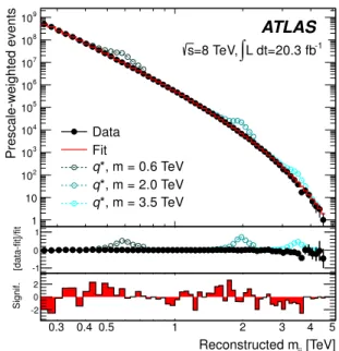
IV. COMPARISON OF THE DIJET MASS SPECTRUM TO A SMOOTH BACKGROUND The observed dijet mass distribution in data, after all selection requirements, is shown in Fig.2. The bin width varies with mass and is chosen to approximately equal the dijet mass resolution derived from simulation of QCD processes. The predictions for an excited quark q∗ with three different mass hypotheses are also shown.
The search for resonances in mjj uses a data-driven
background estimate derived by fitting a smooth func-tional form to the spectrum. An important feature of this functional form is that it allows for smooth back-ground variations, but does not accommodate localized excesses that could indicate the presence of NP signals. In previous studies, ATLAS and other experiments [54] have found that the following function provides a satis-factory fit to the QCD prediction of dijet production:
f (x) = p1(1 − x)p2xp3+p4ln x, (1)
where the piare fit parameters, and x ≡ mjj/
√ s. The uncertainty associated with the stability of the fit is car-ried forward as a nuisance parameter in the statistical analysis.
The functional form was selected using a data set con-sisting of a quarter of the full data, a quantity known to be insensitive to resonant new physics at dijet masses above 1.5 TeV after the previous public result on 13 fb−1 of data [55]. A range of parametrizations were tested on the blinded data set using a k-fold cross-validation
and there was found to be no substantial difference be-tween the standard function of Eq. 1 and higher-order parametrizations, so the function with a simpler form and a published precedent was selected. The χ2-value
of the fit to the blinded data set was 37 for 56 degrees of freedom using the parameterisation of Eq. 1. The fit function showed good agreement to both the fully simulated dijet mass spectrum obtained from the sim-ulated Pythia 8.160 QCD multijet events mentioned in Sec.III, corrected for next-to-leading-order effects using the NLOJET++ v4.1.3 program [56,57] as described in Ref. [11], and from a large-statistics sample of generator-level events, for which the chi2 of the fit was 58 for 55 degrees of freedom. While the number of data events is matched or surpassed by the number of fully simulated events starting from dijet masses of roughly 2 TeV, the generator-level statistics is sufficient to reproduce that of data. The χ2-value of the fit to data shown in Fig. 2 is 79 for 56 degrees of freedom.
Prescale-weighted events 1 10 2 10 3 10 4 10 5 10 6 10 7 10 8 10 9 10 [data-fit]/fit -1 0 1 [TeV] jj Reconstructed m 0.3 0.4 0.5 1 2 3 4 5 Signif. -20 2 ATLAS -1 L dt=20.3 fb
∫
=8 TeV, s Data Fit *, m = 0.6 TeV q *, m = 2.0 TeV q *, m = 3.5 TeV qFigure 2. The reconstructed dijet mass distribution (filled points) fitted with a smooth functional form (solid line). Predictions for three q∗ masses are shown above the back-ground. The central panel shows the relative difference be-tween the data and the background fit with overlaid predic-tions for the same q∗masses. The bin-by-bin significance of the data-background difference considering statistical uncer-tainties only is shown in the bottom panel.
The center panel of Fig.2shows the relative difference between the data and the background fit, and overlays the shapes that would be expected in the presence of three sample q∗signals. The bottom panel of Fig.2shows the significance of the difference between the data and the fit in each bin. The significance is calculated taking only statistical uncertainties into account, and assuming that the data follow a Poisson distribution with the expected value given by the fit function.
For each bin a p-value is determined by assessing the probability of a background fluctuation leading to a num-ber of events higher than or equal to the observed excess, or lower than or equal to the observed deficit. This p-value is converted to a significance in terms of an equiv-alent number of standard deviations (the z-value) [58]. Where there is an excess (deficit) in data in a given bin, the significance is plotted as positive (negative).2 To test
the degree of consistency between the data and the fitted background, the p-value of the fit is determined by cal-culating the χ2-value from the data and comparing this
result to the χ2distribution obtained from pseudoexper-iments drawn from the background fit, as described in a previous publication [11]. The resulting p-value is 0.027. The BumpHunter algorithm [59,60] is used to estab-lish the presence or absence of a narrow resonance in the dijet mass spectrum, as described in greater detail in previous publications [11,12]. Starting with a two-bin window, the algorithm increases the signal window and shifts its location until all possible bin ranges, up to the widest window corresponding to half the mass range spanned by the data, are tested. The most significant excess of data above the smooth spectrum (“bump”) is defined by the set of bins over which the integrated excess of data over the fit prediction has the smallest probabil-ity of arising from a background fluctuation, assuming Poisson statistics.
The BumpHunter algorithm accounts for the so-called “look-elsewhere effect” [61], by performing a se-ries of pseudoexperiments drawn from the background estimate to determine the probability that random fluc-tuations in the background-only hypothesis would create an excess anywhere in the spectrum at least as signifi-cant as the one observed. Furthermore, to prevent any NP signal from biasing the background estimate, if the most significant local excess from the background fit has a p-value smaller than 0.01, the corresponding region is excluded and a new background fit is performed. The exclusion is then progressively widened bin by bin until the p-value of the remaining fitted region is acceptable. No such exclusion is needed for the current data set.
The most significant discrepancy identified by the BumpHunter algorithm in the observed dijet mass dis-tribution in Fig. 2 is a seven-bin excess in the interval 390–599 GeV. The probability of observing an excess at least as large somewhere in the mass spectrum for a background-only hypothesis is 0.075, corresponding to a z-value of 1.44σ. To conclude, this test shows no evidence for a resonant signal in the observed mjj spectrum.
2 In mass bins with small expected number of events, where the
observed number of events is similar to the expectation, the Pois-son probability of a fluctuation at least as high (low) as the ob-served excess (deficit) can be greater than 50%, as a result of the asymmetry of the Poisson distribution. Since these bins have too few events for the significance to be meaningful, these bins are drawn with zero content.
V. SIMULATION OF HYPOTHETICAL NEW PHENOMENA
In the absence of any significant signals indicating the presence of phenomena beyond the SM, Bayesian 95% credibility level (C.L.) limits are determined for a number of NP hypotheses that would produce localized excesses. Samples for NP models are produced by a variety of event generators. The partons originating from the initial 2 → 2 matrix elements are passed to Pythia 8.160 with the AU2 tune [45]. Pythia uses pT-ordered parton
show-ers to model additional radiation in the leading-logarithm approximation [62]. Multiple parton interactions [63], as well as fragmentation and hadronization based on the Lund string model [64], are also simulated. Renormal-ization and factorRenormal-ization scales for the NP models are set to the mean pTof the two leading jets.
Excited u- and d- quarks (q∗), one possible
manifesta-tion of quark compositeness, are simulated in all decay modes using the Pythia 8.162 generator, using the CT10 PDF. Excited quarks are assumed to decay to quarks via gauge couplings set to unity, leading to a qg final state approximately 83% of the time (the remaining generated decays involve W/Z or γ emission). The acceptance, de-fined as the fraction of generated events passing all re-construction steps and the analysis selection described in Sec.III using jets reconstructed from stable particles3
excluding muons and neutrinos, is approximately 58%. The largest reduction in acceptance arises from the ra-pidity selection criteria.
The color-octet scalar model describes the produc-tion of exotic colored resonances (s8). MadGraph 5 (v1.5.5) [65] with the MSTW2008LO PDF [66] is em-ployed to generate parton-level events at leading-order approximation. Parton showering and nonperturbative effects are simulated with Pythia 8.170. Color-octet scalars can decay into two gluons and can then have a broader mass distribution and larger tails than reso-nances decaying to quarks. For resoreso-nances produced by this model, the acceptance ranges from 61% to 63%.
The production of heavy charged gauge bosons, W0, has been sought through decays to q ¯q0. The specific model (sequential Standard Model, or SSM [26,27]) used in this study assumes that the W0 has V − A SM cou-plings but does not include interference between the W0 and the W , leading to a branching ratio to dijets of 75%. The W0 signal sample is simulated with the Pythia 8.165 event generator using the MSTW2008LO PDF. Instead of the LO cross section values, the next-to-next-to-leading-order cross section values calculated with the MSTW2008NNLO PDF are used in this analysis, as detailed in [67] and references therein. The acceptance for W0 bosons decaying to quarks ranges from 48% at
3A stable particle is defined as one that has a lifetime longer than
masses below 1200 GeV to 40% at 3200 GeV, driven by the rapidity selection criteria. At high W0masses, the ac-ceptance decreases due to PDF suppression effects caus-ing the reconstructed dijet invariant mass to fall below the 250 GeV cut.
A new excited W∗ boson [31,32] is generated through a simplified model [30] in the CalcHEP 3.4.2 genera-tor, in combination with the MSTW2008LO PDF and Pythia 8.165 for the simulation of nonperturbative ef-fects. The sine of the mixing angle in this model (sinφX)
is set to zero, producing leptophobic decays of the W∗ that are limited to quarks. With sinφX = 1, a leptophilic
W∗ would instead be produced with branching ratios di-vided equally between quarks (3 families × 3 flavors × 8.3% BR = 75%) and leptons (3 families × 8.3% BR = 25%). The angular distribution of the W∗ differs from that of the other signals under study, preferring decays with a wider separation in y. The acceptance for both leptophobic and leptophilic W∗ spans 25% to 27%.
A model for quantum black holes (QBH) that decay to two jets is simulated using both the BlackMax [68] and the Qbh [69] generators, to produce a simple two-body final-state scenario of quantum gravitational effects at the fundamental Planck scale MD, with n = 6 extra
spatial dimensions in the context of the ADD model [70]. In this model, the Planck scale is set equal to the thresh-old mass for the quantum black hole production mth.
These QBH models are used as benchmarks to represent any quantum gravitational effect that produces events containing dijets. The PDF used for the generation and parton shower of BlackMax is CT10, while the Qbh samples employ the MSTW2008LO PDF. In the mass range considered, the branching ratio of QBH to dijets is above 85% and the acceptance is between 52% and 55% for BlackMax and 54%–56% for Qbh. nonperturbative effects for events coming from both event generators are simulated with Pythia 8.170.
Further information on cross sections, branching ra-tio to dijets and acceptances for the benchmark models under consideration can be found in HepData [71].
All MC signal samples except for the excited quark signals are passed through a fast detector simulation [72] with the jet calibration appropriately corrected to full simulation. The excited quark signals are simulated us-ing Geant4 within the ATLAS simulation infrastruc-ture [47].
VI. LIMITS ON NEW RESONANT PHENOMENA FROM THE mjj DISTRIBUTION
The Bayesian method used for the limit setting is doc-umented in Ref. [11] and implemented using the Bayesian Analysis Toolkit [73]. Limits on the cross section times acceptance, σ ×A, are set at the 95% C.L. for the NP sig-nal as a function of mNP, using a prior constant in signal
strength and Gaussian priors for the nuisance parameters due to the systematic uncertainties under consideration.
The full template shape is considered in the limit-setting procedure, both in the fits to the data performed during the marginalization procedure4and in the likelihood for
the determination of the 95% C.L. limit. The limit on σ × A from data is interpolated linearly on the x axis and logarithmically on the y axis between the mass points to create a continuous curve in signal mass. The exclusion limit on the mass (or energy scale) of the given NP sig-nal occurs at the value of the sigsig-nal mass where the limit on σ × A from data is the same as the theoretical value, which is derived by interpolation between the generated mass values. This form of analysis is applicable to all resonant phenomena where the NP couplings are strong compared to the scale of perturbative QCD at the signal mass, so that interference between these terms can be neglected.
As in previous dijet resonance analyses, limits on dijet resonance production are also determined using a collec-tion of hypothetical signal shapes that are assumed to be Gaussian-distributed in mjj. Signal shape templates
are generated with means (mG) ranging from 200 GeV to
4.0 TeV and with standard deviations (σG) corresponding
to the dijet mass resolution estimated from MC simula-tion and ranging from 7% to 15% of the mean.5 For
fur-ther information on the mass resolution, see AppendixB. An additional set of limits with minimal model as-sumptions is added to this publication. For particles with a nonzero natural width generated at masses close to the collision energy, the parton luminosity favors lower-mass collisions. This creates an asymmetric resonance not well represented by a Gaussian distribution. To handle this scenario, Breit-Wigner signals of fixed intrinsic widths (0.5% to 5% of the resonance mass) are generated and multiplied by the parton luminosities for different ini-tial states (qq, qg, gg and q ¯q) according to the CT10 PDF. Effects of parton shower and nonperturbative ef-fects are estimated using HERWIG++2.6.3 [74,75] and convoluted with the signal shape.
The detector resolution is accounted for by convolv-ing the signal shape with a Gaussian function of width equal to the detector resolution at each signal mass. The result is then truncated below 250 GeV due to the di-jet mass cut. This produces a signal template shape that is still generic but more likely to match the forms visible in actual physical processes. The effect on the shape of the signal template originating from the y∗ cut is not simulated in the signal templates used for these limits, due to the possible model dependence of the
an-4The NP signal distribution is added to the binned data spectrum,
and the parameters of the background function are extracted by fitting the combined distribution to a five-parameter function, where the fifth parameter is proportional to the signal strength.
5 Limits are determined only for those Gaussian resonances whose
means fall more than 2σ from either edge of the data to pre-serve the stability of the background estimation, so the limits from wider signals include fewer mass points near the ends of the range.
gular distribution of the considered NP process.6 Tests of the benchmark model-specific templates indicate that the combined effect of the y and y∗ acceptance requirement is constant within 20% as a function of the dijet mass, with the largest discrepancies outside the mass peak.
A. Systematic uncertainties in limit setting The effects of several systematic uncertainties are con-sidered when setting limits on new phenomena. These are incorporated into the Bayesian marginalization limit setting procedure using Gaussian priors, with one nui-sance parameter for each uncertainty. They are listed below.
(1) Choice of fitting function: a tenfold cross valida-tion [76] using the full data set shows that the background is also well described when introducing an additional de-gree of freedom to Eq. (1),
f (x) = p1(1 − x)p2xp3+p4ln x+p5(ln x) 2
. (2) The χ2-value of this five-parameter function fit to data
is 45 for 57 degrees of freedom. Since the two fit func-tions provide background estimates that differ beyond statistical uncertainties, an additional uncertainty is in-troduced due to the choice of fitting function. The differ-ence between the two background estimates is treated as a one-sided nuisance parameter, with a Gaussian prior centered at zero corresponding to the background esti-mate from Eq. (1) and truncated to one-σ corresponding to the background estimate from Eq. (2). The marginal-ized posterior indicates a preference for the alternative function.
(2) Background fit quality: the uncertainty on the background parametrization from the fit is estimated by refitting bin-by-bin Poisson fluctuations of the data, as described in Ref. [77]. The resulting uncertainty is calcu-lated by refitting a large number of pseudoexperiments drawn from the data, and defining the fit error from the variation in fit results in each bin: ±1σ in the uncertainty corresponds to the central 68% of pseudoexperiment fit values in the bin.
(3) Jet energy scale: shifts to the jet energy due to the various jet energy scale (JES) uncertainty compo-nents are propagated separately through the analysis of the signal templates. Changes in both shape and accep-tance due to the JES uncertainty in the simulated signal templates are considered in the limit setting. Combined, the JES uncertainty shifts the resonance mass peaks by less than 3%: this is the JES shift used for Gaussian and Breit-Wigner limits.
6 If a flat distribution in the jet polar angle in the center-of-mass
rest frame for the new particle is assumed for the NP model, the acceptance can be calculated analytically and it amounts to roughly 56% for all considered dijet masses.
(4) Luminosity: a 2.8% uncertainty [15] is applied to the overall normalization of the signal templates.
(5) Theoretical uncertainties: the uncertainty on the signal acceptance for the model-dependent limits due to the choice of PDF is derived employing the PDF4LHC recommendation [78] using the envelope of the error sets of the NNPDF 2.1 [79] and MSTW2008LO. Renormal-ization and factorRenormal-ization scale uncertainties on the signal acceptance are considered for the W0 and s8 signals but found negligible. Since the W0 cross section estimation used in this analysis includes NNLO corrections, the un-certainties on cross section due to variations of the renor-malization and factorization scales, the choice of PDF, and PDF+αs variations on the theoretical cross section
are considered as well.
The effect of the jet energy resolution uncertainty is found to be negligible. Similarly, effects due to jet re-construction efficiency and jet angular resolution lead to negligible uncertainties. [TeV] * q m 1 2 3 4 5 [pb] A × σ -3 10 -2 10 -1 10 1 10 2 10 3 10 ATLAS * q
Observed 95% CL upper limit Expected 95% CL upper limit 68% and 95% bands -1 L dt = 20.3 fb
∫
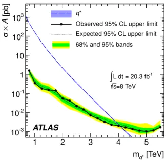
=8 TeV sFigure 3. Observed (filled circles) and expected 95% C.L. upper limits (dotted line) on σ × A for excited quarks as a function of particle mass. The green and yellow bands rep-resent the 68% and 95% contours of the expected limit. The dashed curve is the theoretical prediction of σ × A. The un-certainty on the nominal signal cross section due to the beam energy uncertainty is also displayed as a band around the the-ory prediction. The observed (expected) mass limit occurs at the crossing of the dashed σ × A curve with the observed (expected) 95% C.L. upper limit curve.
B. Constraints on NP benchmark models The resulting limits for excited quarks are shown in Fig.3. The expected lower mass limit at 95% C.L. for q∗ is 3.98 TeV, and the observed limit is 4.06 TeV. The limits for color-octet scalars are shown in Fig. 4. The
[TeV] 8 s m 1 2 3 4 [pb] A × σ -2 10 -1 10 1 10 2 10 3 10 ATLAS 8 s
Observed 95% CL upper limit Expected 95% CL upper limit 68% and 95% bands -1 L dt = 20.3 fb
∫
=8 TeV sFigure 4. Observed (filled circles) and expected 95% C.L. upper limits (dotted line) on σ × A for color-octet scalars as a function of particle mass. The green and yellow bands represent the 68% and 95% contours of the expected limit. The dashed curve is the theoretical prediction of σ × A. The uncertainty on the nominal signal cross section due to the beam energy uncertainty is also displayed as a band around the theory prediction. The observed (expected) mass limit occurs at the crossing of the dashed σ × A curve with the observed (expected) 95% C.L. upper limit curve.
expected mass limit at 95% C.L. is 2.80 TeV, and the observed limit is 2.70 TeV.
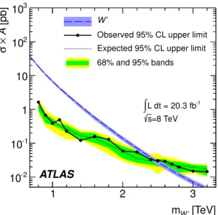
The limits for heavy charged gauge bosons, W0, are shown in Fig.5. The expected mass limit at 95% C.L. is 2.51 TeV, and the observed limit is 2.45 TeV.
The limits for the excited W∗ boson are shown in Fig.6. The plot shows the observed and expected lim-its calculated for a leptophobic W∗ but includes the-ory curves for both leptophobic and nonleptophobic W∗
given that the acceptances for the two samples are the same to within 1%. The expected mass limit for the leptophobic model at 95% C.L. is 1.95 TeV and the ob-served limit is 1.75 TeV. The expected mass limit for the nonleptophobic model at 95% C.L. is 1.66 TeV and the observed limit is 1.65 TeV.
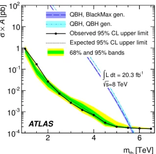
The limits for black holes generated using Qbh and BlackMax are shown in Fig. 7. The observed limit is consistent between the two generators, but the cross sec-tions differ, hence the difference in the mass limit. The observed limits for the two models have visually matching shapes and normalizations, so only one (BlackMax) is selected for display. The limits for both models are, how-ever, computed separately and recorded. The expected mass limit for Qbh black holes at 95% C.L. is 5.66 TeV, and the observed limit is 5.66 TeV. For BlackMax black holes, the expected limit at 95% C.L. is 5.62 TeV and the observed limit is 5.62 TeV. Above ∼4.5 TeV the
[TeV] ’ W m 1 2 3 [pb] A × σ -2 10 -1 10 1 10 2 10 3 10 ATLAS ’ W
Observed 95% CL upper limit Expected 95% CL upper limit 68% and 95% bands -1 L dt = 20.3 fb
∫
=8 TeV sFigure 5. Observed (filled circles) and expected 95% C.L. upper limits (dotted line) on σ × A for heavy vector bosons as a function of particle mass. The green and yellow bands represent the 68% and 95% contours of the expected limit. The dashed curve is the theoretical prediction of σ × A. The uncertainty on the nominal signal cross section due to the beam energy uncertainty is also displayed as a band around the theory prediction. Additionally the uncertainty on the calculation of the next-to-next-to-leading order cross section is shown around the theory line. The observed (expected) mass limit occurs at the crossing of the dashed σ × A curve with the observed (expected) 95% C.L. upper limit curve.
served and expected limits are driven by the absence of any observed data events, leading to identical observed and expected mass limits.
Although the search phase of the analysis starts at 250 GeV, σ × A exclusion limits on benchmark NP models are set starting at 800 GeV for the q∗, s8, and W0 mod-els, and at 1500 GeV for the W∗model. In the first three cases, this ensures that the rapid increase in the delayed stream statistics from 800 GeV onwards does not shift the search to be more sensitive to the tails of the model, rather than to its peak. In the W∗model, the limited ac-ceptance distorts the peak shape below 1500 GeV so that it cannot be adequately treated as a resonance. Exclu-sion limits on quantum black holes are set starting from 1 TeV in light of the large cross section and of previous exclusion limits [77,80].
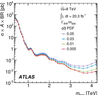
C. Generic resonance limits on dijet production The resulting limits on σ × A for the Gaussian tem-plate shape are shown in Fig.8. Limits resulting from the convolution of Breit-Wigner signals of different intrinsic widths (ΓBW) with the appropriate parton distribution
[TeV] * W m 1.5 2 2.5 3 3.5 [pb] A × σ -3 10 -2 10 -1 10 1 10 2 10 ATLAS =0) X φ * (sin W Leptophobic =1) X φ * (sin W Leptophilic
Observed 95% CL upper limit Expected 95% CL upper limit 68% and 95% bands -1 L dt = 20.3 fb
∫
=8 TeV sFigure 6. Observed (filled circles) and expected 95% C.L. up-per limits (dotted line) on σ × A for leptophobic and nonlep-tophobic excited vector bosons W∗ as a function of particle mass. The green and yellow bands represent the 68% and 95% contours of the expected limit. The dashed curve is the theoretical prediction of σ × A. The uncertainty on the nom-inal signal cross section due to the beam energy uncertainty is also displayed as a band around the theory prediction. The observed (expected) mass limit occurs at the crossing of the dashed σ × A curve with the observed (expected) 95% C.L. upper limit curve.
tector resolution are shown in Figs. 9 and 10. For the initial Breit-Wigner signal the following nonrelativistic function was chosen:
f (x, µ, Γ) = 1 2π
Γ
(x − µ)2+ (Γ2/4)
, where µ and Γ are the mass and the width of the res-onance. The use of a relativistic Breit-Wigner signal for the resonance line shape may lead to different limits than the ones derived using the nonrelativistic approximation above. Parton showers and nonperturbative effects have been simulated using HERWIG++2.6.3, which gives a more conservative limit with respect to what is obtained from Pythia.
The difference in shapes between the two Breit-Wigner limits is a result of the much larger low-mass tails result-ing from the gg parton luminosity, which becomes espe-cially pronounced at high masses. The convolution with parton shower and nonperturbative effects enhances this effect further.
For sufficiently narrow resonances, these results may be used to set limits on NP models beyond those con-sidered in the current studies, as described in detail in AppendixA.
It should be noted that these limits will be conservative at high masses with respect to the limits obtained with
[TeV] th m 2 4 6 [pb] A × σ -4 10 -3 10 -2 10 -1 10 1 10 2 10 ATLAS QBH, BlackMax gen. QBH, QBH gen.
Observed 95% CL upper limit Expected 95% CL upper limit 68% and 95% bands -1 L dt = 20.3 fb
∫
=8 TeV sFigure 7. Observed (filled circles) and expected 95% C.L. up-per limits (dotted line) on σ × A for black holes simulated using the Qbh and BlackMax generators as a function of particle mass. The green and yellow bands represent the 68% and 95% contours of the expected limit. The dashed curve is the theoretical prediction of σ × A. The uncertainty on the nominal signal cross section due to the beam energy uncer-tainty is also displayed as a band around the theory predic-tion. The observed (expected) mass limit occurs at the cross-ing of the dashed σ × A curve with the observed (expected) 95% C.L. upper limit curve.
full benchmark templates. This is due to the simplifying assumptions made in their derivation, in particular from the use of a nonrelativistic and mass-independent Breit-Wigner shape.
Gaussian limits should be used when tails from PDF and nonperturbative effects can be safely truncated or neglected. Otherwise, convolved Breit-Wigner signals would be more reliable.
In the case of the Gaussian limits, the signal distri-bution after applying the kinematic selection criteria on y∗, mjj and η of the leading jets (Sec. III) should
ap-proach a Gaussian distribution. The acceptance should include the jet reconstruction efficiency (100% for the current analysis and detector conditions, since inefficien-cies due to calorimeter problems are corrected for in data) and the efficiency with respect to the kinematic selection above. NP models with a width smaller than 5% should be compared to the results with width equal to the ex-perimental resolution only (see AppendixB). For models with a larger width after detector effects, the limit that best matches their width should be used.
[TeV] G m 1 2 3 4 BR [pb]× A × σ -4 10 -3 10 -2 10 -1 10 1 10 2 10 3 10 ATLAS =8 TeV s -1 L dt = 20.3 fb
∫
G /m G σ 0.15 0.10 0.07 ResolutionFigure 8. The 95% C.L. upper limits on σ × A for a sim-ple Gaussian resonance decaying to dijets as a function of the mean mass, mG, for four values of σG/mG, taking into
account both statistical and systematic uncertainties.
[TeV] BW m 1 2 3 4 BR [pb]× A × σ -3 10 -2 10 -1 10 1 10 2 10 3 10 4 10 ATLAS =8 TeV s -1 L dt = 20.3 fb
∫
BW /m BW Γ PDF gg 0.05 0.03 0.01 0.005Figure 9. The 95% C.L. upper limits on σ × A for a Breit-Wigner narrow resonance produced by a gg initial state de-caying to dijets and convolved with PDF effects, dijet mass acceptance, parton shower and nonperturbative effects and detector resolution, as a function of the mean mass, mBW,
for different values of intrinsic width over mass (ΓBW/mBW),
taking into account both statistical and systematic uncertain-ties. [TeV] BW m 1 2 3 4 BR [pb]× A × σ -3 10 -2 10 -1 10 1 10 2 10 3 10 4 10 ATLAS =8 TeV s -1 L dt = 20.3 fb
∫
BW /m BW Γ PDF q q 0.05 0.03 0.01 0.005Figure 10. The 95% C.L. upper limits on σ × A for a Breit-Wigner narrow resonance produced by a q ¯q initial state de-caying to dijets and convolved with PDF effects, dijet mass acceptance, parton shower and nonperturbative effects and detector resolution, as a function of the mean mass, mBW,
for different values of intrinsic width over mass (ΓBW/mBW),
taking into account both statistical and systematic uncertain-ties.
VII. CONCLUSIONS
In the 2012 running of the ATLAS experiment at the LHC, the collision energy was raised from 7 TeV to 8 TeV, accompanied by a more than fourfold increase in inte-grated luminosity. The higher energy, and the associated rise in parton luminosity for high masses, have increased the sensitivity of the search and its mass reach for various model hypotheses. In addition, novel trigger techniques have been employed to extend the search to low dijet masses. The data sample used in the current analysis consists of 20.3 fb−1 of pp collision data at√s = 8 TeV,
and the resulting dijet mass distribution extends from 250 GeV to approximately 4.5 TeV.
No resonancelike features are observed in the dijet mass spectrum. This analysis places limits on the cross section times acceptance at the 95% credibility level on the mass or energy scale of a variety of hypotheses for physics phenomena beyond the Standard Model.
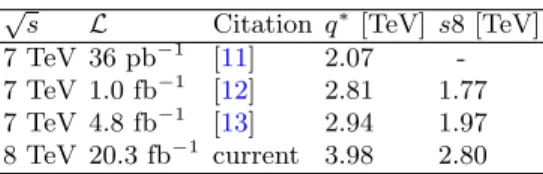
To illustrate the typical increases in sensitivity to new phenomena at the LHC up to the end of 2012 running, Table II shows the history of expected limits from AT-LAS studies using dijet resonance analysis of two bench-mark models, excited quarks and color-octet scalars. The limits set by this analysis on excited quarks, color-octet scalars, heavy W0 bosons, chiral W∗ bosons, and quan-tum black holes, are summarized in TableI.
Model and final state 95% C.L. Limits [TeV] expected observed q∗→ qg 3.98 4.06 s8 → gg 2.80 2.70 W0→ q ¯q0 2.51 2.45 Leptophobic W∗→ q ¯q0 1.95 1.75 Leptophilic W∗→ q ¯q0 1.66 1.65 Qbh black holes 5.66 5.66 (q and g decays only)
BlackMax black holes 5.62 5.62 (all decays)
Table I. The 95% C.L. lower limits on the masses and energy scales of the models examined in this study. All limit analy-ses are Bayesian, with statistical and systematic uncertainties included.
√
s L Citation q∗[TeV] s8 [TeV] 7 TeV 36 pb−1 [11] 2.07 -7 TeV 1.0 fb−1 [12] 2.81 1.77 7 TeV 4.8 fb−1 [13] 2.94 1.97 8 TeV 20.3 fb−1 current 3.98 2.80
Table II. ATLAS previous and current expected 95% C.L. upper limits [TeV] on excited quarks and color-octet scalars.
ACKNOWLEDGMENTS
We thank CERN for the very successful operation of the LHC, as well as the support staff from our institutions without whom ATLAS could not be operated efficiently. We acknowledge the support of ANPCyT, Argentina; YerPhI, Armenia; ARC, Australia; BMWF and FWF, Austria; ANAS, Azerbaijan; SSTC, Belarus; CNPq and FAPESP, Brazil; NSERC, NRC and CFI, Canada; CERN; CONICYT, Chile; CAS, MOST and NSFC, China; COLCIENCIAS, Colombia; MSMT CR, MPO CR and VSC CR, Czech Republic; DNRF, DNSRC and Lundbeck Foundation, Denmark; EPLANET, ERC and NSRF, European Union; IN2P3-CNRS, CEA-DSM/IRFU, France; GNSF, Georgia; BMBF, DFG, HGF, MPG and AvH Foundation, Germany; GSRT and NSRF, Greece; RGC, Hong Kong SAR, China; ISF, MINERVA, GIF, I-CORE and Benoziyo Center, Israel; INFN, Italy; MEXT and JSPS, Japan; CNRST, Mo-rocco; FOM and NWO, Netherlands; BRF and RCN, Norway; MNiSW and NCN, Poland; GRICES and FCT, Portugal; MNE/IFA, Romania; MES of Russia and ROSATOM, Russian Federation; JINR; MSTD, Serbia; MSSR, Slovakia; ARRS and MIZˇS, Slovenia; DST/NRF, South Africa; MINECO, Spain; SRC and Wallenberg Foundation, Sweden; SER, SNSF and Cantons of Bern and Geneva, Switzerland; NSC, Taiwan; TAEK, Turkey; STFC, the Royal Society and Leverhulme Trust, United Kingdom; DOE and NSF, United States of America.
The crucial computing support from all WLCG part-ners is acknowledged gratefully, in particular from CERN and the ATLAS Tier-1 facilities at TRIUMF (Canada), NDGF (Denmark, Norway, Sweden), CC-IN2P3 (France), KIT/GridKA (Germany), INFN-CNAF (Italy), NL-T1 (Netherlands), PIC (Spain), ASGC (Tai-wan), RAL (UK) and BNL (USA) and in the Tier-2 fa-cilities worldwide.
Appendix A: Suggested procedure for setting limits on generic NP models
1. Setting limits for NP models with a Gaussian shape
The following detailed procedure is appropriate for set-ting limits involving resonances that are approximately Gaussian near the core, and with tails that are much smaller than the background. The results of Fig. 8 are provided in tables on HepData.
(1) Generate an MC sample of a hypothetical new par-ticle with mass set to M . nonperturbative effects should be included in the event generation. Apply the kinematic selection on the parton η, pT, and |y∗| used in this
anal-ysis, as in Sec.III.
(2) Smear the signal mass distribution to reflect the detector resolution. The smearing factors derived from
full ATLAS simulation of QCD dijet events can be taken from Fig.11.
(3) Since a Gaussian signal shape has been assumed in determining the limits, any long tails in the reconstructed mjj should be removed in the sample under study. The
recommendation (based on optimization using q∗ tem-plates) is to retain events with mjj between 0.8M and
1.2M . The mean mass, m, should be recalculated for this truncated signal.
(4) The fraction of MC events surviving the first four steps determines the modified acceptance, A.
(5) From the table in HepData, select mG so that
mG = m. If the exact value of m is not among the
listed values of mG, check the limit for the two values
of mG that are directly above and below m, and use the
larger of the two limits to be conservative.
(6) To retain enough of the information in the full signal template, and at the same time reject tails that would invalidate the Gaussian approximation, the fol-lowing truncation procedure is recommended. For this mass point, choose a value of σG/mG such that the
re-gion within ±2σG is well contained in the (truncated)
mass range. For the q∗case a good choice is σG= (1.2M
-0.8M )/5 so that 95% of the Gaussian spans 4×(0.4/5)M . Use this value to pick the closest σG/mG value, rounded
up to be conservative.
(7) Compare the tabulated 95% C.L. upper limit cor-responding to the chosen mG and σG/mG values to the
σ × A obtained from the theoretical cross section of the model multiplied by the acceptance defined in step (4) above and taking into account its branching ratio into dijets.
2. Setting limits for NP models with a Breit-Wigner shape, accounting for PDF effects The following detailed procedure is appropriate for setting limits involving resonances that approximate a Breit-Wigner (BW) shape and extend with a low-mass tail due to effects of parton luminosity. For signals that are very narrow or whose tails deviate significantly from a BW, a truncation of the signal template suggested in the Gaussian limits in Sec.A 1might be more appropri-ate. The results of Figs.9and10are provided in Tables I and II on HepData.
(1) Generate a hypothetical new particle, with mass set to M and intrinsic width Γ. As the PDF used to obtain those limits is CT10, the same choice is recommended for the event generation. nonperturbative effects should be simulated after the hard scattering.
(2) Smear the signal mass distribution to reflect the detector resolution. The smearing factors for the dijet mass are derived from full ATLAS simulation and can be taken from Fig.11.
(3) The kinematic selection detailed in Sec.IIIshould be applied to the simulated events. It should be checked at this point that the shape of the template after the
y∗ < 0.6 cut does not change significantly. For example, in a simple model with a flat distribution for the cosine of the polar angle of the jets in the rest frame of the resonance (cos θ∗) that decays into two back-to-back jets (ylead≈ −ysublead), a cut on |y∗| = 0.5∗|ylead−ysublead| <
0.6 imposes a cut on the unboosted rapidity distribution (|ylead,sublead| < 0.6). In the mass ranges investigated,
this corresponds to a more stringent constraint than the ηBW < 2.8 acceptance correction, leading to an
accep-tance of ∼ 0.5 that does not depend on dijet mass. Devia-tions from a flat acceptance of up to 20% can be observed in the tails of models with different angular distributions (q∗, s8, W0).
(4) The fraction of generated events surviving the first three steps determines the signal acceptance, A.
(5) From the tables available in HepData, select the one corresponding to the production mode for the new resonance (gluon-gluon, gluon-quark, quark-quark or quark-antiquark) as the parton luminosities and hence the signal shapes differ.
(6) Compare the tabulated 95% C.L. upper limit cor-responding to the chosen M and Γ/M values to the σ ×A obtained from the theoretical cross section of the model, multiplied by the acceptance defined in step (3) above and taking into account its branching ratio into dijets.
If the exact values of M and Γ/M are not among the listed values of mBW and ΓBW/mBW, check the limit for
the two values of mBWthat are directly above and below
M , and use the more conservative of the two limits.
Appendix B: Dijet mass resolution
The dijet mass resolution in Fig. 11 is derived from fully simulated QCD Monte Carlo, generated with Pythia 8.175 [43], using the AU2 tune obtained from ATLAS data [45] using the analysis selection detailed in Sec. III. The dijet mass resolution σmjj/mjj is 8% at
mjj '250 GeV, falls to 4% at 2 TeV, and approaches 4%
at mjj of 3 TeV and above, and it is interpolated linearly
between the bin centers.
Appendix C: Signal template shapes
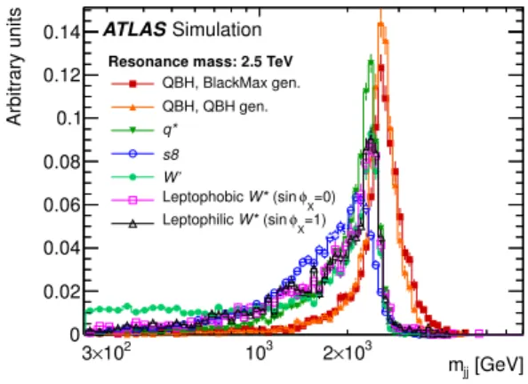
For ease of comparison of the shapes of different signals used in this paper, the various signal template shapes are overlaid in Fig. 12 for the mass point of 2.5 TeV, after normalizing to the same area.
[GeV] jj m 2 10 × 2 103 2×10³ jj /mjj m σ 0.02 0.04 0.06 0.08 0.1 0.12 0.14 ATLASSimulation Pythia8 QCD
Figure 11. Dijet mass resolution obtained from fully simu-lated Pythia QCD Monte Carlo Pythia 8.175 [43], with the AU2 tune obtained from ATLAS data [45]. The dijet mass resolution is interpolated linearly between the bin centers.
[GeV] jj m 2 10 × 3 103 2×10³ Arbitrary units 0 0.02 0.04 0.06 0.08 0.1 0.12 0.14
Resonance mass: 2.5 TeV
QBH, BlackMax gen. QBH, QBH gen. q* s8 W’ =0) X φ (sin W* Leptophobic =1) X φ (sin W* Leptophilic ATLAS Simulation
Figure 12. Dijet invariant mass for models corresponding to a resonance mass of 2.5 TeV. All distributions are normalized to the same area.
REFERENCES
[1] G. Arnison et al. (UA1 Collaboration), Phys. Lett. B 136, 294 (1984).
[2] P. Bagnaia et al. (UA2 Collaboration),Phys. Lett. B 144, 283 (1984).
[3] T. Aaltonen et al. (CDF Collaboration),Phys. Rev. D 79, 112002 (2009),arXiv:0812.4036 [hep-ex].
[4] V. Abazov et al. (D0 Collaboration), Phys. Rev. Lett. 103, 191803 (2009),arXiv:0906.4819 [hep-ex].
[5] ATLAS Collaboration, Phys. Rev. Lett. 105, 161801 (2010),arXiv:1008.2461 [hep-ex].
[6] ATLAS Collaboration, Phys. Lett. B 694, 327 (2011), arXiv:1009.5069 [hep-ex].
[7] CMS Collaboration, Phys. Rev. Lett. 105, 211801 (2010),arXiv:1010.0203 [hep-ex].
[8] CMS Collaboration, Phys. Rev. Lett. 105, 262001 (2010),arXiv:1010.4439 [hep-ex].
[9] CMS Collaboration, Phys. Rev. Lett. 106, 201804 (2011),arXiv:1102.2020 [hep-ex].
[10] CMS Collaboration, Phys. Lett. B 704, 123 (2011), arXiv:1107.4771 [hep-ex].
[11] ATLAS Collaboration, New J. of Phys. 13, 053044 (2011),arXiv:1103.3864 [hep-ex].
[12] ATLAS Collaboration, Phys. Lett. B 708, 37 (2012), arXiv:1108.6311 [hep-ex].
[13] ATLAS Collaboration,J. High Energy Phys. 2013, 029 (2013),arXiv:1210.1718 [hep-ex].
[14] CMS Collaboration, Phys. Rev. D 87, 114015 (2013), arXiv:1302.4794 [hep-ex].
[15] ATLAS Collaboration,Eur. Phys. J. C 73, 2518 (2013), arXiv:1302.4393 [hep-ex].
[16] U. Baur, I. Hinchliffe, and D. Zeppenfeld,Int. J. Mod. Phys. A 2, 1285 (1987).
[17] U. Baur, M. Spira, and P. M. Zerwas,Phys. Rev. D 42, 815 (1990).
[18] P. H. Frampton and S. L. Glashow,Phys. Lett. B , 157 (1987).
[19] P. H. Frampton and S. L. Glashow,Phys. Rev. Lett. 58, 2168 (1987).
[20] J. Bagger, C. Schmidt, and S. King,Phys. Rev. D 37, 1188 (1988).
[21] T. Han, I. Lewis, and Z. Liu,J. High Energy Phys. 12, 085 (2010),arXiv:1010.4309 [hep-ph].
[22] H. Georgi, E. E. Jenkins, and E. H. Simmons, Nucl. Phys. B 331, 541 (1990).
[23] C. Grojean, E. Salvioni, and R. Torre,J. High Energy Phys. 1107, 002 (2011),arXiv:1103.2761 [hep-ph]. [24] M. Cvetic and J. C. Pati,Phys. Lett. B 135, 57 (1984). [25] Y. Mimura and S. Nandi,Phys. Lett. B 538, 406 (2002),
arXiv:hep-ph/0203126 [hep-ph].
[26] G. Altarelli, B. Mele, and M. Ruiz-Altaba,Z. Phys. C 45, 109 (1989).
[27] G. Altarelli, B. Mele, and M. Ruiz-Altaba,Z. Phys. C 47, 676 (1990).
[28] CMS Collaboration, Phys. Lett. B 701, 160 (2011), arXiv:1103.0030 [hep-ex].
[29] ATLAS Collaboration, Phys. Lett. B 705, 28 (2011), arXiv:1108.1316 [hep-ex].
[30] M. Chizhov, Phys. Part. Nucl. Lett. 8, 512 (2011), arXiv:1005.4287 [hep-ph].
[31] M. Chizhov and G. Dvali,Phys. Lett. B 703, 593 (2011). [32] M. Chizhov, V. Bednyakov, and J. Budagov, Phys.
Atom. Nucl. 75, 90 (2012).
[33] M. Chizhov, V. Bednyakov, and J. Budagov, (2011), arXiv:1106.4161 [hep-ph].
[34] L. A. Anchordoqui, J. L. Feng, H. Goldberg, and A. D. Shapere,Phys. Lett. B 594, 363 (2004), arXiv:hep-ph/0311365 [hep-ph].
[35] P. Meade and L. Randall,J. High Energy Phys. 0805, 003 (2008),arXiv:0708.3017 [hep-ph].
[36] X. Calmet, W. Gong, and S. D. Hsu,Phys. Lett. B 668, 20 (2008),arXiv:0806.4605 [hep-ph].
[37] D. M. Gingrich, J. Phys. G 37, 105008 (2010), arXiv:0912.0826 [hep-ph].
[38] ATLAS Collaboration,JINST 3, S08003 (2008). [39] W. Lampl et al., Report No. ATL-LARG-PUB-2008-002,
(2010),http://cdsweb.cern.ch/record/1099735.
[40] M. Cacciari, G. P. Salam, and G. Soyez,J. High Energy Phys. 04, 063 (2008),arXiv:0802.1189 [hep-ph].
[41] M. Cacciari and G. P. Salam, Phys. Lett. B 641, 57 (2006),arXiv:hep-ph/0512210 [hep-ph].
[42] ATLAS Collaboration, Report No. ATLAS-CONF-2013-083, (2013),http://cdsweb.cern.ch/record/1570994. [43] T. Sjostrand, S. Mrenna, and P. Z. Skands, Comput.
Phys. Commun. 178, 852 (2008),arXiv:0710.3820 [hep-ph].
[44] H.-L. Lai et al., Phys. Rev. D 82, 074024 (2010), arXiv:1007.2241 [hep-ph].
[45] ATLAS Collaboration, Report No. ATLAS-PUB-2012-003, (2013),http://cdsweb.cern.ch/record/1363300. [46] S. Agostinelli et al. (GEANT4),Nucl. Instrum. Methods
Phys. Res., Sect. A 506, 250 (2003).
[47] ATLAS Collaboration,Eur. Phys. J. C 70, 823 (2010), arXiv:1005.4568 [physics.ins-det].
[48] ATLAS Collaboration, (2014),arXiv:1406.0076 [hep-ex]. [49] ATLAS Collaboration,Eur. Phys. J. C 73, 2306 (2013),
arXiv:1210.6210 [hep-ex].
[50] ATLAS Collaboration,Eur. Phys. J. C 72, 1849 (2012), arXiv:1110.1530 [hep-ex].
[51] V. Lendermann et al.,Nucl. Instr. Meth. Phys. Res. A 604, 707 (2009),arXiv:0901.4118 [hep-ph].
[52] ATLAS Collaboration, Report No. ATLAS-CONF-2012-020, (2012),http://cdsweb.cern.ch/record/1430034. [53] ATLAS Collaboration, Report No.
ATLAS-CONF-2010-054, (2010),http://cdsweb.cern.ch/record/1281311. [54] R. M. Harris and K. Kousouris,Int. J. Modern Phys. 26,
5005 (2011),arXiv:1110.5302 [hep-ph].
[55] ATLAS Collaboration, CERN, (2012), ATLAS-CONF-2012-148.
[56] Z. Nagy,Phys. Rev. Lett. 88, 122003 (2002), arXiv:hep-ph/0110.315 [hep-ph].
[57] S. Catani and M. H. Seymour,Nucl. Phys. B 485, 291 (1997), arXiv:hep-ph/9605323 [hep-ph]; Nucl. Phys. B 510, 503 (1998).
[58] G. Choudalakis and D. Casadei,Eur. Phys. J. Plus 127, 25 (2012),arXiv:1111.2062.
[59] T. Aaltonen et al. (CDF Collaboration),Phys. Rev. D 79, 011101 (2009),arXiv:0809.3781 [hep-ex].
[60] G. Choudalakis, (2011),arXiv:1101.0390 [physics.data-an].
[61] L. Lyons,Ann. Appl. Stat. 2, 887 (2008).
[62] R. Corke and T. Sjostrand,Eur. Phys. J. C 69, 1 (2010), arXiv:1003.2384 [hep-ph].
[63] T. Sjostrand and P. Z. Skands,Eur. Phys. J. C 39, 129 (2005),arXiv:hep-ph/0408302 [hep-ph].
[64] B. Andersson, G. Gustafson, G. Ingelman, and T. Sjos-trand,Phys. Rept. 97, 31 (1983).
[65] J. Alwall, M. Herquet, F. Maltoni, O. Mattelaer, and T. Stelzer, J. High Energy Phys. 2011, 128 (2011), arXiv:1106.0522 [hep-ph].
[66] A. Martin, W. Stirling, R. Thorne, and G. Watt,Eur. Phys. J. C 63, 189 (2009),arXiv:0901.0002 [hep-ph]. [67] ATLAS Collaboration (ATLAS Collaboration), J. High
Energy Phys. 2014, 037 (2014), arXiv:1407.7494 [hep-ex].
[68] D.-C. Dai et al., Phys. Rev. D 77, 076007 (2008), arXiv:0711.3012 [hep-ph].
[69] D. M. Gingrich, Comput. Phys. Commun. 181, 1917 (2010),arXiv:0911.5370 [hep-ph].
[70] N. Arkani-Hamed, S. Dimopoulos, and G. Dvali,Phys. Rev. D 59, 086004 (1999), arXiv:hep-ph/9807344 [hep-ph].
[71] hepdata repository for results in this paper:, http:// hepdata.cedar.ac.uk/view/red6339.
[72] ATLAS Collaboration, Report No. ATL-PHYS-PUB-2010-013, (2010), http://cdsweb.cern.ch/record/1300517.
[73] A. Caldwell, D. Koll´ar, and K. Kr¨oninger, Com-put. Phys. Commun. 180, 2197 (2009),arXiv:0808.2552 [physics.data-an].
[74] G. Corcella, I. Knowles, G. Marchesini, S. Moretti, K. Odagiri, et al., JHEP 0101, 010 (2001), arXiv:hep-ph/0011363 [hep-ph].
[75] G. Marchesini, B. Webber, G. Abbiendi, I. Knowles, M. Seymour, et al., Comput.Phys.Commun. 67, 465 (1992).
[76] R. Kohavi, IJCAI 14, 1137 (1995).
[77] ATLAS Collaboration, Phys. Lett. B 728, 562 (2014), arXiv:1309.3230 [hep-ex].
[78] M. Botje et al., (2011),arXiv:1101.0538 [hep-ph]. [79] R. D. Ball, V. Bertone, F. Cerutti, L. Del
Deb-bio, S. Forte, et al., Nucl. Phys. B 849, 296 (2011), arXiv:1101.1300 [hep-ph].
[80] ATLAS Collaboration, Phys. Rev. Lett. 112, 091804 (2014),arXiv:1311.2006 [hep-ex].
The ATLAS Collaboration
G. Aad84, B. Abbott112, J. Abdallah152, S. Abdel Khalek116, O. Abdinov11, R. Aben106, B. Abi113, M. Abolins89, O.S. AbouZeid159, H. Abramowicz154, H. Abreu153, R. Abreu30, Y. Abulaiti147a,147b, B.S. Acharya165a,165b,a,
L. Adamczyk38a, D.L. Adams25, J. Adelman177, S. Adomeit99, T. Adye130, T. Agatonovic-Jovin13a,
J.A. Aguilar-Saavedra125a,125f, M. Agustoni17, S.P. Ahlen22, F. Ahmadov64,b, G. Aielli134a,134b,
H. Akerstedt147a,147b, T.P.A. ˚Akesson80, G. Akimoto156, A.V. Akimov95, G.L. Alberghi20a,20b, J. Albert170,
S. Albrand55, M.J. Alconada Verzini70, M. Aleksa30, I.N. Aleksandrov64, C. Alexa26a, G. Alexander154,
G. Alexandre49, T. Alexopoulos10, M. Alhroob165a,165c, G. Alimonti90a, L. Alio84, J. Alison31, B.M.M. Allbrooke18, L.J. Allison71, P.P. Allport73, J. Almond83, A. Aloisio103a,103b, A. Alonso36, F. Alonso70, C. Alpigiani75,
A. Altheimer35, B. Alvarez Gonzalez89, M.G. Alviggi103a,103b, K. Amako65, Y. Amaral Coutinho24a, C. Amelung23,
D. Amidei88, S.P. Amor Dos Santos125a,125c, A. Amorim125a,125b, S. Amoroso48, N. Amram154, G. Amundsen23,
C. Anastopoulos140, L.S. Ancu49, N. Andari30, T. Andeen35, C.F. Anders58b, G. Anders30, K.J. Anderson31, A. Andreazza90a,90b, V. Andrei58a, X.S. Anduaga70, S. Angelidakis9, I. Angelozzi106, P. Anger44, A. Angerami35, F. Anghinolfi30, A.V. Anisenkov108, N. Anjos125a, A. Annovi47, A. Antonaki9, M. Antonelli47, A. Antonov97,
J. Antos145b, F. Anulli133a, M. Aoki65, L. Aperio Bella18, R. Apolle119,c, G. Arabidze89, I. Aracena144, Y. Arai65,
J.P. Araque125a, A.T.H. Arce45, J-F. Arguin94, S. Argyropoulos42, M. Arik19a, A.J. Armbruster30, O. Arnaez30,
V. Arnal81, H. Arnold48, M. Arratia28, O. Arslan21, A. Artamonov96, G. Artoni23, S. Asai156, N. Asbah42,
A. Ashkenazi154, B. ˚Asman147a,147b, L. Asquith6, K. Assamagan25, R. Astalos145a, M. Atkinson166, N.B. Atlay142, B. Auerbach6, K. Augsten127, M. Aurousseau146b, G. Avolio30, G. Azuelos94,d, Y. Azuma156, M.A. Baak30,
A. Baas58a, C. Bacci135a,135b, H. Bachacou137, K. Bachas155, M. Backes30, M. Backhaus30, J. Backus Mayes144,
E. Badescu26a, P. Bagiacchi133a,133b, P. Bagnaia133a,133b, Y. Bai33a, T. Bain35, J.T. Baines130, O.K. Baker177,
P. Balek128, F. Balli137, E. Banas39, Sw. Banerjee174, A.A.E. Bannoura176, V. Bansal170, H.S. Bansil18, L. Barak173,
S.P. Baranov95, E.L. Barberio87, D. Barberis50a,50b, M. Barbero84, T. Barillari100, M. Barisonzi176, T. Barklow144, N. Barlow28, B.M. Barnett130, R.M. Barnett15, Z. Barnovska5, A. Baroncelli135a, G. Barone49, A.J. Barr119, F. Barreiro81, J. Barreiro Guimar˜aes da Costa57, R. Bartoldus144, A.E. Barton71, P. Bartos145a, V. Bartsch150,
A. Bassalat116, A. Basye166, R.L. Bates53, J.R. Batley28, M. Battaglia138, M. Battistin30, F. Bauer137,
H.S. Bawa144,e, M.D. Beattie71, T. Beau79, P.H. Beauchemin162, R. Beccherle123a,123b, P. Bechtle21, H.P. Beck17,
K. Becker176, S. Becker99, M. Beckingham171, C. Becot116, A.J. Beddall19c, A. Beddall19c, S. Bedikian177,
V.A. Bednyakov64, C.P. Bee149, L.J. Beemster106, T.A. Beermann176, M. Begel25, K. Behr119,
C. Belanger-Champagne86, P.J. Bell49, W.H. Bell49, G. Bella154, L. Bellagamba20a, A. Bellerive29, M. Bellomo85,
K. Belotskiy97, O. Beltramello30, O. Benary154, D. Benchekroun136a, K. Bendtz147a,147b, N. Benekos166,
Y. Benhammou154, E. Benhar Noccioli49, J.A. Benitez Garcia160b, D.P. Benjamin45, J.R. Bensinger23,
K. Benslama131, S. Bentvelsen106, D. Berge106, E. Bergeaas Kuutmann16, N. Berger5, F. Berghaus170, J. Beringer15,
C. Bernard22, P. Bernat77, C. Bernius78, F.U. Bernlochner170, T. Berry76, P. Berta128, C. Bertella84, G. Bertoli147a,147b, F. Bertolucci123a,123b, C. Bertsche112, D. Bertsche112, M.I. Besana90a, G.J. Besjes105, O. Bessidskaia Bylund147a,147b, M. Bessner42, N. Besson137, C. Betancourt48, S. Bethke100, W. Bhimji46,
R.M. Bianchi124, L. Bianchini23, M. Bianco30, O. Biebel99, S.P. Bieniek77, K. Bierwagen54, J. Biesiada15,
M. Biglietti135a, J. Bilbao De Mendizabal49, H. Bilokon47, M. Bindi54, S. Binet116, A. Bingul19c, C. Bini133a,133b,
C.W. Black151, J.E. Black144, K.M. Black22, D. Blackburn139, R.E. Blair6, J.-B. Blanchard137, T. Blazek145a, I. Bloch42, C. Blocker23, W. Blum82,∗, U. Blumenschein54, G.J. Bobbink106, V.S. Bobrovnikov108, S.S. Bocchetta80, A. Bocci45, C. Bock99, C.R. Boddy119, M. Boehler48, T.T. Boek176, J.A. Bogaerts30, A.G. Bogdanchikov108,
A. Bogouch91,∗, C. Bohm147a, J. Bohm126, V. Boisvert76, T. Bold38a, V. Boldea26a, A.S. Boldyrev98, M. Bomben79,
M. Bona75, M. Boonekamp137, A. Borisov129, G. Borissov71, M. Borri83, S. Borroni42, J. Bortfeldt99,
V. Bortolotto135a,135b, K. Bos106, D. Boscherini20a, M. Bosman12, H. Boterenbrood106, J. Boudreau124, J. Bouffard2,
E.V. Bouhova-Thacker71, D. Boumediene34, C. Bourdarios116, N. Bousson113, S. Boutouil136d, A. Boveia31, J. Boyd30, I.R. Boyko64, J. Bracinik18, A. Brandt8, G. Brandt15, O. Brandt58a, U. Bratzler157, B. Brau85,
J.E. Brau115, H.M. Braun176,∗, S.F. Brazzale165a,165c, B. Brelier159, K. Brendlinger121, A.J. Brennan87,
R. Brenner167, S. Bressler173, K. Bristow146c, T.M. Bristow46, D. Britton53, F.M. Brochu28, I. Brock21, R. Brock89,
C. Bromberg89, J. Bronner100, G. Brooijmans35, T. Brooks76, W.K. Brooks32b, J. Brosamer15, E. Brost115,
J. Brown55, P.A. Bruckman de Renstrom39, D. Bruncko145b, R. Bruneliere48, S. Brunet60, A. Bruni20a, G. Bruni20a, M. Bruschi20a, L. Bryngemark80, T. Buanes14, Q. Buat143, F. Bucci49, P. Buchholz142, R.M. Buckingham119, A.G. Buckley53, S.I. Buda26a, I.A. Budagov64, F. Buehrer48, L. Bugge118, M.K. Bugge118, O. Bulekov97,
A.C. Bundock73, H. Burckhart30, S. Burdin73, B. Burghgrave107, S. Burke130, I. Burmeister43, E. Busato34,
D. B¨uscher48, V. B¨uscher82, P. Bussey53, C.P. Buszello167, B. Butler57, J.M. Butler22, A.I. Butt3, C.M. Buttar53,
J.M. Butterworth77, P. Butti106, W. Buttinger28, A. Buzatu53, M. Byszewski10, S. Cabrera Urb´an168,
D. Caforio20a,20b, O. Cakir4a, P. Calafiura15, A. Calandri137, G. Calderini79, P. Calfayan99, R. Calkins107, L.P. Caloba24a, D. Calvet34, S. Calvet34, R. Camacho Toro49, S. Camarda42, D. Cameron118, L.M. Caminada15,