Benchmark of aerodynamic cycling helmets using a refined wind tunnel test protocol for helmet drag research

Benchmark of Aerodynamic Cycling Helmets Using a Refined Wind Tunnel Test Protocol for Helmet Drag Research

by

Stephanie Sidelko

SUBMITTED TO THE DEPARTMENT OF MECHANICAL ENGINEERING IN PARTIAL FULFILLMENT OF THE REQUIREMENTS FOR THE DEGREE OF

BACHELOR OF SCIENCE AT THE

MASSACHUSETTS INSTITUTE OF TECHNOLOGY

JUNE 2007

@2007 Stephanie Sidelko. All rights reserved.

The author hereby grants to MIT permission to reproduce and to distribute publicly paper and electronic copies of this thesis document in whole or in part

in any medium now known or hereafter created.

OF TECHONO)LOy

LIBRARIES

Signature of Author:

Department of Mechanical Engineering 5/10/2007

I /

Certified by:.

*J Dr. Kim B. Blair

Lecturer, Sports Innovation @ MIT Thesis Supervisor

Accepted by:

John H. Lienhard V Professor of Mechanical Engineering Chairman, Undergraduate Thesis Committee

'%%1-Benchmark of Aerodynamic Cycling Helmets Using a Refined Wind Tunnel Test Protocol for Helmet Drag Research

by

Stephanie Sidelko

Submitted to the Department of Mechanical Engineering on May 11, 2007 in partial fulfillment of the

requirements for the Degree of Bachelor of Science in Engineering as recommended by the Department of Mechanical Engineering

ABSTRACT

The study of aerodynamics is very important in the world of cycling. Wind tunnel research is conducted on most of the equipment that is used by a rider and is a critical factor in the advancement of the sport. However, to date, a comprehensive study of time-trial helmets has not been performed. This thesis presents aerodynamic data for the most commonly used time-trial helmets in professional cycling.

The helmets were tested at a sweep of yaw angles, from 00 to 150, in increments of 5'. The helmets were tested at three head angle positions at each yaw angle in order to best mimic actual riding conditions. A control road helmet was used to serve as a comparative tool. In order to maintain manufacturer confidentiality, the helmets were all randomly assigned variables. Thus, the thesis presents ranges of benefit and drag numbers, but does not rank by helmet name.

The testing results showed that aerodynamic helmets offer drag reduction over a standard road helmet. The best and the worst performing helmets are all more aerodynamic than a road helmet.

Thesis Supervisor: Kim B. Blair

TABLE OF CONTENTS

1. Introduction ... ... 5

2. Background ... 6

2.1 Drag ... ... ... 6

2.2 Coordinate System ... 7

2.2.1 Forces Acting On Rider... 7

2.3 Wind... 8 2.4 Current Protocol,... 9 3. Test Overview... 9 3.1 Helmets... 9 3.1.1 Helmet Acquisition ... 9 3.1.2 Control Helmet ... 10

3.2 Wind Tunnel Conditions ... 10

3.3 Helmet Mannequin... 10 3.4 Helmet Positions 11 4. T esting... 14 4.1 Test Sets ... 15 4.2 Testing Procedure... 15 5. Results 15 5.1 Head-On Wind (0O Yaw)... 16

5.1.1 Helmet Position 1 ... 16 5.1.2 Helmet Position 2 ... 17 5.1.3 Helmet Position 3 ... 17 5.2 Yaw of 5 ... ... . . . ... 18 5.2.1 Helmet Position 1 19 5.2.2 Helmet Position 2 ... 19 5.2.3 Helmet Position 3 ... 20 5.3 Yaw of 10 ... 20 5.3.1 Helmet Position 1... 21 5.3.2 Helmet Position 2 ... 22 5.3.3 Helmet Position 3 ... 22 5.4 Yaw of 15° 22 5.4 Yaw of 1.5...0... ... •.... ... 22 5.4.1 Helmet Position 1... 23 5.4.2 Helmet Position 2 ... 24 5.4.3 Helmet Position 3 ... 24 6. D iscussion ... ₂₄

6.1 Drag Reduction and Power Savings ... 25

6.1.2 Am ateur Cyclist ...

7.Conclusion ... ... 28

7.1 Recommendations ... 29

W orks Cited... 30 Appendix A. Characteristics of the Mechanical Balance... ₃₁

Appendix B. Procedure ... ... ... ₃₂

Appendix C. Ranking of Helmets at 00 Yaw... ₃₃

Appendix D. Ranking of Helmets at 50 Yaw ... ₃₄

Appendix E. Ranking of Helmets at 100 Yaw ... ₃₅

Appendix F. Ranking of Helmets at 15 Yaw ... ... 36

Appendix G. Standard Deviation and 95% Confidence Intervals for 00 Yaw...37

Appendix H. Standard Deviation and 95% Confidence Intervals for 50 Yaw -... 38

Appendix I. Standard Deviation and 95% Confidence Intervals for 100 Yaw ... 39

1. Introduction

The sport of bicycling has been witness to numerous technological advances over the years. More specifically, in the last few decades, engineering feats in this sport have driven riders to speeds that would have seemed unattainable one hundred years ago. A lot of the development can be attributed to advancements in the field of aerodynamics and the importance of this subject in the realm of cycling. Researchers have found that aerodynamics plays a huge role in the rider's ability to overcome drag and to produce power to travel at a higher velocity.

Wind tunnels have been used many times in various studies because they allow for testing to occur in a controlled environment. The researcher is capable of changing the apparent wind velocity and also the direction in which the wind hits the rider. This advancement has led to the testing of more and more of a cyclist's equipment. The core of this thesis will involve benchmarking aerodynamic bicycling helmets. The main helmets being used by professionals will be tested in the wind tunnel in three different head positions through a sweep of yaw angles. The significance of the helmet positions are discussed later in the paper.

This thesis provides the most comprehensive, unbiased side-by-side comparison of aero helmets. The results from this test allow for further understanding of the effect of the separation point on a helmet and how the flow stream affects drag. The results from this wind tunnel test substantially increases the amount of information about helmets and can allow for the advancement of helmet development. The data obtained quantifies exactly how much an aero helmet can benefit the rider and can be compared to other

pieces of cycling equipment, i.e. wheels, in order to better understand how much each piece of equipment can work to lower drag.

2. Background

In recent years, the sport of cycling has had a large focus on aerodynamics.

Cycling equipment has improved dramatically since 1989, when American Greg LaMond used aero handlebars and an aero helmet to race in and win the Tour de France in the last stage. He was one of the first riders to race with aerodynamic equipment and won the Tour by eight seconds, the smallest margin of victory in the history of the Tour. Since then, a lot of research has been conducted on different pieces of aerodynamic equipment. To date, wind tunnel research has been conducted on almost all of a rider's equipment, ranging from wheels to jerseys. Now riders of all levels are aware of the benefits that it can provide.

2.1 Drag

Drag is the force that acts to oppose the motion of a solid object through a fluid (liquid or gas) and acts in the direction opposite to motion. When air flow encounters a blunt body, the body experiences drag. The drag is attributed to the formation and shedding of eddies created at sharp edges of the body ("Fluid Mechanics" 19).

Close to 90% of the power output by a cyclist is used to overcome drag (Martin et al 286). Sources of drag on the rider are attributed to everything on both the bike and rider, including bike frame, rider position, wheels, and helmet. Advancements in

equipment technology have been made over the years to reduce the drag force felt by the rider.

2.2 Coordinate System

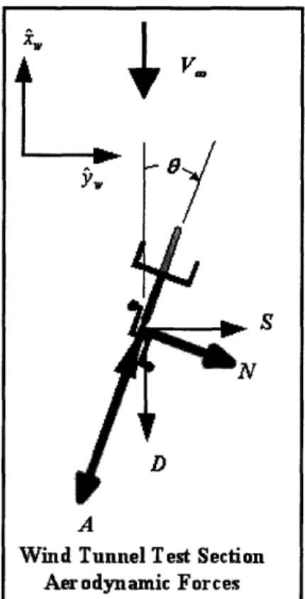
The coordinate system used in wind tunnel tests is shown in Figure 1. The wind axes are defined as follows: x points into the wind, y points to the right while facing the wind, and z points down. Aerodynamic forces are aligned with these axes. The lift, L, acts

in the negative z direction, drag, D, acts in the negative x direction, and side force S, acts in the positive direction.

Figure 1: Coordinate system used in wind tunnel and aerodynamic forces acting on a rider (Blair).

2.2.1 Forces Acting On Rider

The forces are summed to show that the total force acting on the bike/rider due to wind is

-=- A A A

Fw = -Doto xx+ Stot y, W- Lto Z(1

V.3

A

Wind Tunnel Test Section

Aerodynamic Forces

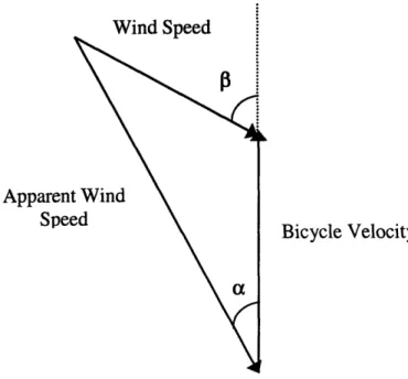
The apparent wind speed, which is the velocity the wind in the tunnel will be traveling at, can be calculated using simple geometry. Figure 2 shows a diagram of the relationship among the bicycle velocity, wind speed, and apparent wind speed.

Apparenl Spei

Bicycle Velocity

Figure 2: Correlation between rider speed, apparent wind speed and angle, and wind speed.

2.3 Wind

In real world conditions, wind speed varies in speed and incident angle on a daily basis. It is important to simulate these conditions as accurately as possibly in wind tunnel testing. A Weibull distribution is a continuous probability distribution and is commonly used to describe real life data; a mathematical model of wind was created using a Weibull distribution with a shape coefficient of 2. The model showed that the average deviation of incident wind is about 14'.

The yaw angles used in wind tunnel tests should be guided by the mathematical wind model in order to reflect real world racing conditions. Oftentimes larger yaw angles

are used by manufacturers to emphasize the benefit of their aerodynamic product in larger crosswinds, when in actuality the real world conditions show that, on average, wind hits a rider at angles less than fifteen degrees.

2.4 Current Protocol

The test is conducted in a constant wind tunnel velocity that best reflects the apparent wind velocity that the rider would experience. Several factors influence this, but it is common that the tunnel runs at 30 mph to mimic the speed of a professional rider. In order to measure drag, the test subject is attached to a load cell in the wind tunnel. The test may be performed in head-on wind only, or performed through a sweep of yaw angles, depending on the purpose of the test.

3. Test Overview 3.1 Helmets

Ten aero helmets were acquired for this test. These ten helmets include the helmets most popular in the world of professional cycling. The other helmet tested was a standard road helmet. The road helmet was used in the test in order to compare the results from aero helmets to the results from the standard road helmet.

3.1.1 Helmet Acquisition

In order to run the most comprehensive helmet study to date, several key helmet manufacturers were contacted to submit their aero helmets for testing. These critical manufacturers submitted their helmets to the project, creating a very extensive helmet lineup for testing. The helmets tested include the most popular aero road helmets in current racing. Note that the helmets that have a face shield attachment were tested with and without the shield.

In order to keep the individual manufacturer's data private, the helmets were randomly assigned a variable. In the thesis the helmets are referred to by their designated variable.

3.1.2 Control Helmet

A standard road cycling helmet was used as the control in this experiment. The testing could have been conducted with a helmet-less head as the control; however, this method of testing would not demonstrate the benefit that an aerodynamic helmet can provide over a regular road helmet. By using a road helmet as a comparative tool, the test provides a quantified difference between aero and road helmets.

3.2 Wind Tunnel Conditions

The wind tunnel will be set up to most accurately mimic a professional rider; the wind tunnel speed is set to 30 mph, which is equal to 13.4 m/s. The helmets will be

brought through a sweep of yaw angles from 00 to 150, in increments of 5". This sweep

reflects relevant racing conditions for a professional rider. 3.3 Helmet Mannequin

As discussed earlier, wind tunnel tests provide a large amount of control in athlete testing. However, athletes themselves bring another source of error to the data sets

because of human error. Though professionals may come very close to replicating their racing position time after time, there is still a slight discrepancy each time they reposition themselves. This uncertainty is avoided by using a stationary mannequin.

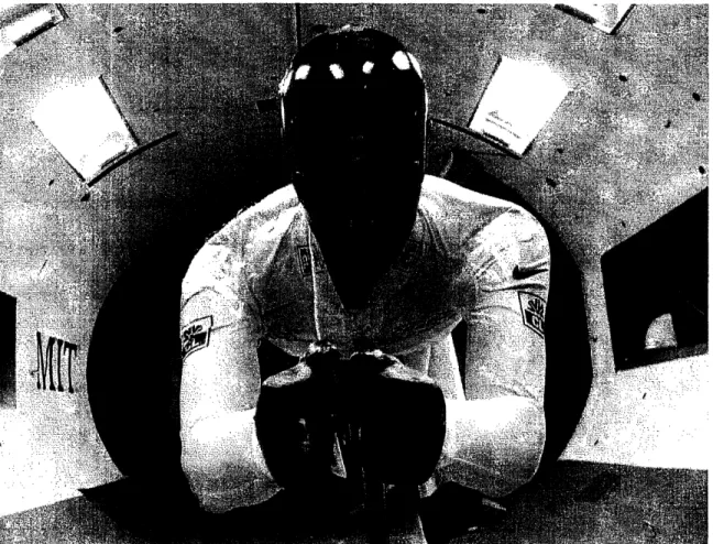
In these helmet tests, an upper body mannequin called Uri is used. Uri is bent forward at the waist and has his hands in front of him, as though he is on his aero bars.

He simulates a rider in the time trial position. The following figure shows the mannequin set up in the time trial position.

Figure 3: Picture of Uri the mannequin set up in the wind tunnel. He is in the aero position with his hands in front of him as though he were riding dropped down on aero bars.

3.4 Helmet Positions

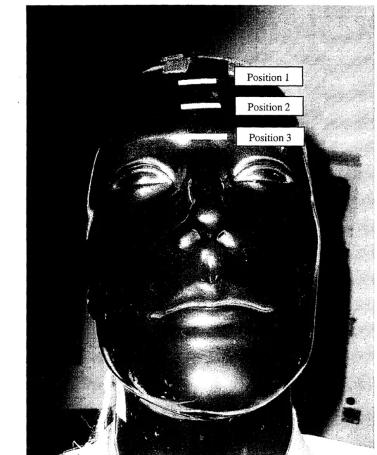
The helmets are tested in three different positions - placed very close to the back with the tip almost touching, placed slightly away from the back, and placed with the tip straight up. These positions represent relevant riding conditions (Fig 4, Fig 5). Position 1, with the tip very close to the back, represents what is believed to be the most

aerodynamic position for a rider. This is the way that most professionals race during time trials. The second position is with the tip slightly away from the back; this position replicates a rider moving away from the "ideal" position, due to fatigue or other factors.

The third and final position is with the tip straight in the air, which riders sometimes assume during a hill or mountain climb.

Safety is a critical factor in determining the validity of each helmet position. First and foremost, a helmet must provide a protective shell for the head. When placing the helmets on the head for testing, the researchers used the eyebrows as a reference line. The eyebrows serve as the line for position 2; position 1 was a measurable distance away from the eyebrows on the forehead. The placement for position 3 requires that the helmet is tipped straight up; however, because the neck of the mannequin is not a degree of freedom, the helmet is placed so that its brim touches the bridge of the nose.

These placement tactics ensure that the helmets meet their safety specifications. Figure 4 shows exactly where the helmets were placed on the head of the mannequin.

Figure 4: Picture of mannequin shows the reference lines on the forehead (in white) used in

positioning the helmet in order to model racing positions 1, 2, and 3.

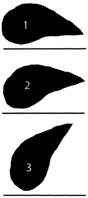
When the brim of the helmet is moved to different positions on the forehead, the back tail also moves. The following figure illustrates where the tail of the helmet is in relation to horizontal in each position.

Figure 5: Sketch of tail position in each of the helmet positions. The horizontal lines are reference lines.

4. Testing

The balance system used in the wind tunnel is a 6 component pyramidal balance and consists of a mechanical beam for the yawing moment system and a resistance strain gauge for the side force system ("WBWT"). Appendix A contains a table showing the

range and accuracies of the balance. The mannequin is mounted on the load cell for testing.

4.1 Test Sets

The test set collects data for 30 seconds. During this time, the software is

collecting data at 1000 Hz, recording tunnel wind speed, atmospheric conditions, and side force. A test sampling of 30 seconds provides enough data points to give confidence in the standard deviations and the error analysis.

4.2 Testing Procedure

A data set was recorded for each helmet at four different yaw angles with three

different helmet positions at each yaw angle, yielding twelve data sets for each helmet. The helmets that have visors were tested both with and without the visor.

All the helmets were tested in each position at each yaw angle before the table was moved to the next yaw position. Before moving to each yaw angle, the table was turned back to 00 and then moved to the desired position; this limited the possibility of propagating error through the test set by turning the table. Appendix B contains the procedure.

5. Results

This section includes the results from the twelve different data sets: three helmet positions at each of four different yaw angles. Section 5.1 goes through the results from head-on wind. The results from 50, 10', and 150 yaw are found in sections 5.2, 5.3, and 5.4, respectively. Complete helmet rankings can be found in appendices C-F. The standard deviations of each helmet test, as well as the 95% confidence intervals, are located in appendices H-J.

5.1 Head-on Wind

(00

Yaw)

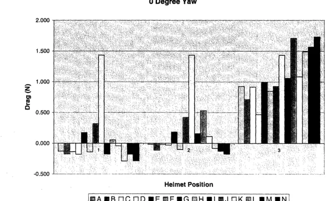
The drag results for the three different helmet positions in head-on wind are

shown in figure 6.

1.500

Figure 6: Drag values for each helmet in each of the three positions; the drag values shown are for the helmet itself. Note that helmet H is the control.

5.1.1 Helmet Position 1

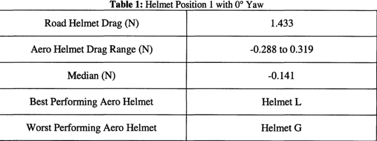
In helmet position 1, the best performing helmet had a drag value of -0.288 N. The worst performing helmet had a drag value of 0.319 N. (Note that this is the drag value of the helmet by itself; drag associated with the mannequin was subtracted out from the final drag value leaving only the value of the helmet.) The control road helmet drag value was 1.433 N. The median drag value was -0.141 N. Table 1 summarizes these results.

Table 1: Helmet Position 1 with 00 Yaw

Road Helmet Drag (N) 1.433

Aero Helmet Drag Range (N) -0.288 to 0.319

Median (N) -0.141

Best Performing Aero Helmet Helmet L

Worst Performing Aero Helmet Helmet G

5.1.2 Helmet Position 2

In helmet position 2, the best performing helmet had a drag value of -0.175 N. The worst performing helmet had a drag value of 0.530 N. Table 2 summarizes these results.

Table 2: Helmet Position 2 with 00 Yaw

Aero Helmet Drag Range (N) -0.175 to 0.530

Median (N) -0.017

Best Performing Aero Helmet Helmet N

Worst Performing Aero Helmet Helmet J

5.1.3 Helmet Position 3

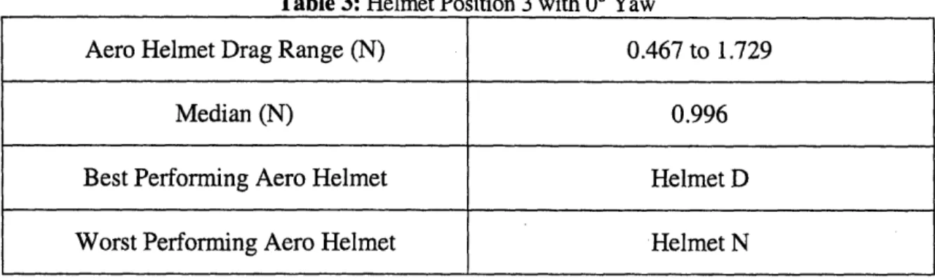
The drag value for the helmet with the lowest drag was 0.467 N, while the highest drag value measured for a helmet was 1.729 N. The median drag value was 0.996 N. Table 3 summarizes the key results from this data set.

Table 3: Helmet Position 3 with 00 Yaw

Aero Helmet Drag Range (N) 0.467 to 1.729

Median (N) 0.996

Best Performing Aero Helmet Helmet D

Worst Performing Aero Helmet Helmet N

5.2 Yaw of 50

Figure 7 highlights the average drag values for each helmet at a yaw angle of 50_in

each of the three positions that it was tested.

5 Degree Yaw

.1.8

H.

Figure 7: Drag values associated with each helmet at a yaw of 5' in each of the three helmet

positions. Note that helmet H is the control.

18 . . . .. . .... . 1 I -i i -i i

5.2.1 Helmet Position 1

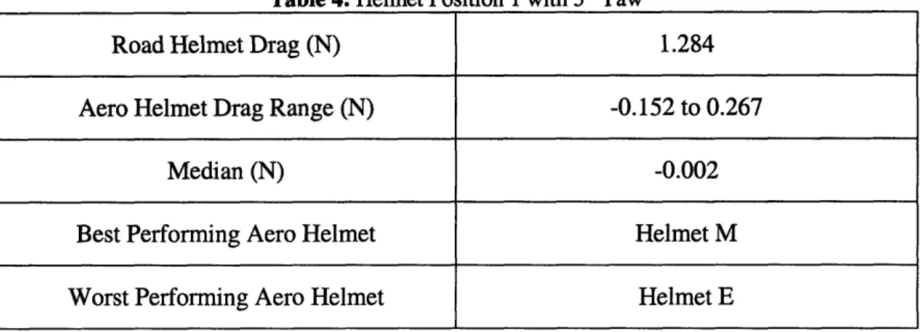
The drag value for the best performing helmet in position 1 at 5' yaw was -0.152 N, while the worst performing helmet had a drag value of 0.267 N. The median value for the helmet spread was -0.002. The control had a drag of 1.284 N. Table 4 highlights these results.

Table 4: Helmet Position 1 with 50 Yaw

Road Helmet Drag (N) 1.284

Aero Helmet Drag Range (N) -0.152 to 0.267

Median (N) -0.002

Best Performing Aero Helmet Helmet M

Worst Performing Aero Helmet Helmet E

5.2.2 Helmet Position 2

In helmet position 2, the drag value for the best performing helmet was 0.058 N, while the drag for the worst performing helmet was 0.581 N. The median value was 0.248 N. Table 5 summarizes these results.

Table 5: Helmet Position 2 with 50 Yaw

Aero Helmet Drag Range (N) 0.058 to 0.581

Median (N) 0.248

Best Performing Aero Helmet Helmet D

5.2.3 Helmet Position 3

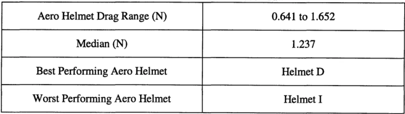
In position 3, the best performing helmet had a drag value of 0.641 N and the worst performing helmet had a value of 1.652 N. The median of this test set was 1.237 N. The following table highlights these results.

Table 6: Helmet Position 2 with 50 Yaw

Aero Helmet Drag Range (N) 0.641 to 1.652

Median (N) 1.237

Best Performing Aero Helmet Helmet D

Worst Performing Aero Helmet Helmet I

5.3 Yaw of 10O

The helmets were tested in the three positions at a yaw angle of 10'. Figure 8 shows how each helmet performed in each position.

10 Degree Yaw 2.000 I- ::·:: I I,··· 1.500 Z 1.000 0.500 0.000

4'

Figure 8: Drag values for each helmet in each position at a 100 yaw angle. Note that helmet H is

the control.

5.3.1 Helmet Position 1

In helmet position 1 at 100 yaw, the best performing helmet had a drag value of 0.002 N and the worst had a value of 0.383 N. The median value was 0.174 N. The control road helmet had a drag value of 1.422 N. Table 7 summarizes these results.

Table 7: Helmet Position 1 with 10' Yaw

Road Helmet Drag (N) 1.422

Aero Helmet Drag Range (N) 0.002 to 0.383

Median (N) 0.174

Best Performing Aero Helmet Helmet B

5.3.2 Helmet Position 2

The worst performing helmet in position 2 at 100 yaw had a drag value of 0.623 N while the best performing helmet had a drag value of 0.001 N. The median value was

0.174 N. The following table shows these results.

Table 8: Helmet Position 2 with 100 Yaw

Aero Helmet Drag Range (N) 0.001 to 0.623

Median (N) 0.174

Best Performing Aero Helmet Helmet B

Worst Performing Aero Helmet Helmet G

5.3.3 Helmet Position 3

In position 3, the best performing helmet had a drag value of 0.257 N. The worst performing helmet had a drag value of 1.950 N. The median value for this set was 1.125

N. Table 9 gives these results.

Table 9: Helmet Position 3 with 100 Yaw

Aero Helmet Drag Range (N) 0.257 to 1.950

Median (N) 1.125

Best Performing Aero Helmet Helmet B

Worst Performing Aero Helmet Helmet K

5.4 Yaw of 150

All the helmets were tested at a yaw angle of 15' in three different positions.

15 Degree Yaw 1.UUU 1.600 1.400 4 nn " :·~:::·-·--1·-;··~1-1--· i-~i~..,,.;:C;:· -·-···· · ·r:i-;:i .. !~: r:·~·· _i:· u:: ;,;···; _t: --..-...'.-- :n-;··-..:: : I·::· ··· I; - rli:::.i:...'..; i:.l':?;:i~-:l;'-,i::~;1 ·,···-··-;-I 1.200 1.000 0.800 0.600 0.400 0.200 U.UUU Helmet Position UA EB OC OD ME OF NG !JH MII WJ OK M L MM iN 1

Figure 9: Data from 150 yaw test. The helmets were all tested in three different helmet positions

on the head. Note that helmet H is the control.

5.4.1 Helmet Position 1

At a 15' yaw angle in position 1, the drag value for the best performing helmet was 0.006 N; the drag value for the worst performing helmet was 0.329 N. The median value was 0.113 N and the control helmet had a drag value of 1.097 N. Table 10 summarizes these results.

Table 10: Helmet Position 1 with 15' Yaw

Road Helmet Drag (N) 1.097

Aero Helmet Drag Range (N) 0.006 to 0.329

Median (N) 0.113

Best Performing Aero Helmet Helmet B

Worst Performing Aero Helmet Helmet E

·· 2.000 _{7777-t·:·- ·}

':· ~.i ?·:·::`I;_i': ·-·i,

5.4.2 Helmet Position 2

The worst performing helmet in position 2 at a 150 yaw angle had a drag value of 0.416 N while the best performing helmet had a drag value of 0.018 N. The median value was 0.118 N. These results can be seen in Table 10.

Table 10: Helmet Position 2 with 150 Yaw

Aero Helmet Drag Range (N) 0.018 to 0.416

Median (N) 0.118

Best Performing Aero Helmet Helmet L

Worst Performing Aero Helmet Helmet J

5.4.3 Helmet Position 3

In position 3 at a 15' yaw angle, the worst performing helmet had a drag value of 1.785 N. The best performing helmet in these conditions had a drag value of 0.423 N. The median value was 1.232 N. Table 11 shows these results.

Table 11: Helmet Position 3 with 150 Yaw

Aero Helmet Drag Range (N) 0.423 to 1.785

Median (N) 1.232

Best Performing Aero Helmet Helmet B

Worst Performing Aero Helmet Helmet J

6. Discussion

Aerodynamic helmets do reduce a rider's drag when compared to a standard road helmet. Even the worst performing helmets in testing provide drag reduction from the

control. It is interesting to note that even though the range of drag values can be large for the helmet spread, the aero helmets still prove to have less drag than the road helmet. 6.1 Drag Reduction and Power Savings

An aero helmet lowers drag. Because drag is the majority of what a rider must overcome in order to move, a reduction in drag could equate to a power "savings" for that rider. To clarify, a rider would need less power in order to overcome drag. Sections 6.1.1 and 6.1.2 will show the power savings for two types of riders: professional racers and amateur cyclists. In order to analyze the relative power savings and drag reduction, two assumptions had to be made. The amount of drag that each type of rider typically has (including a road helmet) and the average power output over 40 km. It was estimated that an amateur cyclist has roughly 27 N of drag and has a power output of 225 Watts. The professional cyclist has 22 N of drag and a power output of 450 Watts. (Martin et al)

The percent drag reduction is given by

RoadHelmetDrag - AeroHelmetDrag x100, (2)

TotalDrag

where the road helmet drag is given by the drag value for the control, the aero helmet drag is the drag associated with a particular aero helmet, and the total drag is the drag value for the rider and all associated equipment. In the following cases, the total drag is either 27 N or 22 N, depending on whether it is an amateur or professional rider,

respectively.

The amount of power savings is determined by multiplying the percent drag reduction by the power output of a rider. The following equation shows how the power savings are calculated.

6.1.1 Professional Cyclist

A typical professional cyclist has close to five pounds of drag (including a

standard road helmet), which is 22 N, and outputs an average of 450 Watts during a time trial. This information can be used to compute exactly how much a pro would benefit from the use of an aero helmet. Tables 12, 13, 14, and 15 show the percent drag reduction and the power savings to pro riders if they switched from a road helmet to an aero helmet at 00, 50, 100, and 150 yaw angles, respectively. It is interesting to note that even the worst performing aero helmet offers a benefit to the rider.

Table 12: Drag Reduction and Power Savings for a Professional Rider at 00 Yaw

Pro: 22 N Drag and Best Helmet _{Median Helmet Worst Helmet}

450 Watts Power

% Drag Reduction 7.8% 7.2% 5.1%

Power Savings 35.2 Watts 32.2 Watts 22.8 Watts

Table 13: Drag Reduction and Power Savings for a Professional Rider at 50 Yaw

Pro: 22 N Drag and Best Helmet _{Median Helmet Worst Helmet} 450 Watts Power

% Drag Reduction 6.5% 5.8% 4.6%

Power Savings 29.3 Watts 26.3 Watts 20.8 Watts

Table 14: Drag Reduction and Power Savings for a Professional Rider at 10' Yaw

Pro: 22 N Drag and Best Helmet _{Median Helmet}

Worst Helmet

450 Watts Power

% Drag Reduction 6.5% 5.7% 4.7%

Table 15: Drag Reduction and Power Savings for a Professional Rider at 150 Yaw

Pro: 22 NDrag and Best Helmet _{Median Helmet Worst Helmet}

450 Watts Power

% Drag Reduction 5.0% 4.5% 3.5%

Power Savings 22.3 Watts 20.1 Watts 15.7 Watts

6.1.2 Amateur Cyclist

An amateur rider will also see power savings and drag reduction if they switch to an aerodynamic helmet. It is harder to define the "typical" amateur athlete than it is to define the "typical" professional in terms of power output and amount of drag associated with the riding position and equipment. For the purpose of this analysis, it is assumed that the average amateur athlete has roughly 6 pounds of drag, which is about 27 N, and can output an average of 225 Watts of power during a time trial.

Through the sweep of yaw angles, the median helmet saw an average of 4.7% drag reduction and a power savings of 8.3 Watts with an aero helmet. Tables 16, 17, 18, and 19 show the percent drag reduction and the power savings an amateur would see at 0o, 50, 100, and 150 yaw angles with an aero helmet versus a road helmet.

Table 16: Drag Reduction and Power Savings for an Amateur Rider at 00 Yaw

Amateur: 27 N Drag Best Helmet _{Median Helmet Worst Helmet} and 225 Watts Power

% Drag Reduction 6.4% 5.8% 4.1%

Table 17: Drag Reduction and Power Savings for an Amateur Rider at 50 Yaw

Amateur: 27 N Drag Best Helmet Median Helmet _{Worst Helmet}

and 225 Watts Power

% Drag Reduction 5.3% 4.8% 3.8%

Power Savings 12.0 Watts 10.7 Watts 8.5 Watts

Table 18: Drag Reduction and Power Savings for an Amateur Rider at 100 Yaw

Amateur: 27 N Drag Best Helmet Median Helmet _{Worst Helmet}

and 225 Watts Power

% Drag Reduction 5.3% 4.6% 3.8%

Power Savings 11.8 Watts 10.4 Watts 8.7 Watts

Table 19: Drag Reduction and Power Savings for an Amateur Rider at 150 Yaw

Amateur: 27 N Drag Best Helmet _{Median Helmet Worst Helmet}

and 225 Watts Power

% Drag Reduction 4.0% 3.6% 2.8%

Power Savings 9.1 Watts 8.2 Watts 6.4 Watts

7. Conclusion

Ten aerodynamic helmets were tested side by side in an extensive wind tunnel study. These helmets were compared to a standard road helmet and it was found that aerodynamic helmets provide drag reduction versus the road helmet. While there may be a significant range of performance between the helmet spread, all of the helmets offered a benefit over a road helmet.

By wearing an aero helmet, a rider can save a considerable amount of power and

can also substantially reduce his overall drag. This study quantified the benefit of wearing an aero helmet and gives important data that can be compared to the rest of cycling

equipment. Also, the test protocol used in this study can be applied to any future helmet tests.

7.1 Recommendations

Ideally, more extensive research will be conducted on helmets. The research could be expanded in order to better understand the theory behind helmets and their sources of drag and drag reduction. This type of testing would entail flow visualizations, pressure measurements, and could lead to the discovery of the most ideal helmet shape.

A study in which the specific helmet names can be published would be beneficial. This would allow for the researcher to theorize what particular helmet shapes work best in drag reduction and why this happens. It would also allow for better understanding of the theory behind helmet drag and could be used to make athletes faster.

Works Cited

Blair, Kim. "Cycling Aerodynamics." Serotta International Cycling Institute, SICI Cycling Science Symposium and Expo. Hotel Boulderado, Boulder, CO. 23 January, 2007.

"fluid mechanics." Encyclopedia Britannica. 2007. Encyclopedia Britannica Online. 8 May 2007. Online Academic Edition. <http://www.search.eb.com/eb/article-77496>.

Martin, James C., Douglas L. Milliken, John E. Cobb, Kevin L. McFadden, and Andrew R. Coggan. "Validation of a Mathematical Model for Road Cycling Power." Journal of Applied Biomechanics. 14 (1998): 276-291

"WBWT Information for Industry." MIT's Wright Brothers Wind Tunnel. July 2002. 10 May 2007 < http://web.mit.edu/aeroastro/www/labs/WBWT/>

Appendix A. Characteristics of the Mechanical Balance

(From the MIT's Wright Brothers Wind Tunnel Information for Industry Article - July 2002)

CHARACTERISTICS OF THE MECHANICAL BALANCE

Model Mounts

Standard 3 Strut -Two forward plus a tall strut for angle of attack control. Available spacings:

Front trunnions -28 to 42 inches (reducible to 4 1/2 to 11 1/2 with special slant trunnions)

Rear strut -20 to 36 inches

Single central strut -a plus aft tail strut for angle of attack control

Balance type -6 component pyramidal Angle of attack Angle of Yaw Lift Drag Side force Pitching moment Rolling moment Yawing moment Range -300 to +300 -200 to +200 0 to 3000 lb 0 to 600 lb -300 to +300 lb -350 to +350 lb -350 to +350 ft lb -300 to +300 ft lb Accuracies (2) 0.10 0.10 0.5 lb 0.03 lb 0.1 lb 0.2 ft lb 0.2 ft lb 0.2 ft lb Sting balances are available

(1) For 30-inch spacing between front and rear support

Appendix B. Procedure

1. Place helmet A on mannequin in helmet position 1. 2. Run a 30 second test set.

3. Record drag values and standard deviations. 4. Move helmet A into position 2.

5. Repeat steps 4 and 5.

6. Move helmet A into position 3. 7. Repeat steps 4 and 5.

8. Remove helmet A from mannequin.

9. Run 30 second test set on mannequin alone.

10. Repeat steps 1 through 11 on helmets B through N. 11. Yaw table to 50 and do steps 1-12.

12. Yaw table to 00.

13. Yaw table to 100 and do steps 1-12. 14. Yaw table to 00.

Appendix C. Ranking of Helmets at 00 Yaw

Helmet Position 1 Helmet Position 3

Helmet L N D M I B F C A K J E G H 0 Degree Drag (N) -0.288 -0.286 -0.179 -0.176 -0.175 -0.174 -0.141 -0.136 -0.129 -0.042 0.055 0.175 0.319 1.433 Rank 1 2 3 4 5 6 7 8 9 10 Helmet D B F C A G E I K H L M J N 0 Degree Drag (N) 0.467 0.713 0.847 0.914 0.926 0.927 0.996 1.060 1.083 1.433 1.488 1.565 1.708 1.729 Helmet Position 2

Rank Helmet 0 Degree Drag (N)

1 N -0.175 2 M -0.127 3 B -0.112 4 F -0.100 5 L -0.082 6 D -0.029 7 C -0.017 8 A -0.017 9 K 0.112 10 I 0.158 11 E 0.183 12 G 0.422 13 J 0.530 14 H 1.433 Rank 1 2 3 4 5 6 7 8 9 10 11 12 13 14

Appendix D. Ranking of Helmets at 50 Yaw Helmet Position 1 Rank 1 2 3 4 5 6 7 8 9 10 11 12 13 14 Helmet M L N D B F K C A I J G E H Helmet Position 3 5 Degree Drag (N) -0.152 -0.138 -0.137 -0.121 -0.042 -0.008 -0.002 0.065 0.066 0.130 0.192 0.262 0.267 1.284 Rank 1 2 3 4 5 6 7 8 9 10 11 12 13 14 Helmet D B C F G A L E H K M N J I 5 Degree Drag (N) 0.641 0.649 0.731 0.900 1.003 1.218 1.237 1.241 1.284 1.464 1.558 1.627 1.648 1.652 Helmet Position 2

Rank Helmet 5 Degree Drag (N)

1 D 0.058 2 B 0.098 3 M 0.109 4 N 0.123 5 F 0.125 6 C 0.190 7 A 0.248 8 K 0.288 9 L 0.290 10 E 0.392 11 I 0.539 12 J 0.544 13 G 0.581 14 H 1.284

Appendix E. Ranking of Helmets at 100 Yaw Helmet Position 1 Rank 1 2 3 4 5 6 7 8 9 10 11 12 13 14 Helmet B I A F M C D N K E L J G H Helmet Position 3 10 Degree Drag

(N)

(N)

Appendix F. Ranking of Helmets at 150 Yaw

Helmet Position 1 Helmet Position 3

15 Degree Drag

(N)

(N)

(N)

Appendix G. Standard Deviation and 95% Confidence Intervals for 00 Yaw Helmet Helmet Position

A 1 2 3 B 1 2 3 C 1 2 3 D 1 2 3 E 1 0 Degree Drag (N) -0.129 -0.017 0.926 -0.174 -0.112 0.713 -0.136 -0.017 0.914 -0.179 -0.029 0.467 0.175 0.183 0.996 -0.141 -0.100 0.847 0.319 0.422 0.927 1.433 0.055 0.530 1.708 -0.042 0.112 1.083 -0.175 0.158 1.060 -0.288 -0.082 1.488 -0.176 -0.127 1.565 -0.286 -0.175 1.729 0 Std Dev (N) 0.062 0.102 0.089 0.067 0.062 0.085 0.071 0.076 0.080 0.053 0.071 0.058 0.067 0.058 0.089 0.053 0.116 0.129 0.062 0.093 0.093 0.067 0.067 0.044 0.062 0.076 0.071 0.053 0.111 0.080 0.071 0.053 0.138 0.125 0 107 0.076 0.093 0.067 0.076 0.080 0 95% Confidence 0.045 0.074 0.065 0.049 0.045 0.062 0.052 0.056 0.058 0.039 0.052 0.042 0.049 0.042 0.065 0.039 0.085 0.094 0.045 0.068 0.068 0.049 0.049 0.032 0.045 0.055 0.052 0.039 0.081 0.058 0.052 0.039 0.101 0.091 0.078 0.056 0.068 0.049 0.056 0.058

Appendix H. Standard Deviation and 95% Confidence Intervals for 50 Yaw Helmet A B C D E F G H I Helmet Position 1 2 3 1 2 3 1 2 3 1 2 3 1 2 3 1 2 3 1 2 3 1 1 2 3 5 Degree Drag (N) 0.066 0.248 1.218 -0.042 0.098 0.649 0.065 0.190 0.731 -0.121 0.058 0.641 0.267 0.392 1.241 -0.008 0.125 0.900 0.262 0.581 1.003 1.284 0.192 0.544 1.648 -0.002 0.288 1.464 0.130 0.539 1.652 -0.138 0.290 1.237 -0.152 0.109 1.558 -0.137 0.123 1.627 5 Std Dev (N) 0.111 0.085 0.098 0.062 0.089 1.704 0.098 0.107 0.071 0.080 0.076 0.116 0.089 0.080 0.107 0.062 0.085 0.085 0.102 0.076 0.102 0.067 0.089 0.093 0.111 0.085 0.080 0.125 0.089 0.076 0.080 0.093 0.085 0.102 0.076 0.089 0.116 0.098 0.102 0.085 5 95% Confidence 0.081 0.062 0.071 0.045 0.065 1.244 0.071 0.078 0.052 0.058 0.055 0.084 0.065 0.058 0.078 0.045 0.062 0.062 0.075 0.055 0.075 0.049 0.065 0.068 0.081 0.062 0.058 0.091 0.065 0.055 0.058 0.068 0.062 0.075 0.055 0.065 0.084 0.071 0.075 0.062

Appendix I. Standard Deviation and 95% Confidence Intervals for 100 Yaw Helmet Helmet Position

A 1 2 3 B 1 2 3 C 1 2 3 D 1 2 3 E 1 2 3 F 1 2 3 G 1 2 3 H 1 I 1 2 3 J 1 2 3 K 1 2 3 L 1 2 3 M 1 2 3 N 1 2 3 10 Degree Drag (N) 0.030 0.140 1.125 0.002 0.001 0.257 0.064 0.153 0.654 0.174 0.186 0.588 0.244 0.426 1.134 0.059 0.090 0.473 0.383 0.623 1.015 1.422 0.338 0.421 1.663 0.230 0.578 1.950 0.026 0.368 1.436 0.264 0.017 1.061 0.059 0.117 1.718 0.194 0.174 1.633 10 Std Dev (N) 0.067 0.093 0.107 0.080 0.080 0.076 0.067 0.085 0.067 0.067 0.076 0.089 0.071 0.076 0.076 0.071 0.067 0.076 0.067 0.085 0.089 0.080 0.067 0.058 0.085 0.076 0.080 0.116 0.080 0.098 0.102 0.062 0.067 0.093 0.053 0.071 0.093 0.067 0.071 0.089 10 95% Confidence 0.049 0.068 0.078 0.058 0.058 0.055 0.049 0.062 0.049 0.049 0.055 0.065 0.052 0.055 0.055 0.052 0.049 0.055 0.049 0.062 0.065 0.058 0.049 0.042 0.062 0.055 0.058 0.084 0.058 0.071 0.075 0.045 0.049 0.068 0.039 0.052 0.068 0.049 0.052 0.065

Appendix J. Standard Deviation and 95% Confidence Intervals for 150 Yaw Helmet Helmet Position

A 1 2 3 B 1 15 Degree Drag (N) 0.040 0.093 1.269 0.006 0.066 0.423 0.111 0.267 0.451 0.208 0.203 0.538 0.329 0.245 1.002 0.166 0.020 0.482 0.246 0.317 1.041 1.097 0.274 0.416 1.785 0.069 0.171 1.232 0.092 0.118 1.631 0.113 0.018 1.237 0.080 0.070 1.588 0.314 0.038 1.423 15 Std Dev (N) 0.076 0.062 0.258 0.049 0.062 0.058 0.071 0.062 0.071 0.058 0.062 0.089 0.049 0.071 0.071 0.058 0.076 0.080 0.076 0.076 0.076 0.071 0.062 0.085 0.085 0.053 0.076 0.062 0.058 0.053 0.071 0.067 0.067 0.085 0.044 0.067 0.053 0.071 0.085 0.076 15 95% Confidence 0.055 0.045 0.188 0.036 0.045 0.042 0.052 0.045 0.052 0.042 0.045 0.065 0.036 0.052 0.052 0.042 0.055 0.058 0.055 0.055 0.055 0.052 0.045 0.062 0.062 0.039 0.055 0.045 0.042 0.039 0.052 0.049 0.049 0.062 0.032 0.049 0.039 0.052 0.062 0.055