ARDA: Automatic Relational Data Augmentation
for Machine Learning
by
Nadiia Chepurko
Submitted to the Department of Electrical Engineering and Computer
Science
in partial fulfillment of the requirements for the degree of
Master of Science in Computer Science and Engineering
at the
MASSACHUSETTS INSTITUTE OF TECHNOLOGY
February 2020
@
Massachusetts Institute of Technology 2020. All rights reserved.
Signature redacted
A u th or ...
Department of Electrical Engineering
omputer Science
(January
30, 2020
Signature redacted
C ertified by ...
... ...
David R. Karger
Professor of Electrical Engineering and Computer Science
Thesis Supervisor
Accepted by
...
Signature redacted....
is
mWE
/
Ie4
A.
Kolodziejski
Professor of Electrical Engineering and Computer Science
MR 13
2020
Chair, Department Committee on Graduate Students
ARDA: Automatic Relational Data Augmentation for
Machine Learning
by
Nadiia Chepurko
Submitted to the Department of Electrical Engineering and Computer Science on January 30, 2020, in partial fulfillment of the
requirements for the degree of
Master of Science in Computer Science and Engineering
Abstract
This thesis is motivated by two major trends in data science: easy access to tremen-dous amounts of unstructured data and the effectiveness of Machine Learning (ML) in data driven applications. As a result, there is a growing need to integrate ML models and data curation into a homogeneous system such that the model informs the choice and extent of data curation. The bottleneck in designing such a system is to efficiently discern what additional information would result in improving the generalization of the ML models.
We design an end-to-end system that takes as input a data set, a ML model and access to unstructured data, and outputs an augmented data set such that training the model on this dataset results in better generalization error. Our system has two distinct components: 1) a framework to search and join unstructured data with the input data, based on various attributes of the input and 2) an efficient feature selection algorithm that prunes our noisy or irrelevant features from the resulting join. We perform an extensive empirical evaluation of system and benchmark our feature selection algorithm with existing state-of-the-art algorithms on numerous real-world datasets.
Thesis Supervisor: David R. Karger
Acknowledgments
First and foremost, I would like to thank my advisor, David Karger, without whose unwavering support this thesis would not be possible. I would also like to thank Tim Kraska for outlining the goals of the project and providing valuable insights during crucial stages. In addition, I am grateful to my collaborators Raul Castro Fernandez, Ryan Marcus and Emmanuel Zgraggen.
Contents
1 Introduction 13 1.1 Introduction . . . . 13 1.2 Related Work . . . . 15 1.3 Problem Description . . . . 18 2 Data Augmentation 21 2.1 Augmentation workflow . . . . 21 2.1.1 Coreset Constructions . . . . 24 2.2 Joins . . . . 27 2.2.1 Join type . . . . 27 2.2.2 Key Matches . . . . 28 2.2.3 Join cardinality . . . . 30 2.2.4 Imputation . . . . 30 3 Feature Selection 33 3.1 Overview of Feature Selection . . . . 333.2 Random Injection Based Feature Selection . . . . 36
3.2.1 Random Feature Injection . . . . 38
3.2.2 Ranking Ensembles . . . . 39
3.2.3 Aggregate Ranking . . . . 41
3.2.4 Putting it together. . . . . 41
4 Experiments
47
4.1
M icro Benchmarks ...
47
4.2 Coreset Comparison
. . . .
49
4.3 Experimental Evaluation of ARDA . . . .
51
List of Figures
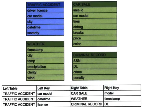
1-1 Example Schema: Initially a user has a base table TRAFFICACCIDENT and she finds a pool of joinable tables to see if some of them can help improve prediction error for severity of a traffic accident. . . . . 19
2-1 The A RDA . . . . 22
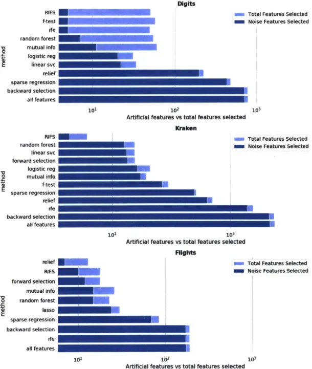
4-1 Comparison of the running time for each feature selection algorithm with the improvement in prediction accuracy achieved over the base table (no augmentation). . . . . 49 4-2 Micro Benchmark for Feature Selection Algorithms on Digits, Kraken
and Flights data sets. The original data sets are appended with 1000 x artificial, noisy features (as described above). The x-axis represents number of features, the y-axis denotes the algorithm and the plot com-pares the true features extracted vs the artificial features extracted. . 50
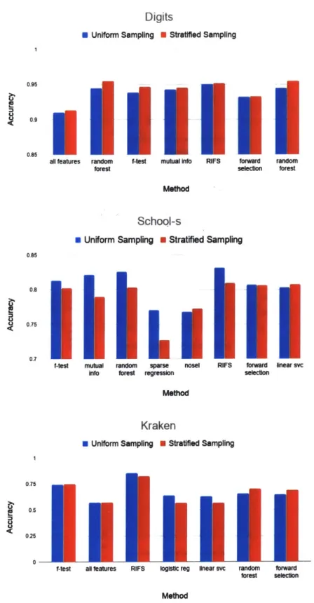
4-3 Coreset comparison using various feature selection algorithm on School, Digits and Kraken data sets. The coresets are construction via Uniform or Stratified sampling 1000 training samples. The x-axis denotes the feature selection algorithms and the y-axis denotes the corresponding prediction accuracy. . . . . 53
4-4 Comparison of the running time for each feature selection algorithm with the improvement in prediction accuracy achieved over the base table (no augmentation). . . . . 54
List of Tables
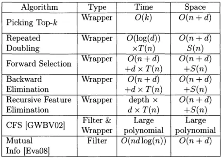
3.1 Comparison of popular subset selection algorithms, given a ranking of the features. We note that various learning models provide the rank-ing for these algorithms. T(n) denotes the time evaluate the learnrank-ing algorithm and S(n) is the corresponding space used. . . . . 34
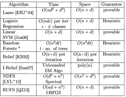
3.2 Comparison of popular learning models for feature selection. . . . . . 35
4.1 We compare the performance of joining one table at a time vs join-ing at most |SI features at a time (ISI is the size of a coreset). The first column denotes the multiplicative speedup factor and the second column denotes increase in accuracy w.r.t. full materialization. . . . 52
4.2 We compare the performance of joining all tables at once (full mate-rialization) vs joining at most |SI features at a time (ISI is the size of a coreset). The first column denotes the multiplicative speedup fac-tor and the second column denotes increase in accuracy w.r.t. full m aterialization. . . . . 52
Chapter 1
Introduction
1.1
Introduction
Today we have the access to tremendous amounts of data on the web. Google Dataset Search provides a simple interface to mine data from various sources. Governments, academic institutions and companies are making their data sets publicly available. This, combined with the astonishingly increasing use of machine learning (ML) in data driven applications has led to a growing interest in integrating ML and data curation/processing. However, existing ML toolkits and frameworks assume that the data is stored in a single table on a single machine. On the contrary, most of the data is stored across the web, in an unstructured form across multiple tables connected by key-foreign key dependencies (KFKDs).
Since the success of modern ML techniques, such as Deep Learning, is contingent on larger training sets and more features, analysts spend a majority of their time finding relevant data to answer the questions at hand than trying various algorithmic solutions and analyzing the results. The need for data and feature discovery discov-ery has therefore opened the door for a new research area that tries to utilize this additional features for improving prediction tasks. Data Enrichment is one such area that only recently defined itself as a response to a need of improved ML predictions
by agglomerating data from external knowledge sources. This paper focuses on the
for a ML task by finding and adding relevant features from multiple heterogeneous sources.
For instance, consider the critical task of predicting the taxi demand for a given day. Accurate prediction is important for taxi companies in order to dispatch the right amount of cars for cost optimization. The company gathers the history of all the taxi trips over a period of time, as well as statistics of the trip like start time, end time, distance covered, route taken and so on. However, given information might not be enough for accurate predictions of the future demand, even for the "perfect" learning model. In this scenario the remaining solution is to search for external knowledge that we can augment in original dataset to improve the prediction. An example of such knowledge source is a weather dataset that is implicitly connected with taxi data through KFKD relationship on time series columns. Weather datasets are readily available online and can be successfully incorporated using the join procedure.
While in this example it wasn't hard for us to infer the strong correlation be-tween taxi demand and weather conditions, automating such inference for different tasks over massive, unstructured data is extremely challenging. Knowledge Discovery and Data Mining study algorithms to extract a semantic understanding from large amounts of unstructured data. However, for a given predictive task, the space of possible augmentations grows exponentially in the size of the data and a semantic understanding does not provide new features to augment our initial dataset. Explor-ing each possibility quickly becomes computationally infeasible. Further, each aug-mentation adds a computational overhead in terms of data cleaning, pre-processing and performing a join.
Since most of the open source datasets have only meager unstructured description, or no description at all, we cannot rely on semantic relationships between datasets to infer their logical connections. It is also possible that semantic relationships do not imply feature-target correlation. For example, taxi and weather has small semantic correlation, but very strong predictive correlation for the aforementioned learning task. Therefore, apriori, we do not know what features are useful in the prediction task and what features are coming from spurious irrelevant datasets.
Further, agnostically adding all joinable features at once results in an extremely noisy training set. Existing ML models are brittle to noise and thus generalize poorly in such a setting. In particular, massive noise can wash out existing signal and prediction performance may drop below the baseline score altogether. Therefore, we require a system that automatically and efficiently discovers relevant features to extract from a large set of potentially joinable tables, such that the augmented data set improves the generalization error of the ML model. Our main contribution is to design an end-to-end system that incorporates data formatting, sampling, joining, aggregation, imputation and feature selection (or pruning noise) such that the ML model obtains better performance on prediction tasks.
1.2
Related Work
While there has been extensive prior work on Data Mining, Knowledge Discovery, Data Augmentation and Feature Selection, we are not aware of previous work on feature discovery via database joins to improve performance of predication tasks. We provide a brief overview of this literature and indicate how it differs from our setup.
Data Mining and Knowledge Discovery. Knowledge Discovery (KD)
fo-cuses on extracting useful information from large data sets and aims at a semantic understanding of this data. The algorithms developed extract new concepts or con-cept relationships hidden in volumes of raw data. See [ME08] for a survey on KD and [KM06] for overview in the context of databases. Data Mining (DM) is the appli-cation of specific algorithms for the extraction of nuggets of knowledge, i.e., pertinent patterns, pattern correlations, estimation or rules, from data. These algorithms in-clude Clustering [Ber06], Regression and PCA [LL06]. In this vast literature, we focus on Data Discovery and Data Augmentation for finding related tables.
Data Discovery. Data Discovery systems deal with sharing datasets,
search-ing new datasets, and discoversearch-ing relationships withsearch-ing heterogeneous data pool. There have been several works that extract tables from the Web [BDE+15, BBC+14,
pages relying on positional information of visualized DOM element nodes in a browser. Cafarella et al. [CHK09] developed the WebTables system for web-scale table extrac-tion, implementing a mix of hand-written detectors and statistical classifiers, and Oc-topus
[YGCC12]
even try to identify additional information from online data sources. The Aurum system [FAK+18] helps find KFKDs between different sources of data. In addition to the above systems, there are many data portal platforms such as CKAN, Quandl, DataMarket, Kaggle etc. Work on data searching lakes includes but not lim-ited to [TSRC15,HKN+16b,HKN+16a,TSRC15,CFDM+17]. Recently Google release Google Dataset Search engine that helps finding datasets across different web portals in no time.Data Augmentation. Data Augmentation has three main techniques:
embed-ding augmentation, entity augmentation, and join augmentation. The goal of em-bedding augmentation is to learn document's low dimensional representations and be able to compare these representations to decide which documents have higher chance to describe a similar data under some notion of similarity. Some popular text em-beddings include Word2Vec [MSC+13], Doc2Vec [LM14], and Table2Vec [Den18] that let us convert an entire document into vector representation. Entity augmentation deals with finding and bringing additional data that describes the same entity. Oc-topus is a system that combines search, extraction, data cleaning and integration, and enables users to create new data sets from those found on the Web. InfoGather presents three core operations, namely entity augmentation by attribute name, entity augmentation by example and attribute discovery, that are useful for "information gathering" tasks. Augmentation using Joins is one of the most recent research areas within Data Augmentation. The motivating problem stems from the fact that ML systems let you to feed a single csv file with an assumption that this file contains all needed information for predictive tasks. Since most databases have normalized schemas and so facts are scattered across multiple tables one needs to perform joins before running ML models. In projects Hamlet/Hamlet++ and their corresponding papers [KNPZ16] and [SKZ17] authors study effects of KFKDs within normalized databases. They propose a set of decision rules to predict when it is safe to avoid
joins and reduce the processing time.
Data Generation. During join discovery, one almost certainly has to deal with
missing values. This process is referred to as data imputation and is a challenging problem for mixed datasets. The two main types of data generation include crowd-sourcing and synthetic data generation that if further divided into statistics-based methods and machine learning based methods. We refer the reader to the
follow-ing [MWYJO2,DVDHSM06,GBGB9,GLH15,PHW16,YWL+16,LG17,SPC+19] and
references therein. While data generation can help to fill in missing entries, the tech-niques developed here do not lend themselves well to data augmentation.
Robustness and Bias- Variance Tradeoff. A recent line of work on adversarial
learning also provides evidence to the challenging nature of selecting features in the presence of noise and unstructured data. A natural approach to feature augmentation would be to join all compatible tables and rely of the learning algorithm to ignore irrelevant features. However, this requires our learning models to be incredibly robust to noisy features.
Unfortunately, ML algorithms are highly sensitive to noisy, possibly adversarial
features [MMS+17, WK17, SZS+13, CW17, AEIK17]. Therefore, the challenge of
ef-ficiently finding relevant features to join with our base table, while simultaneously pruning out noise remains.
Given that the feature set plays a crucial role the in the predictive power of ML models, removing redundant and irrelevant features is crucial and has been extensively studied. The conventional wisdom in designing feature selection algorithms is to reduce both bias and variance of the model. Recall, bias accumulates when the model tries to generalize using erroneous assumptions in the training data and noisy features contribute to the variance [Dom99].
It is well known that the more sensitive the model is to the training data, the lower the bias in exchange for a higher variance'. Therefore, classifiers with limited data use feature selection to find an optimum point where they can actually estimate
1
See Wikipedia page on Bias-Variance Tradeoff https://en.wikipedia.org/wiki/ Bias&ilvariancetradeoff
the statistical distribution of fewer features (variance reduction) versus less accurate estimation of more features (bias reduction) [Fri97, KJ97]. However, our approach instead relies on finding as many relevant features as possible. While such an approach works in practice, classical theory suggests it should lead to over-fitting.
1.3
Problem Description
In this section, we describe the precise setup and problem statement we consider. Our system is given as input a base table with labelled data and the goal is to perform inference on this dataset. We assume the learning model is also specified and typically is computationally expensive to train. The models we train include Random Forests, Logistic Regression, Lasso and SVMs. We also assume we have access to a hold-out set where we can test the performance of our algorithms on fresh data to inform hyper-parameter search. We train the learning model on our base table and test it on the holdout set to obtain a baseline score.
Our goal then is to augment features to our base table such that we can obtain a non-trivial improvement on the prediction task. To this end, we assume we know the key on which we should attempt to join new tables with the base table. Here, we allow for both hard and soft joins. For instance, if the base key specifies time-series data, we automatically perform soft join using nearest neighbour approach or linear interpolation over backward/forward join. We note that for soft joins over non-time data our system needs explicit indication of a soft join (specified as * over the join key), otherwise standard exact-match join is performed.
In order to collect joinable datasets for our basetables described in Chapter 2 used the DataMart
/
Auctus 2 repository to search for datasets over the web. DataMart is a web crawler and search engine for datasets, specifically designed for join discovery. While DataMart provides multiple potential tables to join with, most of the aug-mented features are spurious since they are coming from datasets that have no useful information for the target learning task. The datasets are collected from numerous2
FIC ACCIDENT driver licence arc model city datetime severity rEATHERc timestamp city temp precipitation clarity wind CAR SALE sale id car model ires airbag breaks price
Left Table Left Key RIhtTable Right Key
TRAFFIC ACCIDENT car model CAR SALE model TRAFFIC ACCIDENT datatime WEATHER timestamp TRAFFIC ACCIDENT Ilicense CRIMINAL RECORD DL
Figure 1-1: Example Schema: Initially a user has a base table TRAFFICACCIDENT and
she finds a pool of
joinable
tables to see if some of them can help improve prediction error for severity of a traffic accident.sources, including Wiki Data 3, Figshare 4 OSF I etc.
Example of an augmentation scenario. For the purposes of this thesis, it is helpful to keep the following canonical example in mind: Given a dataset of car
acci-dents as a relational database, consider a relation TRAFFICACCIDENT which contains
information about car accidents with a severity attribute that ranks the severity of an accident on a scale from 1 to 5. The learning task is to train a model that predicts the severity of an accident, given features such as time of day, geographical coordinates, vehicles involved and so on.
However, the prediction error on the base table is lower than desired. We then decide to try data discovery tools to find potentially relevant features that have direct
3 https ://www.wikidat a.org/wiki/Wikidata:MainPage 4https: //figshare.com/ 5https://osf.io/ colo FINAL RECORD SSN DL crime penalty
or transitive dependencies with relation TRAFFICACCIDENT. Presumably, weather data is available online for the geographical coordinates we consider in our data. Taking weather information into account would likely improve the performance of our model. Our goal is to automate this process.
In Figure 1-1 we describe a toy schema that represents a pool of mined data coming from heterogeneous sources (in reality, of course, this schema would be much bigger since it would contain a large quantity of spurious datasets). Our task is to discover if any tables contain information that can improve our baseline accuracy, without attempting to obtain a semantic understanding of the dataset. The central questions that arise here include how to effectively combine information from multiple relations, how to efficiently determine which other relations provide valuable information and how to process a massive number of tables efficiently.
Once the relevant join is performed, we must contend with the massive number of irrelevant features interspersed with a small number of relevant features. Further, we empirically observed that the resulting dataset can often have worse prediction error than the baseline, given that modern machine learning models are sensitive to noise (as discussed above). Therefore, our implementation should efficiently select relevant features in the presence of a large amount of irrelevant or noisy features. The rest of this thesis is devoted to describing our system and how it addresses the aforementioned challenges.
Chapter 2
Data Augmentation
In this section, we dive into the challenges around data augmentation and describe
the details of the Automatic Relational Data Augmentation (ARDA) system
we implement.
2.1
Augmentation workflow
We begin with a high-level description of the workflow our system follows.
Input to ARDA. ARDA requires a reference to a data repository and a text file
that describes on which keys the join should be performed on (KFKD file). We also account for an optional join ranking order to be specified in KFKD file. The ordering for joins is given by systems such as Aurum [FAK+18] or DataMart where priority is based on the intersection size between two tables on a join key. For example, DataMart provides join meta information in json format where the ranking priority is specific by score attribute. While this ordering does not directly correspond to an importance of given a table to downstream learning tasks, we make use the size of intersection between two tables as a heuristic for implicit similarity between tables.
1
Data Discovery
(t
*Database -- lo KFKDs Data Mining C c.. .ARDA Data and KFKDs
.... •••••• &w ing
Join
* one-to-many resolution
*many-to-many resolution
• nearest neighbor search
• interpolation . Imputation Feature search Feature ranki Table/Feature|4 iselection AutoML
Preprocessing and corest construction. Having a well defined input, we pro-ceed to preprocess the data and create a representative subset.
1. Sampling for coreset construction. ARDA allows several types of corest
con-struction described in Subsection 2.1.1. If sample size is specified, ARDA ples rows according to a customized procedure, the default being uniform
sam-pling.
2. Column-type resolution. Careful resolution of data types is important since we want to identify categorical and numerical columns for applying the correct data imputation technique and formatting the features. ARDA uses statistics about column distribution and data format to infer the type.
3. Time series format resolution. If the input is time series data, ARDA converts
every datetime column to the same format and granularity.
Joining. There are 3 types of a join that ARDA supports:
1. Table-join: One table at a time in the priority order specified by input meta
file. Based on our experiments it is the least desirable type of join since it adds significant time overhead and does not consider co-predictor variables that might be contained in other tables.
2. Budget-join: As many tables at a time as we can fit within a predefined budget. The budget is a user defined parameter, set to be the number of rows by default. Size of budget trades off the number of co-predictor variables we might consider versus amount of noise the model can tolerate to distinguish between good and bad features.
3. Full materialization join: All the tables prior to performing feature selection.
We compare performance of table-join and full materialization join methods in respect to budget-join method in Table 4.2.
Hyper-parameter optimization. Before feature selection begins ARDA performs
light hyper-parameter optimization for selected join algorithms using random search for large search spaces or grid search for small search spaces. Improving hyper-parameter optimization techniques is left for the future work.
Feature Selection. ARDA considers various types of feature selection algorithms
that can be run simultaneously, which we discuss in subsequent chapters. These methods include convex and non-linear models, such as Sparse Regression and Ran-dom Forests. Unless explicitly specified ARDA uses a new feature selection algorithm method that we introduce in Chapter 3. This algorithm is based on injecting random noise into the dataset and abbreviated as RIFS. Since it consistently out-performed the state-of-the-art feature selection algorithms, it is a clear choice to default to. Finally, we compare the running time and accuracy for different methods Chapter 4.
Final estimate. After ARDA processee all tables and saved intermediate features
it tests the prediction performance using auto-optimized learning models to report change in prediction accuracy. In the case of successful data augmentation selected features are saved with corresponding table references.
2.1.1
Coreset Constructions
In this subsection, we discuss various approaches used by ARDA to sample rows of our input to reduce the time we spend on joining, feature selection, model training, and score estimation. While we discuss generic approaches to sampling rows, often the input data is structured and the downstream tasks are known to the users. In such a setting, the user can use specialized coreset constructions to sample rows. We refer the reader to an overview of coreset constructions in {Phil6] and the references therein.
Coreset construction can be viewed as a technique to replace large data set with a smaller number of well-representative points. This corresponds to reducing the number of rows (training points) of our input data. We consider two main techniques
for coreset construction: sampling and sketching. Sampling, as the name suggests, selects a subset of the rows and re-weights them to obtain a coreset. On the other hand, Sketching relies on taking sparse linear combination of rows, which inherently results in modified row values. This limits our use of sketching before we join tables since the sketched data may result in joins that are vastly inconsistent with the original data.
Uniform Sampling. The simplest strategy to construct a coreset is uniformly sam-pling the rows of our input tables. This process is extremely efficient since it does
not require reading more of the input.
However, uniform sampling does not have any provable guarantees and is not sensitive to the data. It is also agnostic to outliers, labels and anomalies in the input. For instance, if our input tables are labelled data for classification tasks, and one label appears way more often than others, a uniform sample might miss out of sampling rows corresponding to some labels. In other words, the sample we obtain may not be diverse or well-balanced.
Stratified Sampling. To address the shortcomings of uniform sampling, we con-sider stratified sampling. Stratification is the process of dividing the input into homo-geneous subgroups before sampling, such that the subgroups form a partition of the input. Then simple random sampling or systematic sampling can be applied within each stratum.
The objective is to improve the precision of the sample by reducing sampling error. It can produce a weighted mean that has less variability than the arithmetic mean of a simple random sample of the population. For classification tasks, if we stratify based on labels and use uniform sampling within each stratum, we obtain a diverse, well-balanced sub-sample, and no label is overlooked.
Matrix Sketching. Finally, consider sketching algorithms to sub-sample the rows of our input tables. Sketching has become a useful algorithmic primitive in many big-data tasks and we refer the reader to a recent survey [Wool4] . We note that under
the right conditions, sketching the rows of the input data approximately preserves the subspace spanned by the columns.
An important primitive in the sketch-and-solve paradigm is a subspace embed-ding [CW13, NN13], where the goal is to construct a concise describe of data matrix that preserves the norms of vectors restricted to a small subspace. Constructing sub-space embeddings has the useful consequence that accurate solutions to the sketched problem are approximate accurately solutions to the original problem.
Definition 1. (Oblivious subsapce embedding.) Given c,6 > 0 and a matrix A, a
distribution D(e, 6) over f x n matrices 11 is an oblivious subspace embedding for the column space of A if with probability at least 1 - 6, for all x E Rd,
(1
-
c)||Ax||2
|
1Ax| 2(1 + c)||Ax||2
We use OSNAP matrix for H from [NN13], where each column has only one non-zero entry. In this case, HA can be computed in nnz(A) log(n) time, where nnz denotes the sparsity of A.
Definition 2. (OSNAP Matrix.) Let H
E
I
n'" be a sparse matrix such that for all i E [n], we pickj
E
[f]
uniformly at random, such that Uu = k1 uniformly at randomand repeat log(n) times.
For obtaining a subspace embedding for A, H needs to have f = dlog(n)/c2 rows.
We note that for tables where the number of samples(rows) is much larger than the number of features(columns) the above algorithm can be used to get an accurate representation of the feature space in nearly linear time. However, here we note that H takes linear combinations of rows of A and thus does not preserve numeric values. If we then try to join sketched tables, we would obtained augmentation
that is inconsistent with the input data. Further, for clustering tasks, taking linear combinations of labels results in a loss of semantic interpretation and it unclear what labels should be assigned to a linear combination of vectors from distinct classes.
An alternative approach here is to sample rows of A proportional to leverage scores, which requires rescaling the rows to obtain the subspace embedding guarantee.
The leverage score of a given row measures the importance of this row in composing the rowspan. Leverage scores have found numerous applications in regression,
precon-ditioning, linear programming and graph sparsification [SarO6, SS11, LS15, CLM+15].
In the special case of Graphs, they are often referred to as effective resistances.
Definition 3. (Leverage Scores.) Given a matrix A
E
Rnxd, let a, = Ai, be the i-throw of A. Then, for all i E [n] the i-th row leverage score of A is given by
Ti(A) = a,i(ATA)taT
Leverage scores can be computed approximately in nnz(A) time. Sampling d log(d)/ 2 rows proportional results in a subspace embedding. However, in our setting the num-ber of features is much larger than the numnum-ber of samples and naive leverage score computation is intractable. Another drawback of this approach in our setting is we may make some joins invalid as different rows can be scaled by different values. Therefore, an interesting direction here is to efficiently compute data dependent row sampling probabilities that result in a diverse sample.
2.2
Joins
In this section we dive into details of table join specifics for ML augmentation task. The main requirement from our join procedure is to preserve all base table rows and hence preserving the original distribution that we try to learn. The objective of the join is to incorporating as much additional information from a foreign table as possible that would improve accuracy on the prediction task. To understand how different approaches to joining tables affect the final result we consider join types,
join cardinalities, data imputation, format resolution, Key-match types.
2.2.1
Join type
There four common join types between two tables INNER JOIN, FULL JOIN, RIGHT JOIN, and LEFT JOIN. However, most of these types are not suitable for augmentation
task since they either result in introducing irrelevant rows or deleting existing base table rows and hence changing the original learning task. The augmentation workflow requires preserving the base table rows, and thus the only valid operation our join is allowed to perform is the addition of new columns.
1. INNER JOIN selects only records that have matching values in both tables. This
type of join does not work for data augmentation since it changes the distribu-tion of the base table. For example, assume reladistribu-tion ACCIDENT from Figure 1-1 performed an inner join with relation CAR on car model attribute such that the relation CAR one has one non-zero in each row. In this case, we end up losing all information for the records that have other car models in ACCIDENT.
2. FULL JOIN selects all records when there is a match in left (base) or right (foreign) table records. This join cannot be used in data augmentation as it introduces irrelevant examples that do not match base table records and do not have target labels.
3. RIGHT JOIN selects all records from the right table (foreign table), and matched
records from the left table (base table). The result is NULL from the left side, when there is no match. This join cannot be used for the same reason as FULL JOIN.
4. LEFT JOIN selects all records from the left table (base table), and the matched records from the right table (foreign table). The result is NULL from the right side, if there is no match. This is the only join type that works for augmentation task since it both preserves every record of the base table and brings only records from the foreign table that match join key values in base table.
2.2.2
Key Matches
ARDA handles any type and number of join keys. Join on multiple keys can be specified as a compound key or as a separate join options for the same table. The
latter case implies different options of joining the foreign table and ARDA chooses a join with larger intersection.
In ARDA, we handle joining on hard keys, soft keys, and a custom combina-tions of them. Joining on a hard key implies joining rows of two tables where the values in column-keys are an exact match. When we join on a soft key we do not require an exact match between keys. Instead, we join rows with the column corre-sponding to the closest value. Further, ARDA allows the user to specify the tolerance in the soft join. We note that in the special case of ARDA receiving keys from the time series data it automatically performs soft join. ARDA has two settings for soft join:
1. Nearest Neighbour Join. This type of a join matches base table row with
near-est value row in foreign table. If tolerance threshold is specified and nearnear-est neighbour does not satisfy the threshold then null values are filled instead. 2. Two-way nearest neighbour Join. This join matches one row in base table with
two rows from foreign table, such that one row is matched on a key that is less or equal to base table key and another is matched on a key that is larger or equal to base table keys. Then the two rows from the foreign tables are combined into one using linear interpolation on numeric values. This is used to account for how far backward and forwards the keys are from the base table key value.
If the values are categorical, they are selected uniformly at random.
Consider a situation when base table has time series data specified in month/day/year format, while foreign table has format month/day/year hr:min: sec. In order to perform nearest neighbour join one option would be to resolve base table format to midnight timestamp month/day/year 00:00:00. However, this would result in join-ing with only one row from a foreign table that has closest time to a midnight for all the rows in base table for the same day. ARDA identifies differences in time formats and aggregates data over the span of time specified by less precise format. In our scenario all rows that correspond to the same day would be pre-aggregated in foreign table before the join takes place.
2.2.3
Join cardinality
There are four types of join cardinality: one-to-one, one-to-many, many-to-one, and
many-to-many. Both one-to-one and many-to-one preserve the initial distribution of
the base table (training examples) by avoiding changes in number of rows. Recall, a
one-to-one join matches exactly one key in base table to exactly one key in a foreign
table. Similarly, a many-to-one join matches many keys in our base table to one row from foreign table, which again suffices.
However, for one-to-many and many-to-many joins, we would need to match at least one record from base table to multiple records from foreign table. This would require repeating the base table records to accommodate all the matches from a foreign table and introduce redundancy. Since we cannot change the base table distribution, such a join is infeasible.
To illustrate such a situation, assume that the TRAFFIC ACCIDENT table from Figure 1-1 has several records for the same type of car. Further, table CAR SALES has multiple sales records of the same car model. If we join every matching entry in base table TRAFFIC ACCIDENT with every entry in CAR SALES the distribution of car models changes in the resulting training matrix and would result in poor generalization. To address the issue with one-to-many and many-to-many joins we pre-aggregate foreign tables on join keys, thereby effectively reducing to the one-to-one and many-to-one cases.
2.2.4
Imputation
Missing data is a major challenge for modern Big-Data systems. This data can be real, Boolean, or ordinal. Canonical examples of missing data appears in Netflix recommendation system data, health surveys, census questionnaires etc. Common imputation techniques include hot deck, cold deck and mean substitution. The deck methods are heuristics, where missing data is replaced by a randomly selected similar data point. More principled methods assume the data is generated from a simple parametric statistical model. The goal is to then learn the the best fit parameters for
this model.
One canonical model considered for data imputation tasks is the Gaussian cop-ula model2. [H+07 shows how to model data using Gaussian copula and develop a Bayesian (MCMC) framework to fit the model with incomplete data. Subsequent work explored several other parametric methods for mixed data imputation methods. The down side to such methods is the requirement to make strong distributional as-sumptions that may not hold in practice. While parametric approaches are widely used in [FLNZ17], non-parametric methods such as [FN19], and iterative imputation methods such as those based on random forests may perform better in practice.
Finally, the low-rank matrix completion literature, solves data imputation by modelling the input as a low-rank matrix. Since the rank objective is highly non-convex, [CR09, CRT06] minimize convex envelope for the rank function. They char-acterize conditions under which this relaxation works well. However, for handling im-putation for mixed data using a low-rank model we run into the challenge of choosing an appropriate loss function, to ensure data of each type is treated correctly.
In ARDA, we implemented a simple imputation technique: we use the median value for numeric data and uniform random sampling is used for categorical val-ues. Since we do not assume anything about the input data, we work with simple approaches that reduce the total running time of the system.
2
Chapter 3
Feature Selection
3.1
Overview of Feature Selection
Feature selection algorithms can be broadly categorized into filter models, wrapper models and embedded models. The filter model separates feature selection from clas-sifier learning so that the bias of a learning algorithm does not interact with the bias of a feature selection algorithm. Typically, these algorithms rely on general charac-teristics of the training data such as distance, consistency, dependency, information, and correlation. Examples of such methods include Pearson Correlation Coefficient 1,
Chi-Squared test 2, Mutual Information 3 and numerous other statistical significance tests. We note that filter methods only look at the input features and do not use any information about the labels, and are thus sensitive to noise and corruption in the features.
The wrapper model uses the predictive accuracy of the learning algorithm to de-termine the quality of selected features. Wrapper-type feature selection methods are tightly coupled with a specific classifier, such as correlation-based feature selec-tion (CFS) [GWBV02], support vector machine recursive feature eliminaselec-tion (SVM-RFE) [Hal99]. The trained classifier is then used select a subset of features. Popular approaches to this include forward selection, backward elimination and recursive
fea-ihttps ://en.wikipedia. org/wiki/Pearsoncorrelation-coefficient
2
https ://en. wikipedia. org/wiki/Chi-squared-test
3
ture elimination, which iteratively add or remove features and compute performance of these subsets on learning tasks. Such methods are likely to get stuck in local minimax [JKP94, YH98, Ha199]. Further, forward selection may ignore weakly cor-related features and backward elimination may erroneously remove relevant features due to noise. They often have good performance, but their computational cost is very expensive for large data and training massive non-linear models
[LMSZ10,
ETPZ09].Table 3.1: Comparison of popular subset selection algorithms, given a ranking of the features. We note that various learning models provide the ranking for these algorithms. T(n) denotes the time evaluate the learning algorithm and S(n) is the corresponding space used.
Given the shortcomings in the two models above, we focus on the embedded model, which includes information about labels, and incorporates the performance of the model on holdout data. Typically, the first step is to obtain a ranking of the features by optimizing a convex loss function [CTG07, LY05]. Popular objective functions include quadratic loss, hinge loss and logistic loss, combined with various regularizers, such as f1 and elastic net. The resulting solution is used to select a subset of features and evaluate their performance. This information is then used to pick a better subset of features.
One popular embedded feature selection algorithm is Relief, which is considered to
Algorithm Type Time Space
Picking Top-k Wrapper
0(k)
0(n
+ d)Repeated Wrapper
0(log(d))
0(n
+ d)Doubling xT(n)
S(n)
Wrapper
0(n + d)
0(n + d)
Forward Selection
+d
x T(n)+S(n)
Backward
Wrapper
0(n
+ d)
0(n
+ d)
Elimination
+d
xT(n)
+S(n)
Recursive Feature Wrapper depth x
0(n +
d)Elimination
d
xT(n)
+S(n)
CFS [GWBV02 Filter & Large Large
Wrapper
polynomial
polynomial
Mutual Filter
0(nd
log(n))0(n
+ d)Table 3.2: Comparison of popular learning models for feature selection. be effective and efficient in practice [KR92, R$K03,Sun07]. We describe the algorithm when the labels are binary. Given our data matrix X, Relief picks a row uniformly at random. Let this row be Xi,.. Let nearHit be the data point from the same label as Xi,, that is closest to Xi,, in Euclidean distance. Let nearMiss belong to the opposite label and defined similarly. The Relief algorithm initializes a weight vector Wo to be all Os. It iteratively updates this vector as
Wt = Wt-1 - (Xi,, - nearHit)2 + (Xi, - nearMiss)2
Relief repeats the update m times and uses the vector Wt as the ranking for the features. Each iterative step of the algorithm can be implemented in O(n + d) time.
There are no convergence guarantees but it works well in practice.
However, a crucial drawback of Relief is that in the presence of noise, performance degrades severely [Sun07]. Since Relief relies on finding nearest-neighbors in the original feature space, having noisy features can change the objective function and converge to a solution arbitrarily far from the optimal.
Algorithm Time Space Guarantee
Lasso [EHJ+04
O(nd
2+ d
3)O(n + d)
provable
Logistic
O(ndc)
per iter O(n+
d) Heuristic Regression c :#
classesLinear O(n + d) O(n + d) provable
SVM [Joa06]
Random
O(n
2dt)
O(n
2dt)
Heuristic
Forests ' t : no. of trees
Relief [KR92] .(n+d) per O(n+d) per Heuristic
iteration iteration
I-Relief [Sun07] Unbounded poly(n) provable EM Algo
NDFS O(d3
+ n
2)O(r2 + d
2) provable[LYL+12] Spectral
RUFS [QZ13]
O(nd + n
2)
O(n + d)
provable
-BFGS
While iSun7 offers an iterative algorithm to fix Relief, this requires running Expectation-Maximization (EM) at each step, which has no convergence guarantees. Further, each step of EM takes time quadratic in the number of data points. Un-fortunately, this algorithm quickly becomes computationally infeasible on real-world data sets.
Given that all existing feature selection algorithms that can tolerate noise are ei-ther computationally expensive, use prohibitively large space or both, it's not obvious if such methods could be effective in data augmentation scenario when we deal with massive number of spurious features.
3.2
Random Injection Based Feature Selection
Algorithm 1 :Feature Selection via Random Injection
Input: An
nix d
data matrixA, a
threshold Tand fraction ofrandom
features to inject q, the number of random experiments performedk.
1. Create t = 71d random feature vectors nii, n2.... n ac Ro using Algorithm
2. Append the random features to the input and let the resulting matrix
be A'
=[A
I
N]
2. Run a feature selection algorithm (see discussion below) on
A'
to obtain aranking vector r E
[0, i]d~t.3. Repeat Steps 1-2
k
times.4. Aggregate the number of times each feature appears in front of all the random features inl,. .. nt according to the ranking r. Normalize each value
by
k.
Letr*
E [0, 1]d be the resulting vector.Output: A subset S C [d] of features such that the corresponding value in r* is
at least T.
including the key algorithmic ideas we introduce. Recall, we are given a dataset, where the number of features are significantly larger than the number of samples and most of the features are spurious. Our main task is to find a subset of features that contain signal relevant to our downstream learning task and prune out irrelevant features.
We typically think of the learning task to require training a large, complex model, e.x. Resnet on Imagenet data. We do not assume any prior knowledge or distribution over our data and thus require our algorithm to handle most real world scenarios.
This is a challenging task since bereft of assumptions on the input, any filter based feature selection algorithm would not work since it does not take prediction error of a subset of features into account. For instance, consider a set of spurious input features that have high Pearson Correlation Coefficient or Chi-Squared test value. Selecting these features would lead to poor generalization error in our learning task but filter
methods do not take this information into account.
Consider instead, the ideal feature selection algorithm : for each subset of the features, train the complex model and select the subset that minimizes the prediction error on the holdout set.
Since the number of subsets grows exponentially in d and each iteration of training the model is expensive, the ideal feature selector is intractable. We can thus restate our goal as designing an efficient feature selector that takes both input labels and prediction error into account to generate subsets of features such that it does not require re-training the learning model too many times.
To this end, we design a comparison-based feature selection algorithm that cir-cumvents the requirement of testing each subset of features. We do this by injecting carefully constructed random features into our dataset. We use the random features as a baseline to compare the input features with.
We train an ensemble of random forests and linear predictors to compute a joint ranking over the input and injected features. Finally, we use a wrapper method on the resulting ranking to determine a subset of input features contain signal. However, our wrapper method only requires training the complex learning model a constant number of times. We discuss each part in detail below:
3.2.1
Random Feature Injection
Algorithm 2 : Random Feature Injection Subroutine
Input: An n
xd
data matrixA.
1. Compute the empirical mean of the feature vectors by averaging the column
vectors of A, i.e. let p = d Ei[d A*,,
2. Compute the empirical covariance E = 1
EiE
(A*, - p)(A,, - p)3. We model the distribution of features as
N(p,
E) and generateryd
i.i.d. samples from this distribution.Output: A set of qd random vectors that match the empirical mean and
covari-ance of the input dataset.
Given that we make no assumptions on the input data, our implementation should capture the following extreme cases: when most of the input features are relevant for the learning task, we should not prune out too many features. On the other hand, when the input features are mostly uncorrelated with the labels and do not contain any signal, we should aggressively prune out these features. We thus describe a random feature injection strategy that interpolates smoothly between these two corner cases. We show that in the setting where a majority of the features are good, injecting random features sampled from the standard Normal, Bernoulli, Uniform or Poisson distributions suffices, since our ensemble ranking can easily distinguish between ran-dom noise and true features. The precise choice of distribution depends on the input data. The challenging setting is where the features constituting the signal is a small fraction of the input. Here, we use a more aggressive strategy with the goal of gener-ating random features that look a lot like our input. To this end, we fit a statistical feature model that matches the empirical moments of the input data. Statistical modelling has been extremely successful in the context of modern machine learning and moment matching is an efficient technique to do so. We refer the reader to the surveys and references therein [McC02, Dav03, KKN14, SB19].
In particular, we compute the empirical mean y = A, [d] , and the empirical covariance E = [(A,, - p)(A,, - p)T of the input features. Intuitively, we
assume that the input data was generated by some complicated probabilistic process that cannot be succinctly describes and match the empirical moments of this proba-bilistic process. An alternative way to think about our model is to consider p to be a typical feature vector with E capturing correlations between the coordinates. We then fit a simple statistical model to our observations, namely AN(i, E). Finally, we inject features drawn i.i.d. from .A(p, E).
3.2.2
Ranking Ensembles
We use a combination of two ranking models, Random Forests and regularized Sparse Regression. Random Forests are models that have large capacity and can capture non-linear relationships in the input. They also typically work well on real world data and our experiments indicate that the inherent randomness helps identifying signal on average. However, since Random Forests have large capacity, as we increase the depth of the trees, the model may suffer from over-fitting. Additionally, Random Forests do not have provable guarantees on running time and accuracy. We use an off-the-shelf implementation of Random Forests and tune hyper-parameters appropriately.
We use £2,1-norm minimization as a convex relation of sparsity. The £2,1-norm of
a matrix sums the absolute values of the £2-norms of its rows. Intuitively, summing
the absolute values can be thought of as a convex relaxation of minimizing spar-sity. Such a relaxation appears in Sparse Recovery, Compressed Sensing and Matrix
Completion problems [CRT06, CR09, CP1O, MMN+18] and references therein. The
£2,1-norm minimization objective has been considered before in the context of feature
selection [StolO, XWH12, QZ13, MLM+16, LGMX18]. Formally, let X be our input
data matrix and Y is our label matrix. We consider the following regularized loss function :
£(W) = min ||WX - Y||2,1 + yllWT1||2,1 (3.1) WE-Rcxd
that both terms in the loss function are not smooth functions since f1 norms are not differentiable around 0. Apriori it is unclear how to minimize this objective with-out using Ellipsoid methods, which are computationally expensive (large polynomial running time). A long line of work studies efficient algorithms to optimize the above objective and use the state-of-the-art efficient gradient based solver from [QZ13] to optimize the loss function in Equation 3.1. However, this objective does not capture non-linear relationships among the feature vectors. We show that a combination of the two approaches works well on real world datasets.
Note, in the case of Regression, the aforementioned loss is exactly the LASSO objective. Additionally, for classification tasks we consider setting where the labels of our dataset may also be corrupted. Here, we use a modified objective from [QZ13], where the labels are included as variables in the loss function. The modified loss function fits a consistent labelling that minimizes the 2,1-norm from Equation 3.1. We
observe that on certain datasets, the modified loss function discovers better features.
Algorithm 3 : Repeated Doubling and Binary Search
Input: An n x d data matrix A, a ranking of features r C [0, 1]d.
1. For each i E [log(d)]:
(a) Let Ti C [d] be the set of top 2' features according to the ranking r.
Let AT, be the dataset restricted to the set of features indexed by Ti.
(b) Train the learning model on Ar, i.e. the subset of features indexed
by T7 and test accuracy on the holdout set.
(c) If the accuracy decreases, let r = 2' and 1 =
2'-2. Binary search over test accuracy in the range 1 to r. Let S be the resulting subset with highest accuracy.
3.2.3
Aggregate Ranking
We use a straightforward re-weighting strategy to combine the rankings obtained from Random Forests (RF) and Sparse Regression (SR). Given the aforementionned rankings, we compute an aggregate ranking parameterized by v E [0, 1] such that we scale the RF rankings by v and the SR ranking by (1 - v). Given an aggregate ranking, one natural way to do feature selection is repeated doubling (Algorithm 3). Here, in the i-th iteration, we select the top 2' features, train the model and compute the prediction error on the holdout set. We experimentally observe that even the aggregate rankings are not monotone in prediction error. If instead, we perform a linear search over the ranking, we end up training our model n times, which may be prohibitively expensive (this strategy is also known as forward selection).
We therefore inject random features into our dataset and compute an aggregate ranking on the joint input. We repeat this experiment t times, using fresh random features in each iteration. We then compute how often each input feature appears in front of all the injected random features in the ordering obtained by the aggregate ranking. Intuitively, we expect that features that contain signal are ranked ahead of the random features on average. Further, input features that are consistently ranked worse than the injected random features are either very weakly correlated or systematic noise.
3.2.4
Putting it together.
Our experimental setup is amenable to user input and a user can customize the range of parameters we search over. For our experiments, we inject 20% random features drawn i.i.d from standard Normal, Bernoulli, Poisson, Uniform or Algorithm 2. We repeat this process t times (in our experiments t = 10) and in each iteration we train
a Random Forest model as well as a Sparse Regression model to obtain two distinct rankings. We then aggregate these rankings by taking a v = 0.5 combination. For
each feature, we compute the fraction of times it appears in front of all random features. We then discard all features less than r, for r
C
T. We only increasethe threshold as long as the performance of the resulting features on the holdout set increases monotonically.
Algorithm 4: Wrapper Algorithm
Input: An n x d data matrix A, a set of thresholds T
1.
For each T C T in increasing order:(a) For each group run Algorithm 1 with A and
Tas input.
(b) Let S C [d] denote the indices of the features selected by Algorithm 1.
(c) Train the learning model on As, i.e. the subset of features indexed by
S and test accuracy on the holdout set.
(d) If the accuracy is monotone, proceed to the new threshold. Else,
output the previous subset.
Output: A subset of features indexed by set S.
3.3
L
2
,
1
-Norm Minimization and Sketching
In this section, we discuss the state of the art algorithms for £2,1-norm minimization
and show that we can use techniques from matrix sketching to obtain a faster algo-rithm. Two popular algorithms for £2,-norm minimization are Unsupervised
Discrim-inative Feature Selection (UDFS)