Analysis of mixing depth variability from EMSU data.
Texte intégral
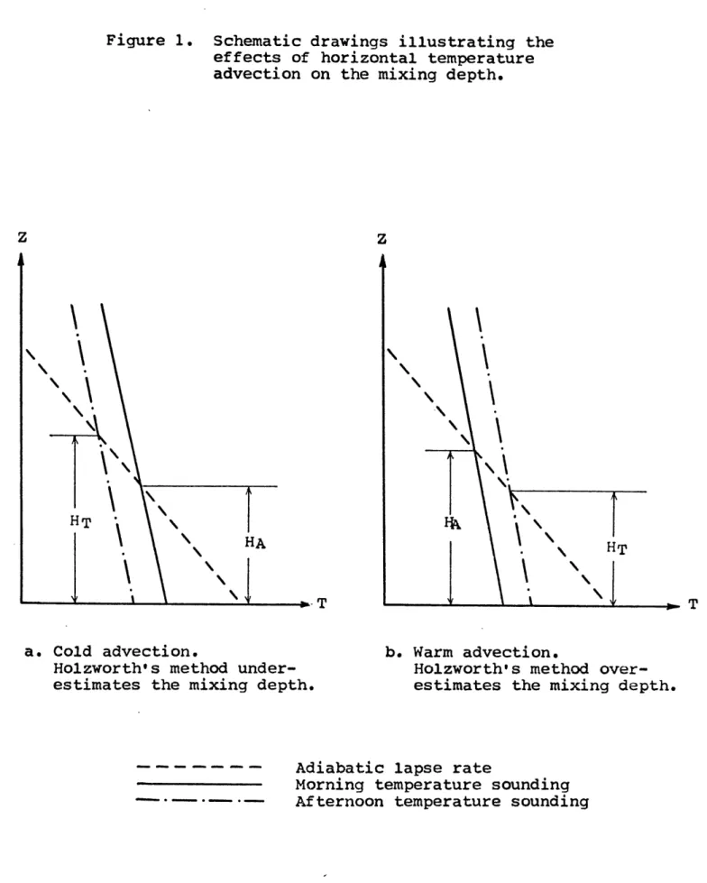
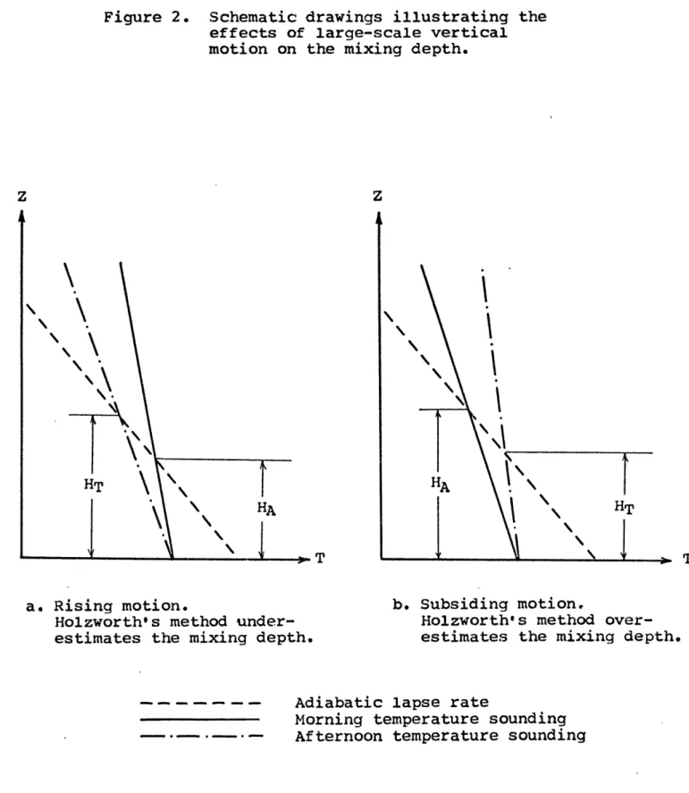
Figure


Documents relatifs
phytoplankton bloom, primary production, carbon deep export 44.. The subpolar winter regime is characterized by a deepening of the mixed layer 49.. by several hundreds of meters and
The river plume is then subject to frontal symmetric, baroclinic, barotropic and vertical shear instabilities in the coastal part, north of the estuary (its far field).. Con-
It is shown that by adding a suitable perturbation to the ideal flow, the induced chaotic advection exhibits two remarkable properties compared with a generic perturbation :
The test shows that in the presence of water and oil phases, compared with pure TCDDA surface, the composite surface of TCDDA + stearic-acid treated calcium
Dans un premier temps, nous avons identifié les mécanismes de dégradation des digues en remblai pouvant provenir d’une défaillance d’une infrastructure puis nous avons
When fertilization is concentrated in the first months after planting, nitrate leaching in deep soil layers might increase the heterogeneity of the stands since deep nitrates could
Compared to the decision metric previously proposed by Premus and Helfrick, 3 the main difference is that energy ratio is here computed in mode space, whereas they use projections
El manual Un mundo por descubrir es un libro para el aprendizaje y la enseñanza de español como lengua extranjera para alumnos del segundo curso de secundaria, y
