Publisher’s version / Version de l'éditeur:
Computers and Chemical Engineering, 29, April 5, pp. 1023-1039, 2005-04-01
READ THESE TERMS AND CONDITIONS CAREFULLY BEFORE USING THIS WEBSITE.
https://nrc-publications.canada.ca/eng/copyright
Vous avez des questions? Nous pouvons vous aider. Pour communiquer directement avec un auteur, consultez la première page de la revue dans laquelle son article a été publié afin de trouver ses coordonnées. Si vous n’arrivez pas à les repérer, communiquez avec nous à [email protected].
Questions? Contact the NRC Publications Archive team at
[email protected]. If you wish to email the authors directly, please see the first page of the publication for their contact information.
NRC Publications Archive
Archives des publications du CNRC
This publication could be one of several versions: author’s original, accepted manuscript or the publisher’s version. / La version de cette publication peut être l’une des suivantes : la version prépublication de l’auteur, la version acceptée du manuscrit ou la version de l’éditeur.
For the publisher’s version, please access the DOI link below./ Pour consulter la version de l’éditeur, utilisez le lien DOI ci-dessous.
https://doi.org/10.1016/j.compchemeng.2004.11.003
Access and use of this website and the material on it are subject to the Terms and Conditions set forth at Evaluating offshore technologies for produced water management using Greenpro-I - a risk-based life cycle analysis for green and clean process selection and design
Sadiq, R.; Khan, F. I.; Veitch, B.
https://publications-cnrc.canada.ca/fra/droits
L’accès à ce site Web et l’utilisation de son contenu sont assujettis aux conditions présentées dans le site LISEZ CES CONDITIONS ATTENTIVEMENT AVANT D’UTILISER CE SITE WEB.
NRC Publications Record / Notice d'Archives des publications de CNRC:
https://nrc-publications.canada.ca/eng/view/object/?id=2554c532-aaf8-40ea-9d1c-a3179a05b575 https://publications-cnrc.canada.ca/fra/voir/objet/?id=2554c532-aaf8-40ea-9d1c-a3179a05b575
Evaluating offshore technologies for produced water management using GreenPro-I – a risk-based life cycle analysis for green and clean process selection
and design
Sadiq, R.; Khan, F.I.; Veitch, B.
NRCC-47732
A version of this document is published in / Une version de ce document se trouve dans : Computers & Chemical Engineering, v. 29, no. 5, April 2005, pp. 1023-1039
DOI:10.1016/j.compchemeng.2004.11.003
Evaluating offshore technologies for produced water management using
GreenPro-I - a risk based life cycle analysis for green and clean process
selection and design
Rehan Sadiq1, Faisal I Khan2, and Brian Veitch
Faculty of Engineering and Applied Science, Memorial University of Newfoundland St. John’s, NL, Canada A1B 3X5
Abstract
Sustainable development and environmental protection require green products, processes, and waste management strategies. The selection and design of green and clean processes and products involve handling a huge set of data related to the environment, economics and technologies. Therefore, it is essential to employ a comprehensive technique to guide decision-making under uncertainty that can incorporate these factors.
The paper presents decision-making under uncertainty based on life cycle analysis and considering environmental, technological, and economical drivers in the analysis. The methodology, GreenPro-1, is applicable at any stage of a process design and can be used to evaluate the environmental burdens of a product or a process throughout its life cycle, and to identify and assess opportunities to make improvements. A weighting scheme is used to integrate various criteria and policies so that a most appropriate alternative can be selected.
The GreenPro-1 methodology is applied to a case study for offshore produced water management. In the first stage, fourteen best available technologies (BAT) for treatment of produced water are evaluated individually using cradle-to-gate life cycle analysis. In the second stage, seven treatment strategies are developed from BAT and are further investigated. A treatment strategy that combines a hydrocyclone and produced water re-injection proved to be the best system among selected
strategies. The combination of hydrocyclone and adsorption was found to be the next best treatment strategy. Two other noteworthy strategies were membrane and centrifuge combination, and down hole separation and injection.
Keywords: Green process design, process selection, decision-making, produced water, offshore, and life cycle analysis
1
Institute for Research in Construction, National Research Council, Ottawa, Ontario, Canada
2
1 Introduction
The prescriptive regulatory-based approach for process design is being replaced by goal-based environmental management activities. This has been initiated due to recognition that strict compliance with standards, which are periodically adjusted to accommodate new research findings and changing expectations of the community, is expensive and resource-intensive and does not necessarily result in a reduction of environmental risk. Consequently, there has been a growing interest in ways that can help shift an organization’s environmental management
program from a reactive to a proactive strategy that encourages the organization to move beyond compliance and is beneficial from business view point.
The shift from process or product-specific impacts to long-term system-wide subsidiary impacts has created interest in the use of life cycle analysis (LCA) – an evaluation technique that assesses the environmental impacts of a product or service from cradle to grave or cradle to gate. The LCA’s philosophy is to consider the true extent of the environmental burden, which can only be understood if the steps of a product’s production, use and disposal are accounted for in the analysis. The LCA framework can be used to identify and assess potential improvements at any stage of a product’s life. Growing acceptance of LCA by regulatory bodies and industries internationally has lead to the development of the ISO 14040 series of standards on environmental management (ISO 1998). The Society of Environmental Toxicology and Chemistry (SETAC) has proposed a framework for LCA based on an integrative approach to avoid substituting one set of environmental problems for another set of problems (UNEP 1996). Although both work independently, a general consensus on methodological frameworks has started to emerge.
In this paper, decision-making under uncertainty is performed using LCA, which considers environmental, technological and economical drivers in the analysis. GreenPro-1, a decision-making methodology previously developed (Khan et al. 2001; 2002), is applicable at any stage of a process design. In this paper, the GreenPro-1 is applied to a case study for offshore
produced water management. In the first stage, best available technologies (BAT) are evaluated for the treatment of produced water using GreenPro-1. In the second stage, seven treatment strategies are defined from the BAT options and are further investigated using GreenPro-1.
1.1 Approaches for process selection and design
Unlike traditional process selection and design in which engineers and designers focus on cheaper options, clean and green process selection and design highlight environmental
considerations (Figure 1). In general, process simulators provide local scale models to predict mass and energy flows around a chemical process. Costs linked with these performance models can predict the profitability of a process. The goals in terms of profitability are defined.
Researchers in academia and industry have been using simulators and modeling tools with defined environmental constraints to explore and improve profitability. Recently, Cabezas et al. (1997) proposed a Potential Environmental Impact (PEI) balance for the generalization of the Waste Reduction (WAR) algorithm introduced by Hilaly and Sikdar (1994). The PEI balance quantifies the environmental impact of the pollutants emitted in a process and determines the environmental friendliness of a given process. Cano-Ruiz and McRae (1998) have provided a comprehensive review of techniques used to incorporate environmental considerations into the process design. However, to handle conflicting objectives, a multi-objective approach is essential.
There are number of methods available for generating process alternatives. Hierarchical methods emphasize the use of heuristic techniques and approximate calculations (Douglas 1988). These methods initially emphasize the broad view and later focus at unit levels. Biegler et al. (1997) reviewed optimization methods for selecting process alternatives. Daichendt and Grossmann (1998) have described an integrated approach that combines hierarchical and optimization methods.
Chemical stressors emitted are classified based on specific environmental impacts, e.g., acid rain and smog formation. They are characterized for potential effects based on scoring methods e.g., WAR (Hilaly and Sikdar 1994) and SETAC (1993), which classify impact categories, and
characterize their effects using weighting factors. Young and Cabezas (1999) have later modified the original WAR algorithm to include the potential environmental impact computation for the energy use in the process. Kniel et al. (1996) used LCA for a case study of a nitric acid process and incorporated environmental and economical constraints. Hernandez et al. (1998) tried to achieve the optimal degree of pollution abatement through a modeling approach. Azapagic and
co-workers (1999a-d) recommended LCA based design for process (and product) selection to guide decision-making. Azapagic (1999) and Azapagic and Clift (1999b, c) used LCA for the evaluation of process performance. Fu et al. (2000) initially applied evaluation techniques in a design procedure using a simple spreadsheet analysis to highlight the impact categories, streams, and components of the greatest concern. Later on they analyzed economical and environmental impacts at an advanced stage of the process design or operation.
Attempts have been made to integrate LCA with public decision-making, but this is not yet accepted as a part of the regulatory process. The European Union’s eco-labeling schemes (Boustead 1992), the EC directive on Packaging and Packaging Waste (HMSO 1997), and the IPPC Directive (1996) are some examples in this direction.
Khan et al. (2001) proposed a methodology called GreenPro for the design problem formulation using LCA, and design problem solution using multi-objective optimization and multi-criteria decision-making (MCDM). Application of the methodology was demonstrated through a case study of a vinyl chloride monomer process (Khan et al. 2001). The GreenPro proved effective in design, but its application was restricted only to early stage design due to its extensive
computational load and large data requirements. Khan et al. (2002) overcame earlier limitations with a more flexible, and robust methodology, GreenPro-I, which is applicable for any design stage, even when the data are scarce and qualitative. The GreenPro-I is applied here for the evaluation of BAT treatment options for offshore produced water management. In the present pursuit, the GreenPro-I is modified using various ranking methods, which increase the robustness and confidence in decision-making.
2 GreenPro-I
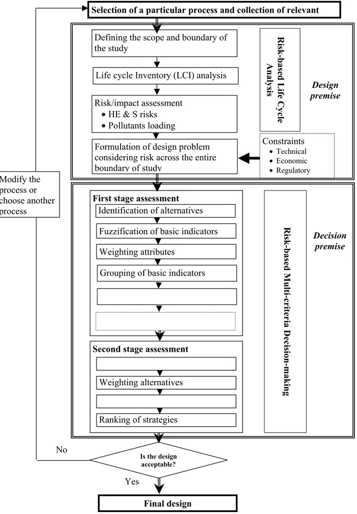
The GreenPro-I is comprised of two risk-based modules: 1) life cycle analysis and 2) multi-criteria decision-making. These two steps are further split into numerous sub-steps (see Figure 2). A step-by-step description of the methodology is presented here.
2.1 Risk-based life cycle analysis (RBLCA)
Risk-based life cycle analysis (RBLCA) is a process of weighting policy alternatives and
safety and economical risks quantitatively or qualitatively. RBLCA considers the complete material and energy supply chains within the system boundary. It includes material and energy flows into the system, outflows from the system, and consumption within the system. It classifies the environmental burden of all activities within the system boundary from material extraction (and/or excavation) to refining, transportation, construction and commissioning, production, and to decommissioning of the plant, and finally to the ultimate disposal. This module is comprised of four main steps, which are discussed below.
2.1.1 Scope and boundary
RBLCA defines the scope of the study and sets system boundaries. This requires backtracking from the conventional process system to the natural state of raw materials, which are available at no environmental penalty. Different technological routes for the production of the same set of raw materials should be included in the system boundary. The advantage of defining a global system boundary is that inputs (to the conventional process), together with their routes, can be accounted for with the output emissions forming an aggregated waste vector. Note that, although this definition is consistent with the conventional LCA, here it does not include the routes and stages of the product after leaving the process (cradle-to-gate).
2.1.2 Life cycle inventory (LCI)
The life cycle inventory (LCI) analysis is performed to collect data and quantify environmental loads (ELs) by making material and energy balances for each operation within the system. If the information is incomplete, the adopted data used in the analysis should be conservative and clearly reported. Data quality varies depending upon the source, therefore the selection of best available sources must be ensured.
The guiding principle for the LCI analysis is that all input and waste streams in a system (or subsystem) must be allocated to the respective non-waste output streams. When an output stream becomes an input stream to the next process step, it carries ELs into the next output streams. Therefore, the final products are assigned the sum of ELs of raw materials, energy, and wastes in this process chain. Figure 3 illustrates a general framework for life cycle inventory methodology.
2.1.3 Environmental impact and risk analysis
The environmental impact and risk analysis examines the potential or actual environmental and human health effects from the use of resources and waste releases. It is performed in three stages: classification, characterization, and valuation.
Classification is the process of assigning and aggregating results from the inventory into
homogeneous impact categories. This involves identifying stressors and organizing them with respect to impact on the ecosystem. For example, stressors CO, NOx, and CH4 have the potential for global warming. It may also include complex stressors and impact chains, because a single stressor has multiple impacts, and a primary impact can result in secondary (or greater) impacts. General categories are resource depletion, ozone depletion, acid rain potential, and health and safety risks related to human and ecological communities. These categories may change with the scope of the problem, however, the basic steps remain the same. In our case study, in addition to the above categories, the treatment efficiency parameters (dispersed oil, heavy metals, and others) are also considered.
Characterization assesses the impacts for each category in order to translate LCI data into impact
descriptors. Impact equivalency units are available for subsets of stressors. Where these are unavailable, new impact equivalency units must be established.
Valuation assigns relative importance values to different impacts to determine the total score for
each criterion. The valuation involves a structured description of the hierarchical relationships among the problem elements, beginning with an overall goal statement to developing a decision tree. Weights are estimated based on an expert panel who reach to consensus before using it for RBLCA. The expert panel may include economists, chemical and environmental engineers, and management representatives (see Khan et al. 2002 for details).
2.1.4 Design problem formulation
A traditional chemical process design requires knowledge of mass and energy balances,
thermodynamics, reaction engineering, and economics. Cabezas et al. (1997, 1999) incorporated environmental impacts (EI) into the process design through a mass balance. It is expressed mathematically by:
∂Isystem/∂t = Iincp + Iinep – Ioutcp - Ioutep- Iwecp- Iweep + Igenesystem (1) where Isystem is an amount of EI inside the system (chemical process is denoted by the superscript “cp” and energy generation process is denoted by “ep”); Iincp and Ioutcp are the input and output rates of EI to the chemical process; Iinep, and Ioutep are the input and output rates of EI to the energy generation process; Iwecp and Iweep are the outputs of EI associated with waste energy from the chemical and energy generation processes, respectively; and Igenesystem is the rate of generation of EI in the system. For steady state, this expression reduces to
0 = Iincp + Iinep – Ioutcp - Ioutep- Iwecp- Iweep + Igenesystem (2) It is necessary to relate the conceptual EI to measurable quantities. A generalized linear theory proposed by Mallick et al. (1996) and Cabezas et al. (1999) has been adopted in this study. It relates EI to measurable quantities such as stream flow rates, compositions and chemical specific environmental impacts (ϕk). The chemical specific environmental impact (ϕk) may be calculated using the WAR algorithm. The expression for chemical process is described as follows:
Iincp = Σ Ijin = Σ Mjin Σ Xjkϕk + … (3) Ioutcp = Σ Ijout = Σ Mjout Σ Xjkϕk + … (4) Iinep = Σ Ijin = Σ Mjin Σ Xjkϕk + … (5) Ioutep = Σ Ijout = Σ Mjout Σ Xjkϕk + … (6) where Ijcp is the rate of EI into or out of the chemical process; Ij is the EI flow rate with stream j, which may be an input or an output stream; Mj is the mass flow rate of stream j, which may be an input or an output; Xkj is the mass fraction of component k in stream j; and ϕk is the EI for chemical k. The same notation with superscript “ep” is used for energy production. In order to analyze the relationship between environmental impact and process cost, a mathematical framework has been used. The process is represented by a set of mathematical equations that describe the properties of the inlet stream, waste stream, and equipment specifications, cost functions and the degree of pollutant removal. This methodology uses the WAR algorithm to calculate basic chemical environmental impact and a modified WAR algorithm to calculate
energy related potential environmental impact. The details of WAR may be seen in Hilaly and Sikdar (1994) and the modified WAR in Young and Cabezas (1999).
The total EI of the system can be expressed by an environmental function like I = I (X). Any type of EI (e.g., global warming, and ozone depletion) can be incorporated into this function, usually as an environmental index. It allows all emissions from different compounds to be lumped together into a single number, which represents the impact. Thus, the environmental function is expressed as the sum of environmental impacts generated by both outputs and inputs from each species.
2.2 Risk-based multi-criteria decision-making (RBMCDM)
There are many approaches available for multi-criteria decision-making (Sadiq 2001).
GreenPro-I used fuzzy composite programming (FCP) which is briefly presented below (see
Sadiq et al. 2003 for details). A traditional MCDM problem can be expressed in a matrix form
mn 2 m 1 m n 2 22 21 n 1 12 11 X . . X X . . . . . X . . X X X . . X X m 2 1 A . A A n 1 1 X . . X X (7) where
Ai = 1, 2, ..., m are possible courses of action or alternatives;
Xi = 1, 2, ..., n are attributes, by which alternatives are measured; and
Xmn = Performance (rating) of alternative Ai with respect to attribute or criteria Xi. Often Xmn cannot be determined precisely due to unquantifiable, incomplete, or unobtainable information. Subjectivity may also arise due to ignorance of factual conditions. Unquantifiable information refers to subjectivity such as good, poor, high, and low. Examples of incomplete information are statements like about one million, and less than 10 km/h. Sometimes crisp data can be obtainable, but require a lot of resources, whereas approximation can be achieved with
less effort and time. Often linguistic descriptors are useful because of unavailability of
information or resources. Fuzzy set theory is an important tool to deal with these limitations and leads to fuzzy-based MCDM.
Fuzzy-based MCDM involves two main steps: aggregation and ranking. The aggregation determines the final utility value (performance score expressed by a fuzzy number) for each alternative by grouping the performance measures of the various individual attributes (criteria). In crisp MCDM, the final performance scores are real numbers, so the ranking is
self-explanatory. In fuzzy-based MCDM, the ranking involves ordering of the alternatives based on
defuzzification of a final utility value.
MCDM requires information about the relative importance of criteria involved in the analysis. In case of "n" criteria, a set of weights can be written as
(
)
1 1 2 1 ∑ = = = m j j n j T w , w ,...., w ,..., w , w W (8)By multiplying equation 7 with 8, the decision matrix becomes
D = Xij⊗ W = (9) × n 2 1 mn 2 m 1 m n 2 22 21 n 1 12 11 w . w w X . . X X . . . . . X . . X X X . . X X
Saaty (1988) proposed analytic hierarchy process (AHP) to estimate the relative weights of each attribute in a group based on pair-wise comparisons. Cheng and Lin (2002) defined linguistic variables for fuzzy importance factors (Table 1). The scale starts at very low, and goes on to low,
medium low, medium, medium high, high and very high. The higher the importance of an
attribute, the higher is the expected weight. The wj for each attribute in a group is given by:
∑ = = m j j j j Im Im w 1 (10)
where Imj is the importance factor, which can be selected from Table 1 for each attribute in a group. Chen and Hwang (1992) have provided eight scales to convert linguistic terms into fuzzy numbers. The same linguistic terms have different meanings in different scales. The principle of this system is to pick a scale that contains all verbal terms given by a decision-maker and use the fuzzy numbers in that scale to represent the meaning of verbal terms. We used Cheng and Lin’s (2002) linguistic variables (Table 1) to convert linguistic terms into fuzzy numbers.
2.3 Fuzzy composite programming (FCP)
It is important to select an appropriate RBMCDM strategy when the values of input variables, such as environmental risks, costs, and technical feasibility attributes are uncertain, or, vague. FCP is used to assist decision-makers in solving problems of multiple attributes and conflicting objectives with uncertainties. FCP is an extension of compromise programming (Bogardi and Bardossy 1983). Lee (1992) and Lee et al. (1991) used FCP for the management of dredged material disposal and for developing management strategies for nitrate control in drinking water, respectively. Stansbury et al. (1989) also conducted a risk-cost tradeoff study for dredged
materials disposal using FCP. Sadiq (2001) and Sadiq et al. (2003) used FCP for the
management of drilling waste disposal in the offshore to determine the best discharge scenario from risk, cost and technical feasibility viewpoints. Khan et al. (2002) used FCP for selecting the best source of energy for urea production.
2.3.1 Aggregation
FCP is a step-by-step procedure of grouping basic indicators to form generalized indicators. The cost, technical feasibility, environmental damages, and treatment efficiency parameters are defined as basic indicators. The first step in FCP is the normalization of the basic indicators to convert non-commensurate indicators into unitless entities. This is necessary because all basic indicators have different units and are difficult to compare in their respective units. The
efficiency of removal of dispersed oil, Benzene, Toluene, Ethyl benzene, and Xylene (BTEX), Poly-cyclic aromatic hydrocarbons (PAH), Naphthalene, Phenantherene, and Dibenzothiophene (NPD), heavy metal, and naturally occurring radioactive material (NORM) present in produced water can be grouped into a index for treatment efficiency. The environmental parameters - global warming, air pollution, critical water mass, and solid waste mass - can be combined into a
generalized group environmental index. The index for technical feasibility is obtained by grouping basic indicators like ease of operation, efficiency, status of technology and control measures. The grouping of different attributes is performed in steps to get the final system index. This trade-off analysis for different alternatives can be made at different hierarchy levels. The value of the (Level 3) system index represents the contributions of the grouped indexes at Level 2 (see Figure 4).
By defining Zi (x) as a fuzzy number of the ith basic indicator with a triangular membership function of µ[Zi (x)], various management alternatives under uncertainty can be evaluated. The confidence level for an uncertain value can be determined using observed or measured
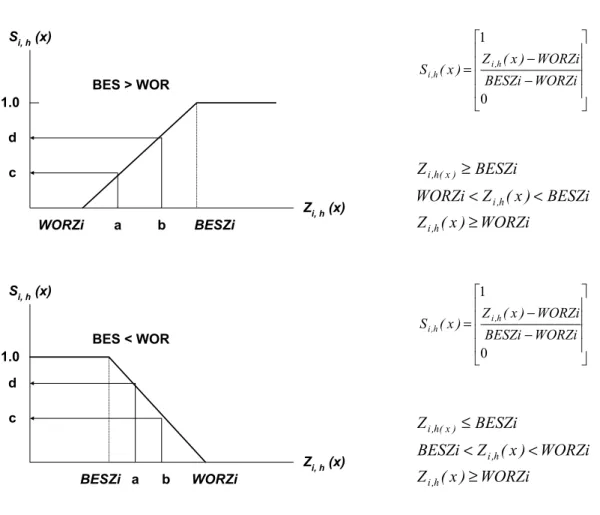
variability. Since units of basic indicators are different, the actual value of each basic indicator should be transformed into an index, Si,h(x), using the best (BES) or the worst (WOR) value of the indicator as shown in Figure 5 (Lee et al. 1991). Using the normalized index values of basic indicators, the Level 2 index values, Lj,h (x), of composite indicators can be defined by
[
∑ = = nj i j i,h,j h , j (x) w S (x) L 1]
(11)The variables are defined in the nomenclature. The index value Lk,h (x), of a third level composite indicator can be calculated by the index values of the second level composite indicators -
environment, cost, treatment efficiency and technical feasibility. The wj values are estimated using equation 10.
2.3.2 Ranking
The final performance rating determines how well an alternative satisfies the decision-maker's utility. The alternative with the highest rating will be most desirable. If the final ratings are real numbers, then it is straightforward to decide the best alternative.
Performance ratings Xij can be crisp, fuzzy, and/or linguistic. When fuzzy data are incorporated into MCDM, the final ratings will be fuzzy numbers, not crisp, which are not straightforward to compare. In MCDM applications when the final ratings are fuzzy, different ranking methods can be used. Chen and Hwang (1992) have classified ranking methods into four major groups:
preference relation, fuzzy mean and spread, fuzzy scoring, and linguistic expression. Fuzzy scoring techniques are the most popular. In the present study, we used three methods for ranking: Chen’s ranking method, simple averaging method, and weighted averaging method. For details refer to Chen (1985), Cheng and Lin (2002), and Khan et al. (2002).
In the case of group decision-making, there are different techniques available for the aggregation of preferences (Smolikova and Wachowiak 2002). In this study, an additive ranking rule is employed to arrive at a robust ranking order. The additive ranking rule determines the average ranking order of an alternative (Ai), which is the arithmetic mean of the rankings made by all ranking methods. m i N K Ai,K N Ai N R rank R ∈ = ∑ = 1 (12)
The parameters of the above equation are defined in the nomenclature.
2.3.3 Second stage assessment for comparing strategies
The second stage analysis is performed if r numbers of alternatives are combined and described as a strategy. The results of the first stage analysis are grouped at the highest hierarchy level using equal weights. The strategy (Sr) can be established as
( )
A W( )
A W( )
r Ar W1 ⋅ 1 + 2 ⋅ 2 +⋅ ⋅⋅+ ⋅ (13) r S = where W(1) and W(2) = 0.50, if r = 2W(1), W(2) and W(3) = 0.33, if r = 3 and so on.
3 Produced Water Management
Produced water is a byproduct of the production of oil and gas. Water is naturally present in the reservoirs and, despite all efforts to produce the hydrocarbons selectively, some water is
produced, admixed as a liquid with the oil or as vapor in the hydrocarbon. Produced water contains dispersed oil and dissolved organic compounds, including light aromatic hydrocarbons such as BTEX, PAH, heavy aromatic NPD, organic acids, phenols, inorganic compounds, as well as traces of NORM. The chemical composition varies over a wide range and depends mainly on the attributed to the reservoir's geology. The composition of produced water may also change slightly through the production life of a reservoir. After a couple of years, wells start producing increased quantities of water of almost stable composition. However, if water is injected for pressure maintenance, or for any other reason, the composition of produced water changes, due to dilution of the reservoir water. This would displace the water composition from equilibrium and create the potential for additional dissolution of aromatics from the oil phase (O&G 2002).
Produced water from oil production fields differs from gas production fields. Water from gas production fields generally has a higher content of low molecular weight aromatic hydrocarbons than water from oil production platforms. However, the total amount of water produced from gas fields is considerably smaller than oil production fields.
3.1 Fate of offshore produced water
Most aromatic compounds in produced water are volatile. They readily evaporate from the sea surface or from produced water plumes that reach the surface due to density gradients. The depressive mixing results in a 50-150 × 103 -fold reduction of the benzene concentration in seawater 20m away from the point of discharge (Rabalais et al. 1991; Tetrens and Tait 1996; Furuholt and Kinn 1996; Riksheim and Johnsen 1994; O&G 2002). The NPD compounds are less volatile, but still are reduced by evaporation. This is particularly important for high-temperature produced water discharges, or for produced water with a gas/air injection before discharge. The less water-soluble fraction of aromatic compounds, the PAH compounds, is expected to be associated with particulate and oil droplets and is likely to follow the plume, or be retained at certain depths of the water column depending upon the buoyancy of the supporting particulate matter.
Past studies in the North Sea revealed that PAH concentration levels exceeding the toxicity threshold levels can be found within a distance of 500m from the discharge point and may vary
spatially and temporally depending on the hydrodynamics (O&G 2002). The regulatory threshold limit is only dependent on the discharge concentration. In general, a dilution factor of 1000 or less is assumed sufficient to reach predicted no-effect concentration for PAH (OOC 1997). There are many technologies available for the treatment of dispersed and dissolved oil, and other wastes in produced water. Applicability of these technologies to produced water treatment must consider time, space, load, and vulnerability limitations. This study aims to evaluate different treatment options and a brief description of the BAT options is presented in the following section (for details see O&G 2002).
3.2 Treatment technologies
Three methods are used to reduce and control potential environmental impacts of produced water:
1. Avoid water production from the well. The production of formation and connate waters may be controlled, but equilibrium water due to condensation can not be avoided;
2. Re-injection. After surface separation of the water from the hydrocarbons, the water may be reinjected back into the formation. This technique is only possible when a well is available for disposal; and
3. Removal of hydrocarbons from the water. This can be done at several steps between the well bottom and discharge point.
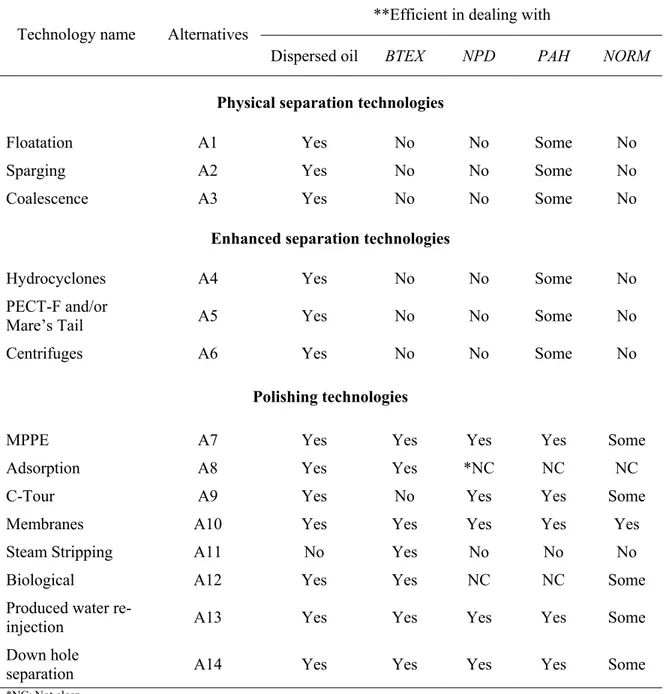
Methods 2 and 3 are discussed in the present paper. A range of technologies exists for the treatment of offshore produced water, and many of them are referred to as BAT. The key technologies evaluated in this paper are summarized in Table 2.
3.2.1 Physical separation
The majority of the technologies in this group remove dispersed oil and PAHs to a certain extent. However, the performance achieved by each system will depend on the process variables at each installation. These variables include reservoir type, temperature, pressure, oil type and viscosity,
emulsion stability, oil droplet size, water salinity, flow rate etc. The technologies in this group have limitations on efficiency, weight, size and processing time.
3.2.2 Enhanced separation
Further removal of dispersed oil can be obtained by enhanced separation after modifying the oil droplet characteristics in the upstream feed to the primary treatment system. This includes the use of mechanical coalescing systems (Pect-F, Mare's tail) and other commercially available technologies such as centrifuges and hydrocyclones.
Limitations to this technology for offshore operations are weight and space. The application of hydrocyclones (most widely used in the oil industry) enables large water volumes to be
processed, often without needing additional power input or chemicals. The residence time for hydrocyclones is very short (often in seconds), but reduces size, weight and cost of the treatment facilities significantly.
3.2.3 Polishing
Polishing technologies are suitable for the removal of dissolved aromatic hydrocarbons. The advantages and disadvantages of several polishing technologies are briefly discussed here. The details of the technology presented below are adopted from O&G (2002).
Hydrocarbon contaminated water is passed through a column packed with Macro Porous Polymer Extraction (MPPE) particles. An extraction liquid immobilized within the polymer matrix removes the hydrocarbons from the water. The purified water passes out of the column directly for reuse or discharge. Adsorption is a process in which a soluble contaminant (the adsorbate) is removed from water by contact with a solid surface (the adsorbent). The binding to the surface is usually weak and reversible. C-Tour process system is an enhancement to
hydrocyclone technology, which extracts hydrocarbons from water using gas condensate. The injected gas condensate acts as an extraction-solvent. The solvent extracts the dissolved hydrocarbons from the water phase and is later removed in the hydrocyclone. Membrane removes dissolved hydrocarbons at the molecular level. All hydrocarbons larger than the membrane material will be rejected (including dispersed oil). Steam stripping and distillation is
based on vapor-liquid equilibrium. In a typical stripper column, a vapor stream enters at the bottom while the liquid enters from the top. The vapor stream, which could be steam, air or any other gas, picks up the most volatile components in the liquid stream. Biodegradation employs microbes to break down and remove oil and aromatics from produced water. The processes require a medium to long residence time for the organisms to grow and stabilize for effective operation. After separation of the water and oil, produced water can be injected into a disposal well or preferably the same reservoir from where it originated. This process alone does not enable an operator to meet performance standards in the portion of produced water being discharged.
3.5 Offshore treatment strategies
Different treatment technology alternatives are efficient in the removal of different pollutants and complement each other by enhancing the treatment efficiency if used in series or parallel.
Various treatment alternatives can be grouped to develop a complete treatment strategy. Seven treatment strategies are identified in Table 3, which are evaluated in the second stage assessment of the proposed methodology.
4 Application of GreenPro-I 4.1 First stage assessment
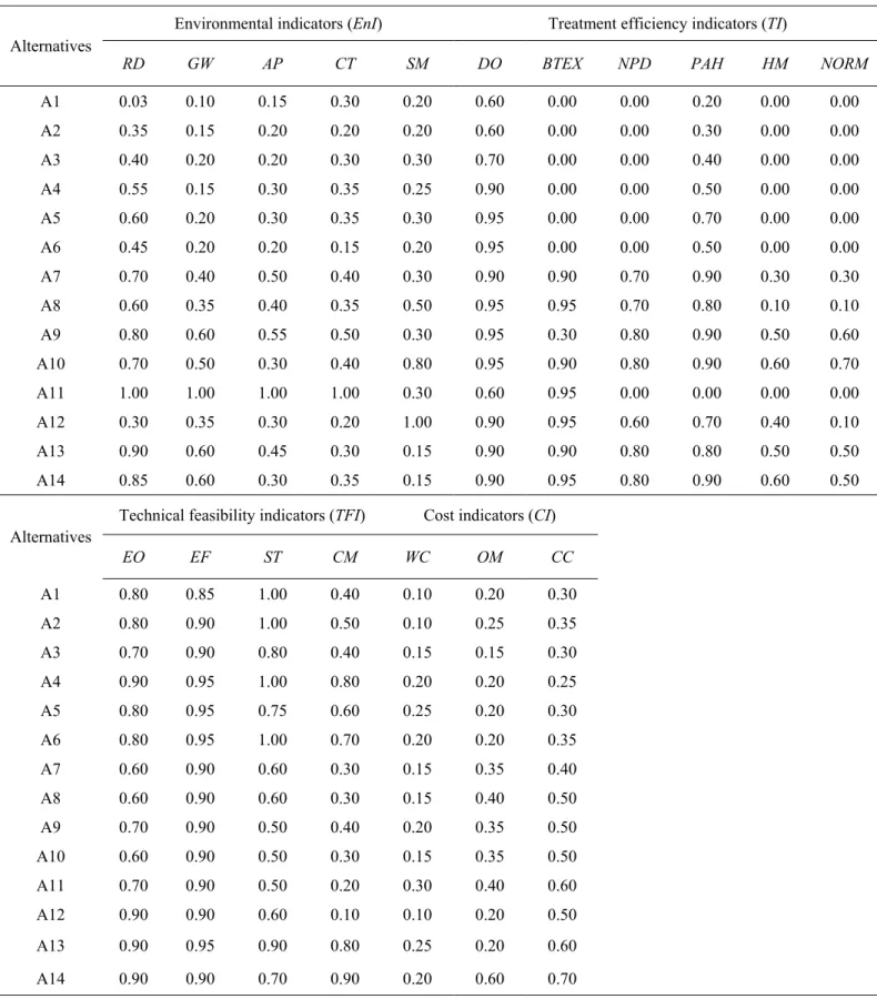
Fourteen treatment technology options were evaluated individually in the first stage assessment (Table 2). The GreenPro-I was applied to each treatment option to estimate the utility function (Ut) as described before. The available data for various basic indicators are either quantitative or qualitative in nature (Figure 4).
As a first step of this assessment, environmental impact for chemicals and energy use was calculated for all the fourteen treatment options using the WAR algorithm. In the environment category, five main impacts (resource depletion, global warming, air pollution, critical water mass, and critical solid mass) were estimated (Table 4a). The same approach is used to compute the treatment category performance impacts for dissolved oil, BTEX, NPD, PAH, Heavy metal, and NORM. Four qualitative parameters related to technical feasibility and three parameters
related to cost factors were also determined.
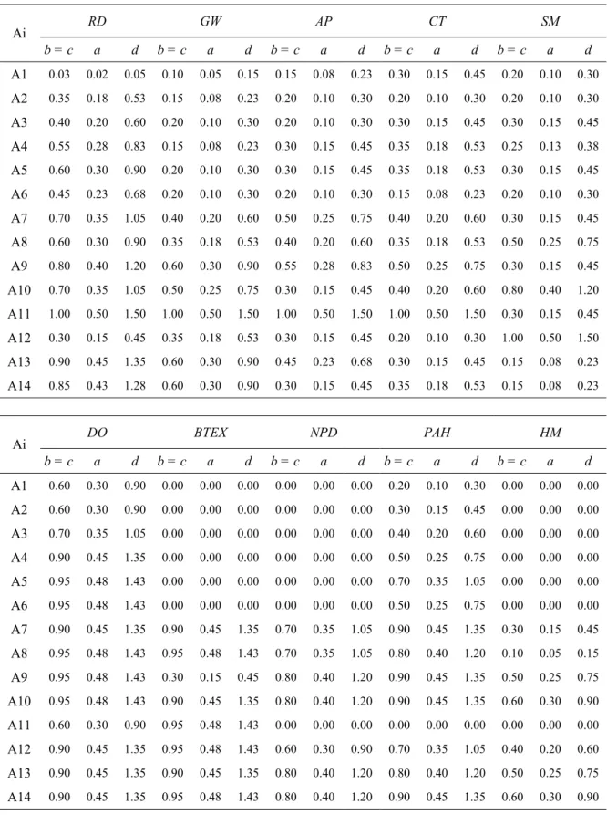
As the original input data were non-commensurate the normalization was carried to bring all parameters in the same scale. The normalization was dome using either cost (WOR > BES) or benefit (BES > WOR) criteria depending on its type. The WOR > BES represents those
indicators for which worst values are more than their best values, e.g., risk and cost. The BES > WOR represents those indicators for which best values are more than their worst values, e.g., technical feasibility (see Sadiq 2001 for details). The normalization process used here is illustrated in Figure 5.
The maximum likely estimates reported in Table 4a (developed with the help of O&G, 2002 data and WAR and its derivative algorithm) were fuzzified. The uncertainty in the normalized scale (b = c; maximum likely estimate) was expressed by a factor of ± 50% representing the largest likely interval between a and d (base of a triangular fuzzy number). The normalized triangular fuzzy data are reported in Table 4b.
To develop a weight or priority matrix, the importance scales (Imj) were assigned to various basic indicators (at level-I) and sub-attributes (at level-II) as given in Table 1. These importance factors were converted into normalized weights (wj) using equation 10. The weighting scheme for the first stage assessment is given in Table 5. The fuzzy composite structure described in Figure 4 was used to group indicators at two hierarchical levels.
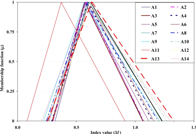
Figure 6 describes the system index of various treatment technologies after the first stage assessment. The bigger base of the TFN represents higher uncertainty in the system index.
Different ranking methods (described in the previous section) were used for defuzzification of the system index. The alternatives A10, A12 and A13 were found to be at the top of the list (Table 6). The comparison of treatment technologies from different categories (physical and enhanced separation, and polishing techniques) are compared. To make a comparison of commercially available technologies which are generally used in series, we performed a second stage assessment.
4.2 Second stage assessment
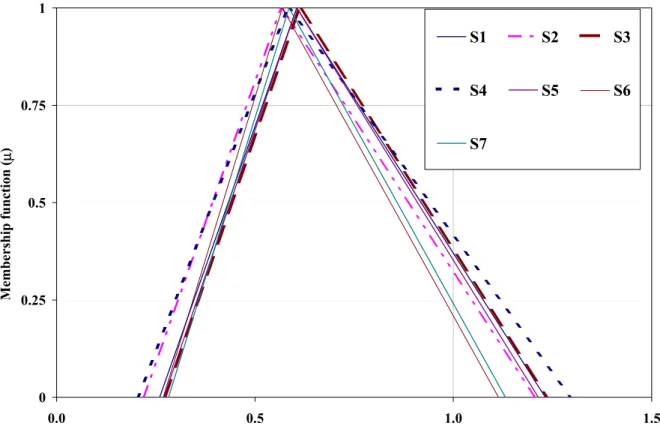
technologies) were established based on the result of the first stage assessment. These strategies are listed in Table 3. The proposed strategies were evaluated using the same procedure as followed in the first stage assessment. The indices obtained from the evaluation of these strategies are shown in Figure 7. Three ranking methods were employed to establish the final ranking order for these seven proposed strategies (Table 7).
The treatment strategy S3 (hydrocyclone and produced water re-injection) was found to be the best treatment system available and is rated best. The two technologies involved in this strategy are well tested and are currently in practice. Furthermore, the operating cost and environmental impacts of these technologies are the lowest. The treatment strategy S1 (hydrocyclone and adsorption) was also found to be among best treatment options available. This is also
commercially available technology. The strategy, S5 (membrane and centrifuge) was rated 3rd among the seven strategies, but extensive data were not available. Strategy S4 (down hole separation and injection) - a clean option of produced water management - was also very close. However, due to some unresolved technical and regulatory issues this technology has not been well practiced.
The ranking order obtained using this methodology is not necessarily fixed. Where more detailed data and information becomes available, the methodology developed here can help in
re-evaluating the alternatives (or strategies) in the light of emerging information. The intention here is to show the methodology, which has the flexibility to incorporate qualitative and quantitative data, and yet is comprehensive enough to guide in decision-making for product and process selection and design.
5 Summary and Conclusions
In green and clean process selection and design, different alternatives are evaluated. These alternatives may be basic conceptual designs of the process or techniques or technologies of waste management. Each alternative would result in a different set of (environmental,
economical, and technological) data. These data must be evaluated to select or design a process, product or waste management strategy. Therefore, it is required to adopt or develop a simple but comprehensive technique for design decision-making that can incorporate all these factors (data). In this regard, a few methodologies have been proposed in the literature. GreenPro and
GreenPro-1 are flexible enough to apply for any design stage. In this paper, GreenPro-I is
revisited and applied to a case study of offshore produced water management for the evaluation of BAT options.
In the first stage assessment, fourteen BAT options were evaluated considering the cradle to gate life cycle analysis. In the second stage assessment, seven treatment strategies were developed by utilizing the results of the first stage assessment. The treatment strategy combining a
hydrocyclone and produced water re-injection was found to be the best treatment system available. The two technologies involved in this strategy are well tested and are in current practice. The ranking order obtained using this methodology may change by incorporating more precise data. The intention of this paper is to demonstrate the new methodology, which is flexible enough to incorporate qualitative and quantitative data in guiding decision-making for product and process selection and design.
Readers are encouraged to contact for their comments or views to: Dr. Rehan Sadiq ([email protected]) and Dr. Faisal Khan ([email protected]).
Nomenclature
Ai An alternative
Ij Environmental impact flow rate with stream j
Imj Importance factor of attribute j
Isystem Environmental Impact within the system
Iin Input rates of environmental impact to the system (chemical process or energy
generation)
Iout Output rates of environmental impact form the system (chemical process or energy
generation)
Iwe Output rate of environmental impact associated with waste energy from the system
(chemical and energy generation processes)
Igene Rate of generation of environmental impact in the system
K Ranking methods (1 – N)
Lk,h (x) Third level composite indicator
Mj Mass flow rate of stream j
N Total number of ranking methods
nj Number of elements in second-level group j
rank( value)i ∈ m Operator convert the alternative Ai into ranking order among m alternatives N
Ai
R = Average ranking order of an alternative Ai
Si,h,j (x) Basic value for ith basic indicator in the second level group j of basic indicators
with membership of h;
wj, Wj Weight reflecting importance basic indicator (or attribute) in group j
Xi Attributes by which alternatives are measured
Xkj Mass fraction of component k in stream j
Xmn Performance (rating) of alternative Aiwith respect to attribute or criteria Xi
Zi (x) Fuzzy number of the ith basic indicator with a triangular membership function
µ[Zi (x)], Fuzzy triangular membership function
ϕk Environmental impact for chemical k
Superscripts
system system
cp chemical process
Acronyms AHP Analytical hierarchy process
AP Air pollution
BAT Best available technology
BTEX Benzene, Toluene, Ethyl benzene, and Xylene
CC Capital cost
CM Control measures
CT Critical water mass
DO Dissolved oil
EF Efficiency
EI Environmental impact
EL Environmental Lload
EnI Environmental indicator
EO Ease of operation
FCP Fuzzy composite programming
GW Global warming
HE & S Human ecological and safety
HM Heavy metals
ISO International standardization organization LCA Life cycle analysis
LCI Life cycle inventory
MCDM Multi-criteria decision-making
MPPE Macro porous polymer extraction NORM Naturally occurring radioactive material
NPD Napthelene, Phenantherene, and Dibenzothiophene
OD Ozone depletion
OM Operation & maintenance
PAH Poly-cyclic aromatic hydrocarbons PEI Potential environmental impact RBLCA Risk-based life cycle analysis
RBMCDM Risk-based mMulti-criteria decision-making
RD Resource depletion
SETAC Society of environmental toxicology and chemistry SI System score or index
SM Solid waste mass
ST Status of technology
TFI Technical feasibility index TFN Triangular fuzzy number TI Treatment efficiency index
WAR Waste reduction
6 References
Azapagic, A., and Clift, R., (1999a). Linear Programming as a Tool in Life Cycle Assessment,
International J. of LCA, 4(6), 305-316.
Azapagic, A., and Clift R., (1999b). Allocation of Environmental Burdens in Multiple-Function Systems, J. Cleaner Production, 9(2), 101-119.
Azapagic, A., and Clift, R., (1999c). The Application of Life Cycle Assessment to Process Optimization, Computers and Chemical Engineering, 23, 1509-1526.
Azapagic,A., and Clift, R., (1999d). Life Cycle Assessment as Tool for Improving Process Performance: A Case Study on Boron Products, Int. J. LCA, 4(3), 133-142.
Azapazic, A., (1999). Life Cycle Assessment and its Application to Process Selection, Design and Optimization, Chemical Engineering Journal, 73, 1-21.
Biegler, L.T., Grossmann, I.E., Siirola, J.J., Westerberg, A.W., (1997). Systematic Methods of Process Design, Prentice Hall, NY, pages 700.
Bogardi, I. and Bardossy, A., (1983). Application of MCDM to Ggeological Eexploration, In:
Essays and Surveys on Multiple Criterion Decision-Making, Henson, P. (Ed.),
Springer-Verlag, NY.
Boustead, I., (1992). Eco-balance Methodology for Commodity Thermoplastics, PWMI, Brussels.
Cabezas, H., Bare, C.J., and Mallick, S.K., (1997). Pollution Prevention with Chemical Process Simulators: The Generalized Waste Reduction (WAR) Algorithm, Computers in Chemical
Engineering, 21, s305-s310.
Cabezas, H., Bare, C.J., and Mallick, S.K., (1999). Pollution Prevention with Chemical Process Simulators: The Generalized Waste (WAR) Algorithm-full Version, Computers in Chemical
Engineering, 23, 625.
Cano-Ruiz, A. and McRae, G.J., (1998). Environmentally Conscious Process Design, Annual
Review of Energy and the Environment, vol. 23, November 1998.
Chen, S. H., (1985), Ranking Fuzzy Numbers with Maximizing Set and Minimizing Set, Fuzzy
Set Systems, 17(2), 113-129.
Chen, S.J., and Hwang, C.L., (1992). Fuzzy Multiple Attribute Decision-Making, Springer-Verlag, NY.
Cheng, C-H, and Lin, Y., (2002). Evaluating the Best Main Battle Tank Using Fuzzy Decision Theory with Linguistic Criteria Evaluation, European J. Operational Research, 142, 174-186.
Daichendt, M.M. and Grossmann, I.E., (1998). Integration of Hierarchical Decomposition and Mathematical Programming for the Synthesis of Process Flow sSheets, Computers and
Chemical Engineering, 22, 147-175.
Douglas, J.M., (1988). Conceptual Design of Chemical Processes, McGraw-Hill, NY, 601 pp. Fu, Y., Diwekar, U.M., Young, D., and Cabezas, H., (2000). Process design for the environment:
a multiobjective framework under uncertainty, Clean Products and processes, 2, 92-107 Furuholt, E., and Kinn, S.J., (1996). Regional Environmental Impact Assessment, SPE paper
SPE -46470, HSE meeting in 1998, Caracas, Venezuela.
Hernandez, O. R., Pistikopoulos, and Livingston, A.G., (1998). Waste Treatment and Optimal Degree of Pollution Abatement, Environmental Progress, 17(4), 270-276.
Hilaly, A. K. and Sikdar, S.K., (1994). Pollution Balance: A New Methodology For Minimizing Waste Production In Manufacturing Processes, J. Air Waste Manage. Assoc., 44, 1303-1315. HMSO, (1997). Producer Responsibility Obligations (packaging waste) Regulations, London. IPPC Directive, (1996). EU Council Directive 96/61/EC of 24 September 1996 Cconcerning
Iintegrated Ppollution Pprevention and Ccontrol, Official Journal L 257, 10/10/1996 P. 0026
– 0040.
ISO 14001, (1998). Environmental Mmanagement Ssystems – Llife Ccycle Aassessment–
Pprinciples and Fframework, International Standardization Organization; Geneva. ISO,
(1998).
Khan, F.I., Natrajan, B.R., Revathi, P., (2001). GreenPro: A New Methodology for Cleaner and Greener Process Design, J. Loss Prevention in the Process Industries, 14, 307-328.
Khan, F.I., Sadiq, R., and Husain, T., (2002). GreenPro-I: A Methodology for Risk-Based Process Plant Design Considering Life Cycle Assessment, J. Environmental Modeling &
Software, 17, 669-692.
Kniel, G.E., Delmarco, K., and Petrie, J.G., (1996). Life Cycle Assessment Applied to Process Design: Environmental and Economic Analysis and Optimization of a Nitric Acid Plant,
Environmental Progress, 15(4), 221-228.
Lee, Y.W., (1992). Risk Assessment and Risk Management for Nitrate Contaminated
Groundwater Supplies, Ph.D. Dissertation, Department of Civil Engineering, University of
Nebraska, Lincoln, Nebraska.
Lee, Y.W., Bogardi, I. and Stansbury, J., (1991). Fuzzy Decision-Making in Dredged Material Management, Journal of Environmental Engineering, ASCE, 117(5), 614-630.
Mallick, S.K., Cabezas, H., Bare, J.C., and Skidar, S.K., (1996). A Pollution Reduction Methodology for Chemical Process Simulators, Industrial Engineering and Chemical
Research, 35, 4128.
O& G, (2002). Aromatics in Produced Water: Occurrence, Fate and Effects, and Treatments,
Report number I.20/324, International Association of Oil and Gas Producers, London, UK.
OOC, (1997). Gulf of Mexico Produced Water Bioaccumulation Study. Offshore Operators Committee, PO Box 50751, New Orleans. Offshore Operator’s Committee.
Rabalais, N.N., Turner, R.E., Wiseman Jr., W.J. , and Boesch, D.F., (1991). A Brief Summary of
Hypoxia on the Northern Gulf of Mexico Continental Shelf: 1985-1988. In: Tyson, R.V. and
T. H. Pearson (Eds.), Modern and ancient continental shelf anoxia. Geological Society special publication no. 58. London: The Geological Society. pp. 35-46.
Riksheim, H., and Johnsen, S., (1994). Determination of Produced Water Constituents in the Vicinity of Production Fields In The North Sea, SPE- paper 27150, SPE conference, Jakarta. Saaty, T.L., (1988). Multi-Criteria Decision-Making: The Analytic Hierarchy Process,
University of Pittsburgh, Pittsburgh, PA.
Sadiq, R., (2001). Drilling Waste Discharges in the Marine Environment: A Risk Based Decision
Methodology, Ph.D. Thesis, St. John's, Memorial University of Newfoundland, Canada.
Sadiq, R., Husain, T., Veitch, B., and Bose N., (2003). Risk Management of Drilling Waste Disposal in the Marine Environment - A Holistic Approach, Oceanic Engineering
International, 7(1), 1-22.
SETAC, (1993). Guidelines for Life-Cycle Assessment: A Code of Practice, Society of Environmental Toxicology and Chemistry, Pensacola, FL, pages 15.SETAC, (1993). Smolikova, R., and Wachowiak, M.P., (2002). Aggregation Operators for Selection Problems,
Fuzzy Sets and Systems, 131, 23-24.
Stansbury, J., Bogardi, Kelly W. E., (1989). Risk-Cost, Analysis for Management of Dredge Material, In: Risk-Based Decision-Making in Water Resources, Proceedings of the 4th
Conference Sponsored by the Engineering Foundation, American Society of Civil Engineers.
Terens Terrends, G.W. and Tait, R.D., (1996). Monitoring Ocean Concentration of Aromatic Hydrocarbons from Produced Formation Water Discharges to Bass Strait Australia, SPE-36033, 3rd SPE Health Safety and Environmental Conference, New Orleans.
UNEP, (1996). Life Cycle Assessment: What It Is and How to Do It?, United Nations Environment Program, Industry and Environment United Nations Publication, Geneva. Young, D.M., and Cabezas, H., (1999). Designing Sustainable Processes with Simulation: the
Design Objectives Environment impacts Regulatory compliance Safety Economics
Life cycle consideration
Process Simulation Chemical synthesis Process Synthesis Process integration Cost Reduction Final Process Improved environment and energy performance
Defining the scope and boundary of the study
Formulation of design problem considering risk across the entire boundary of study
Fuzzy ranking for various Sensitivity analysis (optional)
Identification of strategies
Grouping of alternatives
Final design
Figure 2. Basic framework for modified GreenPro-I (Khan et al. 2002) Constraints • Technical • Economic • Regulatory Ranking of strategies Weighting alternatives Second stage assessment
Weighting attributes Modify the process or choose another process No
Selection of a particular process and collection of relevant
Is the design acceptable?
Design premise
Risk-based Life Cycle
Analysis
Risk/impact assessment
• HE & S risks
• Pollutants loading
Life cycle Inventory (LCI) analysis
Grouping of basic indicators
Decision premise
Risk-based Multi-criteria Decis
ion-making
Fuzzification of basic indicators
Yes
First stage assessment Identification of alternatives
Process Description
Collect all relevant data
Identify all possible Hazards
Identify release scenarios
Compute environmental load
Ignore this scenario and select other scenario No
Is the estimated load substantial?
Yes
Perform detailed risk and impact assessment
Add these risk and impact factors to compute global impact and risk factors Select another scenario
No Are all scenarios studied?
Select another hazard Yes
No Are all hazards assessed? Yes
Report total Global Risk and Impact
Level 1 Level 2 Level 3
Grouping various BAT options to de
velop management strategies
Second stage assessment First stage assessment
Resource Depletion
Environment
Critical Solid Mass Critical Water Mass Air Pollution Global Warming NORM Heavy Metal PAH NPD BTEX Dissolved Oil Treatment Cost Capital Cost
Opt. & Maintenance Working Capital Technical Feasibility Control Measures Technology Status Efficiency Ease of Operation System
WORZi BESZi Si, h (x) a b c d 1.0 Zi, h (x) BES > WOR − − = 0 1 WORZi BESZi WORZi ) x ( Z ) x ( Si,h i,h WORZi ) x ( Z BESZi ) x ( Z WORZi BESZi Z h , i h , i ) x ( h , i ≥ < < ≥ WORZi BESZi Si, h (x) a b c d 1.0 Zi, h (x) BES < WOR − − = 0 1 WORZi BESZi WORZi ) x ( Z ) x ( Si,h i,h WORZi ) x ( Z WORZi ) x ( Z BESZi BESZi Z h , i h , i ) x ( h , i ≥ < < ≤
0 0.25 0.5 0.75 1 0.0 0.5 1.0 1
Index value (SI )
Membership function ( µ ) A1 A2 A3 A4 A5 A6 A7 A8 A9 A10 A11 A12 A13 A14 .5
0 0.25 0.5 0.75 1 0.0 0.5 1.0 1.5
Index value (second stage assessment)
Membership f unct ion ( µ ) S1 S2 S3 S4 S5 S6 S7
Table 1. Linguistic measures of importance
Intensity of importance, Imj *Definition (TFN)
Very low (VL) (0, 0.05, 0.1) Low (L) (0.1, 0.18, 0.25) Medium low (ML) (0.25, 0.33, 0.4) Medium (M) (0.4, 0.5, 0.6) Medium high (MH) (0.6, 0.68, 0.75) High (H) (0.75, 0.83, 0.9) Very high (VH) (0.9, 0.95, 1)
Table 2. Details of the technology investigated in present study (modified after O&G 2002)
**Efficient in dealing with
Technology name Alternatives
Dispersed oil BTEX NPD PAH NORM
Physical separation technologies
Floatation A1 Yes No No Some No
Sparging A2 Yes No No Some No
Coalescence A3 Yes No No Some No
Enhanced separation technologies
Hydrocyclones A4 Yes No No Some No
PECT-F and/or
Mare’s Tail A5 Yes No No Some No
Centrifuges A6 Yes No No Some No
Polishing technologies
MPPE A7 Yes Yes Yes Yes Some
Adsorption A8 Yes Yes *NC NC NC
C-Tour A9 Yes No Yes Yes Some
Membranes A10 Yes Yes Yes Yes Yes
Steam Stripping A11 No Yes No No No
Biological A12 Yes Yes NC NC Some
Produced water
re-injection A13 Yes Yes Yes Yes Some
Down hole
separation A14 Yes Yes Yes Yes Some
*NC: Not clear
Table 3. System of treatment strategies- second stage assessment
Strategy System of technologies Comments
S1 Hydrocyclone + Absorption Commercially available and known as MPPE based
technology (A7)
S2 Hydrocylcone + Solvent
extraction
This is also commercially practiced and known as C-Tour (A9)
S3 Hydrocylcone + Produced
water re-injection Commercially used
S4 Down hole separation +
injection Commercially used
S5 Centrifuge + Membrane Data not available
S6 Hydrocylcone + Coalescence +
Biological treatment
With out biological treatment it is commercially known as Pect-F (A5)
Table 4a. Discrete quantitative/qualitative input data for basic indicators used in present study*
Environmental indicators (EnI) Treatment efficiency indicators (TI) Alternatives
RD GW AP CT SM DO BTEX NPD PAH HM NORM
A1 0.03 0.10 0.15 0.30 0.20 0.60 0.00 0.00 0.20 0.00 0.00 A2 0.35 0.15 0.20 0.20 0.20 0.60 0.00 0.00 0.30 0.00 0.00 A3 0.40 0.20 0.20 0.30 0.30 0.70 0.00 0.00 0.40 0.00 0.00 A4 0.55 0.15 0.30 0.35 0.25 0.90 0.00 0.00 0.50 0.00 0.00 A5 0.60 0.20 0.30 0.35 0.30 0.95 0.00 0.00 0.70 0.00 0.00 A6 0.45 0.20 0.20 0.15 0.20 0.95 0.00 0.00 0.50 0.00 0.00 A7 0.70 0.40 0.50 0.40 0.30 0.90 0.90 0.70 0.90 0.30 0.30 A8 0.60 0.35 0.40 0.35 0.50 0.95 0.95 0.70 0.80 0.10 0.10 A9 0.80 0.60 0.55 0.50 0.30 0.95 0.30 0.80 0.90 0.50 0.60 A10 0.70 0.50 0.30 0.40 0.80 0.95 0.90 0.80 0.90 0.60 0.70 A11 1.00 1.00 1.00 1.00 0.30 0.60 0.95 0.00 0.00 0.00 0.00 A12 0.30 0.35 0.30 0.20 1.00 0.90 0.95 0.60 0.70 0.40 0.10 A13 0.90 0.60 0.45 0.30 0.15 0.90 0.90 0.80 0.80 0.50 0.50 A14 0.85 0.60 0.30 0.35 0.15 0.90 0.95 0.80 0.90 0.60 0.50
Technical feasibility indicators (TFI) Cost indicators (CI) Alternatives EO EF ST CM WC OM CC A1 0.80 0.85 1.00 0.40 0.10 0.20 0.30 A2 0.80 0.90 1.00 0.50 0.10 0.25 0.35 A3 0.70 0.90 0.80 0.40 0.15 0.15 0.30 A4 0.90 0.95 1.00 0.80 0.20 0.20 0.25 A5 0.80 0.95 0.75 0.60 0.25 0.20 0.30 A6 0.80 0.95 1.00 0.70 0.20 0.20 0.35 A7 0.60 0.90 0.60 0.30 0.15 0.35 0.40 A8 0.60 0.90 0.60 0.30 0.15 0.40 0.50 A9 0.70 0.90 0.50 0.40 0.20 0.35 0.50 A10 0.60 0.90 0.50 0.30 0.15 0.35 0.50 A11 0.70 0.90 0.50 0.20 0.30 0.40 0.60 A12 0.90 0.90 0.60 0.10 0.10 0.20 0.50 A13 0.90 0.95 0.90 0.80 0.25 0.20 0.60 A14 0.90 0.90 0.70 0.90 0.20 0.60 0.70 *Abbreviations are defined in acronyms
Table 4b. Normalized input data (TFN) for basic indicators* RD GW AP CT SM Ai b = c a d b = c a d b = c a d b = c a d b = c a d A1 0.03 0.02 0.05 0.10 0.05 0.15 0.15 0.08 0.23 0.30 0.15 0.45 0.20 0.10 0.30 A2 0.35 0.18 0.53 0.15 0.08 0.23 0.20 0.10 0.30 0.20 0.10 0.30 0.20 0.10 0.30 A3 0.40 0.20 0.60 0.20 0.10 0.30 0.20 0.10 0.30 0.30 0.15 0.45 0.30 0.15 0.45 A4 0.55 0.28 0.83 0.15 0.08 0.23 0.30 0.15 0.45 0.35 0.18 0.53 0.25 0.13 0.38 A5 0.60 0.30 0.90 0.20 0.10 0.30 0.30 0.15 0.45 0.35 0.18 0.53 0.30 0.15 0.45 A6 0.45 0.23 0.68 0.20 0.10 0.30 0.20 0.10 0.30 0.15 0.08 0.23 0.20 0.10 0.30 A7 0.70 0.35 1.05 0.40 0.20 0.60 0.50 0.25 0.75 0.40 0.20 0.60 0.30 0.15 0.45 A8 0.60 0.30 0.90 0.35 0.18 0.53 0.40 0.20 0.60 0.35 0.18 0.53 0.50 0.25 0.75 A9 0.80 0.40 1.20 0.60 0.30 0.90 0.55 0.28 0.83 0.50 0.25 0.75 0.30 0.15 0.45 A10 0.70 0.35 1.05 0.50 0.25 0.75 0.30 0.15 0.45 0.40 0.20 0.60 0.80 0.40 1.20 A11 1.00 0.50 1.50 1.00 0.50 1.50 1.00 0.50 1.50 1.00 0.50 1.50 0.30 0.15 0.45 A12 0.30 0.15 0.45 0.35 0.18 0.53 0.30 0.15 0.45 0.20 0.10 0.30 1.00 0.50 1.50 A13 0.90 0.45 1.35 0.60 0.30 0.90 0.45 0.23 0.68 0.30 0.15 0.45 0.15 0.08 0.23 A14 0.85 0.43 1.28 0.60 0.30 0.90 0.30 0.15 0.45 0.35 0.18 0.53 0.15 0.08 0.23 DO BTEX NPD PAH HM Ai b = c a d b = c a d b = c a d b = c a d b = c a d A1 0.60 0.30 0.90 0.00 0.00 0.00 0.00 0.00 0.00 0.20 0.10 0.30 0.00 0.00 0.00 A2 0.60 0.30 0.90 0.00 0.00 0.00 0.00 0.00 0.00 0.30 0.15 0.45 0.00 0.00 0.00 A3 0.70 0.35 1.05 0.00 0.00 0.00 0.00 0.00 0.00 0.40 0.20 0.60 0.00 0.00 0.00 A4 0.90 0.45 1.35 0.00 0.00 0.00 0.00 0.00 0.00 0.50 0.25 0.75 0.00 0.00 0.00 A5 0.95 0.48 1.43 0.00 0.00 0.00 0.00 0.00 0.00 0.70 0.35 1.05 0.00 0.00 0.00 A6 0.95 0.48 1.43 0.00 0.00 0.00 0.00 0.00 0.00 0.50 0.25 0.75 0.00 0.00 0.00 A7 0.90 0.45 1.35 0.90 0.45 1.35 0.70 0.35 1.05 0.90 0.45 1.35 0.30 0.15 0.45 A8 0.95 0.48 1.43 0.95 0.48 1.43 0.70 0.35 1.05 0.80 0.40 1.20 0.10 0.05 0.15 A9 0.95 0.48 1.43 0.30 0.15 0.45 0.80 0.40 1.20 0.90 0.45 1.35 0.50 0.25 0.75 A10 0.95 0.48 1.43 0.90 0.45 1.35 0.80 0.40 1.20 0.90 0.45 1.35 0.60 0.30 0.90 A11 0.60 0.30 0.90 0.95 0.48 1.43 0.00 0.00 0.00 0.00 0.00 0.00 0.00 0.00 0.00 A12 0.90 0.45 1.35 0.95 0.48 1.43 0.60 0.30 0.90 0.70 0.35 1.05 0.40 0.20 0.60 A13 0.90 0.45 1.35 0.90 0.45 1.35 0.80 0.40 1.20 0.80 0.40 1.20 0.50 0.25 0.75 A14 0.90 0.45 1.35 0.95 0.48 1.43 0.80 0.40 1.20 0.90 0.45 1.35 0.60 0.30 0.90
Table 4b. Normalized input data (TFN) for basic indicators (contd.)* NORM EO EF ST CM Ai b = c a d b = c a d b = c a d b = c a d b = c a d A1 0.00 0.00 0.00 0.80 0.40 1.20 0.85 0.43 1.28 1.00 0.50 1.50 0.40 0.20 0.60 A2 0.00 0.00 0.00 0.80 0.40 1.20 0.90 0.45 1.35 1.00 0.50 1.50 0.50 0.25 0.75 A3 0.00 0.00 0.00 0.70 0.35 1.05 0.90 0.45 1.35 0.80 0.40 1.20 0.40 0.20 0.60 A4 0.00 0.00 0.00 0.90 0.45 1.35 0.95 0.48 1.43 1.00 0.50 1.50 0.80 0.40 1.20 A5 0.00 0.00 0.00 0.80 0.40 1.20 0.95 0.48 1.43 0.75 0.38 1.13 0.60 0.30 0.90 A6 0.00 0.00 0.00 0.80 0.40 1.20 0.95 0.48 1.43 1.00 0.50 1.50 0.70 0.35 1.05 A7 0.30 0.15 0.45 0.60 0.30 0.90 0.90 0.45 1.35 0.60 0.30 0.90 0.30 0.15 0.45 A8 0.10 0.05 0.15 0.60 0.30 0.90 0.90 0.45 1.35 0.60 0.30 0.90 0.30 0.15 0.45 A9 0.60 0.30 0.90 0.70 0.35 1.05 0.90 0.45 1.35 0.50 0.25 0.75 0.40 0.20 0.60 A10 0.70 0.35 1.05 0.60 0.30 0.90 0.90 0.45 1.35 0.50 0.25 0.75 0.30 0.15 0.45 A11 0.00 0.00 0.00 0.70 0.35 1.05 0.90 0.45 1.35 0.50 0.25 0.75 0.20 0.10 0.30 A12 0.10 0.05 0.15 0.90 0.45 1.35 0.90 0.45 1.35 0.60 0.30 0.90 0.10 0.05 0.15 A13 0.50 0.25 0.75 0.90 0.45 1.35 0.95 0.48 1.43 0.90 0.45 1.35 0.80 0.40 1.20 A14 0.50 0.25 0.75 0.90 0.45 1.35 0.90 0.45 1.35 0.70 0.35 1.05 0.90 0.45 1.35 WC OM CC Ai b = c a d b = c a d b = c a d A1 0.10 0.05 0.15 0.20 0.10 0.30 0.30 0.15 0.45 A2 0.10 0.05 0.15 0.25 0.13 0.38 0.35 0.18 0.53 A3 0.15 0.08 0.23 0.15 0.08 0.23 0.30 0.15 0.45 A4 0.20 0.10 0.30 0.20 0.10 0.30 0.25 0.13 0.38 A5 0.25 0.13 0.38 0.20 0.10 0.30 0.30 0.15 0.45 A6 0.20 0.10 0.30 0.20 0.10 0.30 0.35 0.18 0.53 A7 0.15 0.08 0.23 0.35 0.18 0.53 0.40 0.20 0.60 A8 0.15 0.08 0.23 0.40 0.20 0.60 0.50 0.25 0.75 A9 0.20 0.10 0.30 0.35 0.18 0.53 0.50 0.25 0.75 A10 0.15 0.08 0.23 0.35 0.18 0.53 0.50 0.25 0.75 A11 0.30 0.15 0.45 0.40 0.20 0.60 0.60 0.30 0.90 A12 0.10 0.05 0.15 0.20 0.10 0.30 0.50 0.25 0.75 A13 0.25 0.13 0.38 0.20 0.10 0.30 0.60 0.30 0.90 A14 0.20 0.10 0.30 0.60 0.30 0.90 0.70 0.35 1.05
Table 5. Weighting scheme (Imj) for the first stage assessment
Level-I Level-II Level-III
*Basic indicators
Importance
level *Sub-attribute Importance level *Final attribute
RD MH GW VH AP M CT VH SM VH EI VH DO VH BTEX H NP MH PAH MH HM M NORM ML TI VH EO ML EF H ST M CM VH TFI M WC M OM ML CC M CI VH SI
Table 6. Ranking order of various treatment alternatives Average ranking method Weighted average ranking method Chen’s ranking method (1985) Alternatives 1
U(t)1 Order 2U(t)2 Order 3U(t)3 Order
Final ranking order, RAiN A1 0.658 10 0.631 9 0.408 5 8 A2 0.651 11 0.621 11 0.398 8 10 A3 0.644 13 0.615 13 0.393 9 12 A4 0.678 7 0.645 7 0.408 4 6 A5 0.651 12 0.618 12 0.388 11 12 A6 0.688 6 0.656 0.416 3 4 A7 0.699 4 0.662 4 0.407 6 4 A8 0.674 8 0.638 8 0.390 10 9 A9 0.664 9 0.625 10 0.375 13 11 A10 0.705 3 0.665 3 0.401 7 3 A11 0.454 14 0.421 14 0.232 14 14 A12 0.711 2 0.675 2 0.422 1 2 A13 0.737 1 0.695 1 0.420 2 1 A14 0.695 5 0.651 6 0.382 12 7 5 ( ) 4 i i i i i d c b a ) x ( U = + + + ; 2 2 4 0 6 0. (c b ) .(d a ) ) x ( U i i i i i − + − = ; 3 − + − − − + − − − − = ) c a ( ) L L ( ) c L ( ) d b ( ) L L ( ) L d ( ) x ( i i min max i max i i min max min i i 1 2 1 U
Table 7. Ranking order of various treatment strategies Average ranking method Weighted average ranking method Chen’s ranking method (1985) Alternatives
U(t)1 Order U(t)2 Order U(t)3 Order
Final ranking order, RSiN S1 0.699 2 0.662 2 0.336 3 2 S2 0.664 6 0.625 6 0.299 7 6 S3 0.708 1 0.670 1 0.346 1 1 S4 0.695 4 0.651 4 0.303 6 4 S5 0.697 3 0.660 3 0.340 2 3 S6 0.651 7 0.618 7 0.318 5 6 S7 0.666 5 0.634 5 0.332 4 4