HAL Id: hal-01496749
https://hal.archives-ouvertes.fr/hal-01496749
Submitted on 30 Mar 2017
HAL is a multi-disciplinary open access
archive for the deposit and dissemination of
sci-entific research documents, whether they are
pub-lished or not. The documents may come from
teaching and research institutions in France or
abroad, or from public or private research centers.
L’archive ouverte pluridisciplinaire HAL, est
destinée au dépôt et à la diffusion de documents
scientifiques de niveau recherche, publiés ou non,
émanant des établissements d’enseignement et de
recherche français ou étrangers, des laboratoires
publics ou privés.
agricultural landscapes
Florent Levavasseur, Philippe Lagacherie, Jean-Stéphane Bailly, Anne
Biarnès, François Colin
To cite this version:
Florent Levavasseur, Philippe Lagacherie, Jean-Stéphane Bailly, Anne Biarnès, François Colin. Spatial
modeling of man-made drainage density of agricultural landscapes. Journal of Land Use Science,
Taylor & Francis: STM, Behavioural Science and Public Health Titles, 2015, 10 (3), pp.256-276.
�10.1080/1747423X.2014.884644�. �hal-01496749�
Spatial modeling of man-made drainage density of agricultural
landscapes
F. Levavasseura,b*, P. Lagacheriea, J.S. Baillyc,d, A. Biarnèse and F. Colinf
a
INRA, UMR LISAH, F-34060 Montpellier, France; bAntea Group, 02000 Barenton-Bugny, France;
c
AgroParisTech, UMR LISAH, F-34060 Montpellier, France; dAgroParisTech, UMR TETIS, F-34093 Montpellier, France; eIRD, UMR LISAH, F-34060 Montpellier, France; fMontpellier
SupAgro, UMR LISAH, F-34060 Montpellier, France
In agricultural landscapes, drainage networks can be greatly extended by man-made linear features such as ditches. Modifying the density of these man-made drainage networks can be a valuable tool to modulate hydrological processes. The objective of this paper is to determine the spatial variability of man-made drainage density in agricultural landscapes and to quantify the extent to which this density depends on the landscape attributes. We performed field surveys of man-made drainage networks, identified potential explanatory variables, and modeled the density of drainage net- works by employing multiple linear regression and kriging. The explanatory variables were related to the topography, soil type, density of roads, and density of the field boundaries. These explanatory variables accounted for 55% of the variability in the density. The remaining 45% of the variability were assumed to be related to socio- economic factors, and represent the latitude in modifying these networks.
Keywords: drainage density; man-made drainage; agricultural landscapes; spatial model
1. Introduction
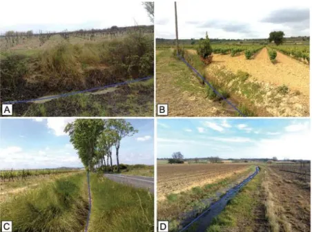
Cultivated landscapes are characterized by linear elements, such as roads, hedgerows, embankments, and ditches (Hirt, Mewes, & Meyer, 2011). These man-made linear features can greatly extend and modify drainage networks (Duke, Kienzle, Johnson, & Byrne, 2006; Wemple, Jones, & Grant, 1996). Man-made drainage networks are particu- larly common in every agricultural landscapes, such as temperate and boreal landscapes (Carluer & Marsily, 2004; Dunn & Mackay, 1996; Herzon & Helenius, 2008; Procopio & Bunnell, 2008), tropical landscapes (Gardner & Gerrard, 2003), and Mediterranean land- scapes (Moussa, Voltz, & Andrieux, 2002; Pita, Mira, & Beja, 2006; Ramos & Porta, 1997; Roose and Sabir, 2002; Warner, 2006) (Figure 1).
These man-made drainage networks impact runoff and groundwater dynamics (Buchanan, Falbo, Schneider, Easton, & Walter, 2012; Carluer & Marsily, 2004; Dages et al., 2009; Moussa et al., 2002) and also erosional processes (Gardner & Gerrard 2003; Paroissien, Lagacherie, & Le Bissonnais, 2010; Ramos & Porta 1997). Often associated with terrace fronts, these networks thus contribute to the stability of terraced hillslopes in Mediterranean areas (Stanchi, Freppaz, Agnelli, Reinsch, & Zanini 2012). As interstitial elements in intensively cultivated landscapes, they may have a significant value in
Figure 1. Four examples of man-made drainage features in the Hérault département in the south of France. (A) a small ditch conveying runoff at the bottom of a terrace front on a hilly landscape, (B) a ditch in a flat area, (C) a roadside ditch and (D) a sunken path that also acts as a drainage ditch.
ecology (Stoate et al., 2009), but this depends on their management. They may provide valuable habitats, enhance connectivity within the landscape and/or harbor rare species (Herzon & Helenius 2008; Mazerolle, 2005; Pita, Mira, & Beja, 2006).
The same way as for the natural drainage networks (Gregory & Walling, 1968; Post & Jakeman, 1996), the man-made drainage density, i.e., the density of man-made drainage networks, has been shown to be a key factor influencing the control of these aforemen- tioned physical processes (Dunn & Mackay, 1996; Finke, Brus, Bierkens, Hoogland, Knotters, & de Vries, 2004; Krause, Jacobs, & Brorstert, 2007). Man-made drainage density seems to be a key parameter especially for controlling surface runoff (Levavasseur, Bailly, Legacherie, Calin, & Robotin, 2012) and the associated soil erosion. Moreover, man-made drainage networks are often dense enough to significantly increase the hydrological connectivity of a catchment. These man-made linear features are thus important to consider when studying the runoff and erosion processes of small, cultivated catchments.
Some studies revealed that man-made drainage densities can be highly variable in space (Lagacherie et al., 2006; Procopio & Bunnell 2008). Modifying the density of these networks could thus be a way to modulate runoff and erosion processes in agricultural landscapes and to modify ecological habitats. However, we need to know how this density is variable in space and the extent to which it depends on the physical landscape before being able to propose some modifications of this density.
Methods for modeling the variability of man-made drainage density that rely on correlations with auxiliary data can be proposed. Such methods are commonly used for digital soil mapping and other environmental sciences applications. According to the methodology proposed by Hengl (2009), methods that combine regressions and
geostatistical modeling can be used to model and estimate drainage densities, depending on whether the drainage density exhibits a spatial structure.
The main objective of this study was to model the spatial variability of man-made drainage density in agricultural landscapes, to understand its variability and the extent to which it depends on the landscapes attributes. We only focused on open-channel drainage and not on tile drainage. This approach included the prior determination of the optimal resolution at which the drainage density was computed. We then used statistical regres- sions from auxiliary environmental data and geostatistical models that exploited spatial structures. Finally, we validated our results using a cross-validation process.
2. Study area
2.1. General description
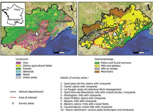
The study area is the cultivated portion of the Hérault French département of the Languedoc-Roussillon région, in the south of France. We did not consider the northern mountainous region, where cultivation is limited, or the eastern part, where urbanization is high (Figure 2). At the département scale, the land-cover is mainly vineyards, comprising 50% of the utilized agricultural area. However, a third of the vineyards have been abandoned for twenty years because of the wine crisis (Direction Départementale des Territoires et de la Mer de l’Hérault, 2011). Nearly 10% of the utilized agricultural area is planted with cereal fields. In the southern and western cultivated areas of the département that we studied, the proportion of vineyards is even higher (approximately 75%). In 2000,
Figure 2. Study area: the survey areas (number 1–10) are distributed throughout the vineyards (A) of the Hérault département and the three main cultivated pedo-landscapes (B).
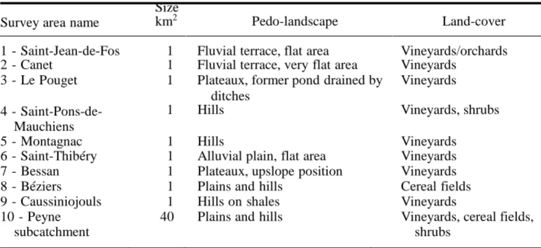
5 - Montagnac 1 Hills Vineyards 6 - Saint-Thibéry 1 Alluvial plain, flat area Vineyards 7 - Bessan 1 Plateaux, upslope position Vineyards 8 - Béziers 1 Plains and hills Cereal fields 9 - Caussiniojouls 1 Hills on shales Vineyards
10 - Peyne 40 Plains and hills Vineyards, cereal fields,
subcatchment shrubs
small farms predominated with an average farm area of 13 ha according to the data from the agricultural census conducted by the Regional Direction of Agriculture and Forest.
The climate is Mediterranean with 600–800 mm of precipitation per year and two short but intense rainy seasons in the autumn and spring. This climate combined with the intensive vine cultivation causes the area to be sensitive to flash flooding and erosion. For example, the mean erosion rate in the study area is 10.5 t ha 1 year 1 but the spatial
variability of the intensity of erosion is high (Paroissien et al., 2010).
The altitude varies between approximately 0 and 350 m in the southern portion of the département. From a geomorphological point of view, we can distinguish four main areas: (1) the alluvial and coastal plains and low terraces of the main rivers, (2) the hilly landscapes that are mostly calcareous but also contain marls (calcareous sedimentary rocks containing a variable amount of clays), (3) the hilly landscapes on shales in the western portion of the area, and (4) the mountains in the northern part of the département (outside of our study area). Two main catchments cover our study area, the catchments of the Hérault and Orb rivers.
2.2. Field data
2.2.1. Spatial sampling of contrasting landscapes located in the study area
All of the man-made drainage networks throughout the entire study area could not be surveyed in the field. Thus, a stratified sampling strategy based on landscape character- istics was performed. The landscape characteristics used to define the sampling strategy were the pedo-landscapes given by soil map 2 (Table 3), the main type of land-cover, and the topography (Figure 2). All of these characteristics were assumed to have an influence on the man-made drainage density of the landscape. Consequently, nine 1 km2 square
areas and one larger area (40 km2 ) were selected (Table 1) for exhaustive field surveys. The goal of selecting the large survey area (the Peyne subcatchment) was to allow us to analyze the spatial variability of drainage densities for multiple scales of analysis.
Table 1. Survey areas characteristics. Survey area name
Size
km2 Pedo-landscape Land-cover 1 - Saint-Jean-de-Fos 1 Fluvial terrace, flat area Vineyards/orchards 2 - Canet 1 Fluvial terrace, very flat area Vineyards 3 - Le Pouget 1 Plateaux, former pond drained by Vineyards 4 - Saint-Pons-de-
Mauchiens
ditches
2.2.2. Data acquisition
In contrast to natural stream networks, man-made drainage networks are almost never mapped on topographical maps. Their remote sensing is not yet accurate enough to create such maps (Bailly, Lagacherie, Millier, Puech, & Kosuth, 2008). Indeed, man-made drainage ditches may be very narrow (widths and depths of less than 1 m) and densely covered with vegetation. Moreover, only features with horizontal dimensions of the same order of magnitude as the ground resolution of remotely sensed data can be detected (Notebaert, Verstraeten, Govers, & Poesen, 2009). This limits the usability of remote sensing at a regional scale, because very high resolution data are not available at this scale (Notebaert et al., 2009). Therefore, drainage density cannot be accurately inferred from the delineations provided by geodatabases or remote sensing data. We thus conducted field surveys of these man-made drainage networks in the spring and summer of 2010 at an average speed of 1.5–3 km2 per day and per person according to the difficulty of the
terrain. The man-made drainage networks mainly consisted of agricultural ditches, road- side ditches, culverts, canalized streams, and sunken paths and roads. The width and depth of these elements varied from approximately 50 cm to several meters. Fifty centimeter aerial photographs were used at a scale of 1:5000 to locate the elements of the drainage networks in the fields. The man-made drainage networks were then digitalized and georeferenced using the Quantum GIS (QGIS) software (Quantum GIS Development Team, 2011).
3. Methods
The methodology of the proposed modeling process includes four steps: (1) the selection of a geographical support to model the drainage density; (2) the selection and calibration of a spatial explanatory model;
(3) the identification of the potential landscape explanatory variables of the man- made drainage density; and
(4) the assessment of the performance of the explanatory model.
3.1. Selecting a geographical support 3.1.1. Square grid-based analysis
To model the drainage density, we used a square grid for which the cumulated length of the drainage network divided by the grid cell area was attributed to each grid cell. This square grid represented the geographical support, i.e., a given spatial arrangement made of geometrical entities.
A grid-based analysis was used for various reasons. Square grids allowed us to model the drainage density throughout the landscape with the same geographical support. This would not be possible if either individual drainage features (e.g., a ditch) or catchments were used as the spatial scale of the analysis. Moreover, a square grid-based analysis allowed us to link the spatial variability of the drainage density with landscape explana- tory variables. We could have used kernel estimators instead, but we chose a square grid- based analysis because of its simplicity and the absence of edge effects. Furthermore, the use of a square grid allowed us to maintain the maximal spatial variability of the drainage densities. For all of these reasons, grid-based analyses have been used in various studies to
compute the densities of linear elements of landscapes, such as streams (Luoto, 2007; Oguchi, 1997), hedgerows (Burel & Baudry, 1990; Deckers, Kerselaers, Gulinck, Muys, & Herny, 2005), roads (Hawbaker, Radeloff, Hammer, & Clayton, 2005), or lineaments (linear features on the Earth’s surface, e.g., faults) (Casas et al., 2000). Nevertheless, the use of a square grid creates an issue with the selection of the grid cell size (Borruso, 2003). To deal with this issue, we proposed a method to define empirically the optimal grid cell size in our study.
3.1.2. Selection of the grid cell size for the spatial modeling of man-made drainage density
Numerous studies have dealt with the selection of the grid cell size (Duveiller & Defourny, 2010; Hengl, 2006; Obeysekera & Rutchey, 1997). However, none of these studies have considered the case of making density maps from maps of linear features, though these studies have considered the use of different criteria to optimize the cell resolution (e.g., object detection in images). Moreover, all of these studies dealt with the case of a variable fully defined in space, such as elevation or land-cover. In studies concerned with the densities of linear features, the selection of the scale was often arbitrary (Hawbaker et al., 2005) or related to farms or fields characteristics (Burel & Baudry 1990; Deckers et al., 2005). Nevertheless, Casas et al. (2000) suggested that the best choice of grid cell size to study the densities of lineaments would be the one that respected the average spacing between the lineament under examination. Using a grid that respects the line spacing allows for the minimization of the number of cells that do not contain any lines.
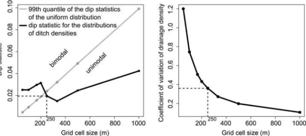
To take into account the line spacing, we proposed to directly determine the grid cell size for which no bimodality in the distribution of the resulting drainage densities was observed. The test for unimodality was performed using the dip-test (Hartigan & Hartigan, 1985) in the GNU-R software (R Development Core Team, 2010). The dip statistics were computed for the drainage density distributions from the samples with grid cell sizes of 50, 100, 166, 200, 250, 333, 500, and 1000 m; each value is approximately a divisor of the size of most of the survey areas (1000 1000 m). The values of the dip statistics were then compared with the values of the dip statistic for 100,000 uniform distributions. We could reject the null hypothesis of unimodality with an error probability of less than 1% (arbitrary threshold) if the dip statistic for the tested sample was higher than the 99th quantile of the distribution of the dip statistics for the uniform distribution.
However, we searched for a coefficient of variation of drainage densities that remained high because we also wanted to maintain a high variability of drainage densities. The best cell size for this study should therefore be a compromise between the line spacing and the variability of the resulting drainage densities.
3.2. Spatial explanatory model of man-made drainage density
To select a spatial explanatory model, Hengl (2009) proposed a general decision tree. Using this framework, we chose a regression-kriging model. Regression-kriging combines a regression of the dependent variable on the auxiliary variables with the simple kriging of the regression residuals (residual kriging). This method allows the user to separately interpret the power of the regression model, the deterministic part, and that of the kriging interpolation, the stochastic part, i.e., the unexplained part of the variability (Hengl, Heuvelink, & Rossitier 2007). An advantage is thus to measure the spatial correlation
in randomness that can drive to consider other processes. Hence, this method has been used in many studies because of its simplicity and its ability to consider both a determi- nistic component and a spatial dependence structure to model a variable, e.g., for the prediction of meteorological data (Alsamamra, Ruiz-Arias, Pozo-Vázquez, & Tovar- Pescador, 2009) or soils properties (Hengl et al., 2007).
For the regression model, we chose a multiple linear regression (MLR) model. From the residuals of the MLR model, we computed an empirical semivariogram (Matheron, 1962), which plots the semivariance, i.e., the expected squared increment of the residuals distant from a given distance h against the distance h. From the empirical semivariogram, a semivariogram was modeled and used for the modeling of the residuals in the unsampled areas by kriging interpolation. Thus, the target variable, i.e., the drainage density, could be expressed for an unsampled location s0 as the sum of the deterministic
and stochastic components Hengl (2009).
^zðs0 Þ ¼ m^ ðs0 Þ þ ^eðs0 Þ (1) p n ^zðs0 Þ ¼ X β^k qk ðs0 Þ þ X λi eðsi Þ (2) k¼0 Pp i¼1
where m^ ðs0 Þ ¼ Pk¼0 β^k qk ðs0 Þ is the fitted deterministic component, i.e., the MLR n
model; ^eðs0 Þ ¼ i¼1 λi eðsi Þ is the interpolated residual; p is the number of explanatory
variables of the MLR model; n is the number of observations; β^k are the estimated MLR
model coefficients (β^0 is the estimated intercept); qk ðs0 Þ are the values of the explanatory
variables at location s0 ; λi are the kriging weights depending on the spatial dependence
structure of the MLR residuals and eðsi Þ is the residual at location si . The MLR
coefficients β^k were estimated from the training sample by the ordinary least squares
(OLS) method.
We used the geoR library in the GNU-R software to perform the regression-kriging.
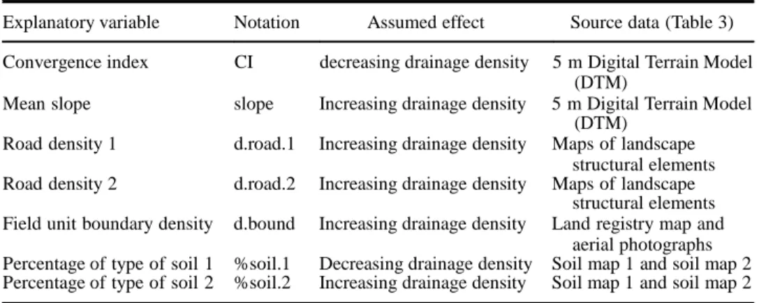
3.3. Identification of potential explanatory variables of man-made drainage densities We included seven potential explanatory variables relative to landscapes attributes to model man-made drainage density, all represented by quantitative variables (Table 2). These variables were the Convergence Index, mean slope, two variables related to road density, the density of field unit boundary and two variables related to soil type.
To identify these explanatory variables, we considered the role of the man-made drainage networks. According to the literature, the roles of man-made drainage networks are the interception of runoff from hillslopes and roads, the lowering of the water table via the drainage of groundwater and the conveyance of water towards downstream areas (Adamiade, 2004; Carluer & Marsily, 2004; Duke et al., 2006; Dunn & Mackay, 1996; Ramos & Porta, 1997).
We first considered the influence of topography on runoff production and accumula- tion. We computed two topographic indices: the convergence index with a search radius of 250 m (Kothe & Lehmeier, 1996) and the slope derived from the 5 m Digital terrain model (DTM) (Table 3). They were both computed using SAGA GIS (http://saga-gis.org). Low values of the convergence index corresponded to areas where water converges; thus, high convergence index values were assumed to indicate a low drainage density.
Table 2. Description of the selected explanatory variables and their assumed effect on the man-made drainage density.
Explanatory variable Notation Assumed effect Source data (Table 3) Convergence index CI decreasing drainage density 5 m Digital Terrain Model
(DTM)
Mean slope slope Increasing drainage density 5 m Digital Terrain Model (DTM)
Road density 1 d.road.1 Increasing drainage density Maps of landscape structural elements Road density 2 d.road.2 Increasing drainage density Maps of landscape
structural elements Field unit boundary density d.bound Increasing drainage density Land registry map and
aerial photographs Percentage of type of soil 1 %soil.1 Decreasing drainage density Soil map 1 and soil map 2 Percentage of type of soil 2 %soil.2 Increasing drainage density Soil map 1 and soil map 2
Table 3. Available spatial data.
Description Year Type Scale/Resolution Producer/owner Aerial photographs
(BD ORTHO®)
2009 Raster 50 cm Institut Géographique National (IGN) Maps of landscape structural
elements (SCAN 25®)
2006 Raster 2.5 m IGN
Digital Terrain Model (DTM) 2005 Raster 5 m Conseil Général de l’Hérault Soil map 1 1993 Vector 1:100,000 Institut National de la
Soil map 2 1999 Vector 1:250,000
Recherche Agronomique (INRA)
INRA
Land registry map of the 1997 Vector 1:2500 Direction Générale des
Peyne subcatchment Impôts (DGI)
The type of soil in an area affects the runoff production and the possibility of waterlogging. Hence, we classified the different soil units based on three characteristics. Type 1 soils limited the production of runoff and were thus assumed to disfavor high man- made drainage densities. Type 2 soils favored waterlogging and were thus assumed to favor high man-made drainage densities. Type 3 soils had no particular impact on runoff and were assumed to be neutral concerning their impact on man-made drainage density. Many parameters control the soil infiltration capacity (Paré, 2011; Wassenaar, Andrieux, Baret, & Robbez-Masson, 2005) and consequently the production of Hortonian runoff which is the prevalent runoff in Mediterranean areas. The effect of soil tillage or the amount of grass cover, for instance, can be very important in reducing runoff, but these factors are not constant in time and thus not easy enough to map to be considered here. However, the presence of stones on the surface was also recognized as a key parameter that can increase the soil infiltration capacity (Poesen, Ingelmo-Sanchez, & Mucher, 1990; Wassenaar et al., 2005). In our study, the soils with numerous and not embedded stones on the surface were thus classified as type 1 soils. For instance, the soils of the Bessan, Caussiniojouls, and Saint-Jean-de-Fos survey areas were considered to be type 1 soils, as well as some parts of the Peyne, Saint-Thibéry, and Canet areas. Concerning
waterlogging, the soils that had a deep heavy, horizon were classified as type 2 soils; the best example of this was the soils of the survey area of Montagnac. These soils were also present on parts of the Saint-Pons-de-Mauchiens area. All the other types of soils were classified as type 3. Thus, the two explanatory variables selected concerning soil type were the percentage of type 1 soils and the percentage of type 2 soils within a grid cell.
To take into account the impacts of roadside ditches, two explanatory variables were chosen: the density of the main and secondary roads (d.roads.1) considered to be regularly maintained on the Institut Géographique National (IGN) maps (Table 3) and the density of other roads (d.roads.2) also considered to be regularly maintained but of lesser importance. The roads were digitized on the maps of the landscapes structural elements (Table 3).
The density of field unit boundaries was added as another possible explanatory variable of man-made drainage density. Agricultural ditches were the most frequent features of these networks and were always located along field unit boundaries. For instance, we surveyed a few agricultural ditches in the Béziers area which is covered by large cereal fields.
Natural areas were not considered in our study, although they certainly decreased surface runoff. First, few natural areas were present in our survey areas (except in Saint- Pons-de-Mauchiens). Second, when a large patch of natural area was present, the density of the field unit boundaries accounted for the expected effect of the decreased drainage density caused by the presence of natural areas because we considered only boundaries of cultivated field units.
These explanatory variables may be considered orthogonal (maximum coefficient of correlation ρ ¼ 0:25). We gathered various maps (Table 3) to compute these variables. Two soil maps were needed because the most detailed soil map did not cover the entire study area.
3.4. Assessment of the performances of the explanatory model
We assessed the performances of the multiple linear regression alone and multiple linear regression coupled with residual kriging. We used V-fold cross-validation with a hundred repetitions. The sample was randomly divided into ten different sub-samples. Nine sub- samples were used for training, i.e., for calibrating the multiple linear regression and for estimating the semivariogram parameters of the residuals. The tenth was used for valida- tion: the drainage density was modeled by using the multiple linear regression calibrated on the nine sub-samples, alone or coupled with residual kriging. We first repeated this operation ten times by changing the validation sub-sample each time, and we then repeated these ten operations a hundred times by changing the random division of the sample to avoid any sampling effects in the results. To assess the performances of the spatial model, we analyzed the distribution of the coefficient of determination (R2 ) and the
root mean squared error (RMSE) in both the training samples and the validation samples. Then, we analyzed the estimates of the regression coefficients to compare the effect of each explanatory variable.
4. Results
4.1. Selection of the grid cell size for the spatial modeling of man-made drainage density
We could reject the null hypothesis of unimodality with an error probability of less than 1% for a cell size inferior to 250 m (Figure 3, left). Thus, 250 m was the minimum cell
Figure 3. Selection of the grid cell size. Left: dip statistics of the unimodality test as a function of the grid cell size. Right: coefficient of variation of drainage density as a function of the grid cell size.
size considered. The coefficient of variation of the drainage densities decreased exponen- tially with the grid cell size (Figure 3, right); therefore, we chose the minimum grid cell size of 250 m to maintain the maximum variability.
We took six grid cells in the Peyne subcatchment as an example of the drainage density computation with a cell size of 250 m (Figure 4). There was a clear difference in drainage density between the northwestern cell where the drainage density was higher than 200 m ha 1 in comparison with the southeastern cells where the density was near
zero (there were almost no man-made drainage networks present). Finally, with a grid cell size of 250 250 m, we obtained a total of six hundred and sixty three grid cells: sixteen
Figure 4. Example of the computation of the drainage density of six contrasted grid cells in the Peyne subcatchment at a resolution of 250 250 m.
grid cells for each of the nine survey areas of 1 km2 (which represented a hundred and
forty four grid cells) and five hundred and nineteen grid cells for the Peyne subcatchment. The equivalent grid cell area was 62,500 m2 . This cell area was much greater than the
average field unit area (6500 m2 ) in our survey areas.
4.2. Variability of drainage densities among and inside survey areas
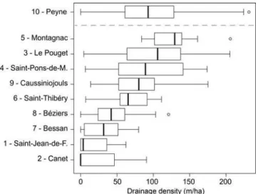
The ten survey areas exhibited a large amount of variability in man-made drainage density (Figure 5). The survey area with the lowest median drainage density was Canet, a very flat area on the terrace of the Hérault River. The other survey areas in plains also had low median drainage densities (Saint-Jean-de-Fos, Béziers, Saint-Thibéry), as did as the survey area of Bessan, which was expected due to its particularly well-drained soil and its upslope location in the landscape. The hilly landscapes had higher median drainage densities, with a maximum median drainage density equal to 129 m ha 1 for Montagnac.
For all of the survey areas, the minimal drainage density was less than 10 m ha 1 , except
for Caussiniojouls (14 m ha 1 ) and Montagnac (84 m ha 1 ). The maximum drainage
density was greater than 200 m ha 1 for Le Pouget (205 m ha 1 ), Montagnac (206 m
ha 1 ) and the Peyne subcatchment (231 m ha 1 ).
We also noticed a high variability in the drainage densities within each survey area (Figure 5). This finding is especially true for Caussiniojouls, Saint-Pons-de-Mauchiens, Le Pouget, and the Peyne survey areas, with ranges in drainage density equal to 161, 167, 201, and 231 m ha 1 , respectively. However, in the case of the Peyne subcatchment, the
number of cells was much greater (five hundred and nineteen grid cells versus sixteen for each of the other nine survey areas). Thus, we had to explain two kinds of variability: the variability among survey areas and the variability inside each survey area. Finally, this high spatial variability in man-made drainage density reinforced the interest in modeling man-made drainage densities.
Figure 5. Distributions of drainage density by survey area. All of the plots represent 16 grid cells of 250 250 m, except for the Peyne subcatchment (519 grid cells). The line within the box represents the median, while the boxes represent the interquartile range, and the whiskers extend to the most extreme data point which is no more than 1.5 times the interquartile range from the box.
4.3. Spatial modeling of drainage densities
4.3.1. Results of the multiple linear regression (MLR) model
4.3.1.1. Performances of the MLR model. We first verified the hypothesis of the linear model. The normality of the residuals of the model was confirmed with a Shapiro test. No heteroskedasticity (heterogeneity of the variance of the residuals) was observed for the residuals.
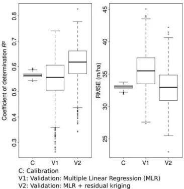
The distributions of the coefficient of determination (R2 ) were computed for the
training sample and for the validation sample, as well as the distributions of the RMSE (Figure 6). The median R2 indicated that the MLR model explained 55% of the
variability in the validation sample. Moreover, three-quarters of the validation samples produced an R2 between 0.51 and 0.61. The median error was almost zero in the
validation sample (6 10 3 m ha 1 ). The median RMSE for the validation samples was 36 m ha 1 (33 m ha 1 for the training sample), which represented 41% of the
mean drainage density. Finally, no significant effect of over-fitting was observed for the training sample, which had a median adjusted R2 of 0.560 in comparison to the median
R2 of 0.565.
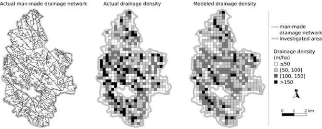
We compared the maps of the actual and modeled drainage densities with the MLR model for the Peyne subcatchment (Figure 7). Our model allowed to distinguish between areas with high drainage densities and areas with low drainage densities. The pattern of the variation in the drainage density was well simulated. However, the modeled map appeared more smoothed than the actual map.
Figure 6. Model quality. Left: coefficient of determination. Right: root mean squared error. The line within the box represents the median, while the boxes represent the interquartile range, and the whiskers extend to the most extreme data point which is no more than 1.5 times the interquartile
Figure 7. Maps of man-made drainage networks and of the actual and the modeled man-made drainage densities for the Peyne subcatchment.
4.3.1.2. Importance of each explanatory variable. Before analyzing the estimations of the regression coefficients, we first verified that the estimations of the regression coeffi- cients were not too dependent on the training sample. For this purpose, we assessed the variability in the estimates of the regression coefficients following the cross-validation process. The coefficients of variation of the coefficient estimates of the cross-validation process were lower than 10%. Therefore, we used the model calibrated on the entire sample to analyze the importance of each explanatory variable.
Table 4 presents the importance of each explanatory variable. First, all the variables were considered highly significant (all with p-values of t-tests less than 0.001). The expected effects were verified for all the variables: the slope, road density 1, road density 2, the percentage of type 2 soils, and the density of field unit boundaries increased the drainage density, whereas the convergence index and the percentage of type 1 soils decreased the drainage density.
When looking at the standardized regression coefficients (Table 4), the most influen- tial variables in decreasing order were: the convergence index, road density 1, the slope (or rather the log of slope), the percentage of type 1 soils, the field unit boundary density (or rather its log), road density 2, and percentage of type 2 soils.
According to the relative importance of each explanatory variable, we built new multiple linear regression models by progressively adding a variable at each step in
Table 4. Results of the multiple linear regression. Variable Estimate
Standard
deviation Standardized regression coefficient p-value Intercept (k) 71.56 22.36 1 10 3 CI −1.632 0.09671 −0.4506 2 10 53 log(slope) 20.70 2.171 0.2523 3 10 20 d.road.1 1.305 0.08222 0.4199 3 10 48 d.road.2 0.3672 0.06111 0.1625 3 10 9 %soil.1 −0.3765 0.03983 −0.2513 6 10 20 %soil.2 0.3540 0.09291 0.09915 1 10 4 log(d.bound) 23.33 3.578 0.1739 1 10 10
Table 5. Results of the partial multiple linear regression models.
Model Adjusted R2 Additional variability
explained % k+CI 0.21 21 k+CI+d.roads.1 0.34 13 k+CI+d.roads.1+log(slope) 0.42 8 k+CI+d.roads.1+log(slope)+%soil.1 0.48 6 k+CI+d.roads.1+log(slope)+%soil.1+d.bound 0.53 4 k+CI+d.roads.1+log(slope)+%soil.1+d.bound+d.roads.2 0.55 3 k+CI+d.roads.1+log(slope)+%soil.1+d.bound+d.roads.2+% soil.2 0.56 1
order of importance (Table 5). Two variables increased the amount of variability in drainage density explained by the model by more than 10% (the convergence index and the density of roads 1). Two others variables caused a 5% increase or greater (the log of slope and the percentage of type 1 soils), and the last three variables only resulted in a 4%, 3% and 1% increase, for the density of field unit boundaries, the density of roads 2 and the percentage of type 2 soils, respectively.
4.3.2. Results of the regression-kriging model
4.3.2.1. Variogram of the residuals of the MLR model. We looked at the variogram of the residuals of the MLR model computed using the entire sample (Figure 8). The spatial structure was low. Indeed, the nugget effect was predominant, and the spatial structure was only significant from 250 to 500 m. We could thus hypothesize that the improvement brought by residual kriging would be limited.
4.3.2.2. Performances of the regression-kriging model. When adding residual kriging to the multiple linear regression results, the median R2 was equal to 61%, which represented an improvement of 6% in comparison with the MLR model alone (Figure 6). Three- quarters of the validation samples produced an R2 between 0.57 and 0.66. The median
error was still almost zero (0.02 m ha 1 ), and the RMSE was 33 m ha 1 , which
Figure 8. Semivariogram of the residuals of the multiple linear regression model for the entire sample.
represented 38% of the mean drainage density. The regression-kriging model was thus able to explain more than half of the variability in the man-made drainage density, but the deterministic part of the model was able to better explain this variability than the stochastic part (residual kriging).
5. Discussion
5.1. Variability and explanation of the man-made drainage density throughout agricultural landscapes
Man-made drainage networks were ubiquitous in the surveyed Mediterranean vineyard landscapes of the Hérault département. The drainage density modeling at an optimized grid cell size revealed a high variability in the man-made drainage density. This variability was observed at two scales, among the survey areas (greater than or equal to 1 km2 ) and
inside each survey area (less than 1 km2 ). The man-made drainage densities varied from 0
to 231 m ha 1 at the selected resolution of 250 × 250 m. This variability was successfully
explained by seven easily available explanatory variables and residual kriging, with 61% of the variability explained and a RMSE of 33 m ha 1 . Therefore, the model results
allowed us to distinguish between areas with high drainage densities and areas with low drainage densities.
Moreover, our model was also able to explain much more variability in man-made drainage density than drainage density computed from usual hydrographic databases. Indeed, the percentages of explained variability (i.e., the coefficient of determination) with the drainage density extracted from hydrographic databases (BD TOPO, BD Carthage, Institut Géographique National) was equal to 14% for the cell size of 250 m. Moreover, we noticed that only 22% of the network length surveyed in the fields were represented in the hydrographic databases, and this percentage varied greatly (between 0% and 77%) depending on the survey area. We also tried to explain the drainage density with the density of channels extracted from Digital Terrain Models. We used the classical D8-algorithm (O’Callaghan and Mark, 1984) with a 5 m DTM and various initiation thresholds (from 1000 m2 to 500,000 m2 ). Regardless of the initiation
threshold, the amount of variability explained was very low in comparison with our model, from 0% to 15%.
5.2. Spatial explanatory model
Regression-kriging explained 61% of the variability of the man-made drainage den- sities. Multiple linear regression was able to explain most of this variability without residual kriging. Residual kriging only increased the amount of variability explained by 6%. Moreover, this improvement by residual kriging was mainly virtual because it relied on a sampling strategy of 90%. However, according to the semivariogram of the residuals of the MLR model, in which the range was less than 750 m, a dense sampling strategy was compulsory to consider the low spatial dependence structure of the residuals.
One of the interesting aspects of regression - kriging is its ability to consider explanatory models other than linear regression (Hengl et al., 2007). Hence, we also tested regression trees, which provided similar performances, but we selected MLR because we found it easier to interpret.
5.3. Discussion of the effect of each explanatory variable
The topography and the soil type were found to be important explanatory variables of the man-made drainage density. The areas where water converged were found to favor higher drainage densities, as well as steep areas where runoff could cause greater soil loss without ditches. In fact, the convergence index was found to be the most important parameter for modeling the man-made drainage density. The type of soil modulated the effect of topography: soils with high stone contents (type 1 soils) disfavored surface runoff and high drainage densities, whereas soils with a deep heavy horizon (type 2 soil) favored water-logging and high drainage densities. Nevertheless, the importance of the percentage of type 2 soils was very limited (explaining only an additional 1% of the variability in drainage density). This result could be explained by the fact that this type of soil occurred in only a few grid cells (only fifteen, mainly in Montagnac). If we had sampled more in areas with this type of soil, this variable would have likely been more significant.
The density of roads explained the high number of roadside ditches and was thus one of the most important explanatory variables (the density of primary and secondary roads). Furthermore, a clear distinction was made between main and secondary roads, which were often bordered by ditches on both sides (1.31 m of ditch for every 1 m of roads), and other roads, which were not necessary bordered by ditches (0.37 m of ditch for every 1 m of roads). The density of trails or pathways (computed from IGN maps) was also tested as an explanatory variable, without success.
The last variable, the density of field unit boundaries (related to the mean field unit area), explained only a small amount of the variability in the drainage density. This result is in contrast with studies on the density of hedgerows (Kantelhardt, Osinski, & Heissenhuber, 2003). Except for rare areas where the field units were very large (which explained the low drainage density), field units were small- to medium-sized in the majority of the areas and corresponded to contrasted situations of drainage densities. For instance, if no land consolidation had occurred in the past, the field units may have remained small in areas where man-made drainage was not useful (flat area or at the top of a hill-slope, for instance). Land consolidation was indeed limited in the study area. However, farmers also maintained small field units because the removal of field unit boundaries and their associated man-made drainage networks would have increased the amounts of surface runoff and soil loss. In fact, we met some farmers who claimed to have preserved a boundary and its associated ditch between two of their field units to limit surface runoff.
5.4. Transferability of the methodology
The methodology presented in this paper is transferable to other study areas. The selection of the grid cell size should be adapted to the data, by using the method proposed here. The regression-kriging model can be applied for any data set of drainage densities and explanatory variables relative to landscape attributes. Concerning the explanatory vari- ables, they were all selected according to the hypothesized hydrological functioning of cultivated landscapes. These variables should thus be relevant in any study area, even if the estimated coefficients would obviously vary. For example, whether the ditches are mainly created to limit soil erosion (Ramos & Porta, 1997) or to drain groundwater (Finke et al., 2004; Krause et al., 2007) should have an impact on the coefficients estimates. Different climate, soils, and agricultural history should thus be taken into account. Finally,
in addition to the variables chosen in this study, any other explanatory variables could be integrated in the regression kriging model according to the local knowledge of the study area.
5.5. Where did the unexplained variability come from? 5.5.1. Inappropriate explanatory variables
First, it is possible that several determinants were poorly mapped by our selected explanatory variables. For instance, accounting for the role of soil in modulating the drainage density was strongly hampered by the precision of the available soil maps. The lack of a better consideration of soil data could possibly explain why the Saint-Jean-de- Fos area was poorly modeled, as the soils in this area were very stony in comparison with those in other survey areas. Directly considering the sensitivity of soils to erosion could allow to better account for the role of ditches in preventing soil erosion in Mediterranean areas (Ramos & Porta, 1997; Stanchi et al., 2012) and finally to better model man-made drainage density. The global morphology was also perhaps poorly considered. For example, the Saint-Jean-de-Fos and Canet areas were located in very wide and flat valleys and exhibited very low drainage densities, which was not reflected in our local topo- graphic indices. We tried, however, to take into account the topography at various scales without success. For example, we tested the multi resolution valley bottom flatness index (Gallant & Dowling, 2003), which allows to discriminate valleys at multiple scales, as an explanatory variable.
5.5.2. Unmapped determinants
In parallel with studies conducted on the density of hedgerow networks (Kantelhardt et al., 2003; Llausà, Ribas, Varga, & Vila, 2009; Thenail, 2002), we hypothesized that some technoeconomic factors, such as the productivity, the technical means, and the quality approach of the farms could certainly explain why farmers choose whether or not to preserve man-made drainage networks. However, we were unable to map these potential determinants by adapted explanatory variables in our area at our study scale.
Another driver that was also not thoroughly considered was the presence of tile drainage in field units. Indeed, tile drainage was necessarily associated with a ditch to convey the drained water. Tile drainage was used mainly in areas of water convergence and where soils favored waterlogging, and thus, the convergence index and the percentage of type of soil 2 partly considered tile drainage. Nevertheless, the topography was not the only driver of tile drainage, as there were other factors that depended on the farms and on the farmers’ individual decisions. Interactions between surface drainage and tile drainage could thus be taken into account. For example, Hirt, Meyer, and Hammann, (2005) proposed a method to map the proportion of tile drainage areas for a large catchment. Tile drainage was however limited in our study area: less than 5% of the field units were tile drained according to the data from the agricultural census conducted by the Regional Direction of Agriculture and Forest. Therefore, not taking tile drainage into account should not impact a lot our results.
In the Béziers area, where the man-made drainage densities were low and the land was formerly used as vineyards but almost entirely covered by cereal fields in 2010, we hypothesized that farmers no longer preserved man-made drainage networks and that
these networks had been filled in by soil tillage. To test this hypothesis, another area that is newly cultivated with cereals should be surveyed.
The current man-made drainage networks are the result of individual farmers’ deci- sions to dig a ditch and to various more global drainage policies (like in Le Pouget area) during the last two thousand years (Berger, 2000) and are presently still evolving. During our field surveys, we noticed some new ditches being dug while others were being removed. We also surveyed ditches in areas where vineyards were uncultivated and shrubs were growing; these ditches will most likely disappear in the next few years without further management. Thus, there was some degree of randomness in the man-made drainage density we observed that we could not hope to explain.
Finally, we assumed that these unmapped determinants represent technoeconomic factors which account for the main part of variability not explained by our model. This assumption was reinforced by the almost absence of spatial structure in the residuals of the MLR model. This part of the variability illustrates that man-made drainage density does not depend only on the landscape attributes. Therefore, there remains some latitude to modify the man-made drainage networks. Encouraging farmers to increase or decrease locally the density of these man-made drainage networks, according to the objective of the catchment managers, could thus help to modulate erosion and hydrological processes.
6. Conclusion
This study revealed that the man-made drainage density was not well modeled by the natural drainage density computed from hydrographic databases. We then built an expla- natory model of man-made drainage density by incorporating explanatory variables relative to landscape attributes. This model explained the main part of the variability in the man-made drainage density. Some technoeconomic factors should be tested in the future to understand the part of variability not explained by landscapes attributes. This study thus revealed the extent to which man-made drainage density depends on landscape attributes and that latitude remains for catchment managers in order to modify these networks and preventing soil erosion or flash floods. This modeling approach could also have applications in hydrology or ecology, by providing a spatial estimation of the man- made drainage density which can be an important parameter in hydrological or ecological models.
Acknowledgments
This work was partly supported by the French Languedoc-Roussillon région, via a PhD thesis grant. Field surveys were partly realized within the framework of the CNES-ORFEO program. The authors also thank Adeline Bellet, an MSc student, who helped with the field surveys.
References
Adamiade, V. (2004). Inuence d`un fossé sur les écoulements rapides au sein d`un versant. Paris: Université Pierre et Marie Curie.
Alsamamra, H., Ruiz-Arias, J. A., Pozo-Vázquez, D., & Tovar-Pescador, J. (2009). A comparative study of ordinary and residual kriging techniques for mapping global solar radiation over southern Spain. Agricultural and Forest Meteorology, 149(8), 1343–1357.
Bailly, J. S., Lagacherie, P., Millier, C., Puech, C., & Kosuth, P. (2008). Agrarian landscapes linear features detection from LiDAR: Application to artificial drainage networks. International Journal of Remote Sensing, 29(12), 3489–3508.
Berger, J. (2000). Les fossés bordiers historiques et l’histoire agraire rhodanienne. Etudes Rurales, 153–154, 59–90.
Borruso, G. (2003). Network density and the delimitation of Urban Areas. Transactions in GIS, 7(2), 177–191.
Buchanan, B. P., Falbo, K., Schneider, R. L., Easton, Z. M., & Walter, M. T. (2012). Hydrological impact of roadside ditches in an agricultural watershed in Central New York: Implications for non-point source pollutant transport. Hydrological Processes, 27, 2422–2437.
Burel, F., & Baudry, J. (1990). Structural dynamic of a hedgerow network landscape in Brittany France. Landscape Ecology, 4(4), 197–210.
Carluer, N., & Marsily, G. D. (2004). Assessment and modelling of the influence of man-made networks on the hydrology of a small watershed: Implications for fast flow components, water quality and landscape management. Journal of Hydrology, 285(1–4), 76–95.
Casas, A. M., Cortés, A. L., Maestro, A., Soriano, M. A., Riaguas, A., & Bernal, J. (2000). LINDENS: A program for lineament length and density analysis. Computers & Geosciences, 26(9–10), 1011–1022.
Dages, C., Voltz, M., Bsaibes, A., Prévot, L., Huttel, O., Louchart, X., … Negro, S. (2009). Estimating the role of a ditch network in groundwater recharge in a Mediterranean catchment using a water balance approach. Journal of Hydrology, 375(3–4), 498–512.
Deckers, B., Kerselaers, E., Gulinck, H., Muys, B., & Hermy, M. (2005). Long-term spatio-temporal dynamics of a hedgerow network landscape in Flanders, Belgium. Environmental Conservation, 32(1), 20–29.
Direction Départementale des Territoires et de la Mer de l’Hérault (2011). Regard sur l’Hérault -l’Agriculture (Technical report). Montpellier: DDTM 34.
Duke, G. D., Kienzle, S. W., Johnson, D. L., & Byrne, J. M. (2006). Incorporating ancillary data to refine anthropogenically modified overland flow paths. Hydrological Processes, 20(8), 1827– 1843.
Dunn, S. M., & Mackay, R. (1996). Modelling the hydrological impacts of open ditch drainage. Journal of Hydrology, 179(1–4), 37–66.
Duveiller, G., & Defourny, P. (2010). A conceptual framework to define the spatial resolution requirements for agricultural monitoring using remote sensing. Remote Sensing of Environment, 114, 2637–2650.
Finke, P., Brus, D., Bierkens, M., Hoogland, T., Knotters, M., & de Vries, F. (2004). Mapping groundwater dynamics using multiple sources of exhaustive high resolution data. Geoderma, 123(12), 23–39.
Gallant, J. C., & Dowling, T. I. (2003). A multiresolution index of valley bottom flatness for mapping depositional areas. Water Resources Research, 39(12), 1347–1359.
Gardner, R. A. M., & Gerrard, A. J. (2003). Runoff and soil erosion on cultivated rainfed terraces in the Middle Hills of Nepal. Applied Geography, 23(1), 23–45.
Gregory, K. J., & Walling, D. E. (1968). The variation of drainage density within a catchment. International Association of Scientific Hydrology. Bulletin, 13, 61–68.
Hartigan, J. A., & Hartigan, P. M. (1985). The dip test of unimodality. The Annals of Statistics, 13 (1), 70–84.
Hawbaker, T., Radeloff, V., Hammer, R., & Clayton, M. (2005). Road density and landscape pattern in relation to housing density, and ownership, land cover, and soils. Landscape Ecology, 20(5), 609–625.
Hengl, T. (2006). Finding the right pixel size. Computers & Geosciences, 32(9), 1283–1298. Hengl, T. (2009). A practical guide to geostatistical mapping of environmental variables (2nd ed.).
Luxembourg: European Communities.
Hengl, T., Heuvelink, G. B., & Rossiter, D. G. (2007). About regression-kriging: From equations to case studies. Computers & Geosciences, 33(10), 1301–1315.
Herzon, I., & Helenius, J. (2008). Agricultural drainage ditches, their biological importance and functioning. Biological Conservation, 141(5), 1171–1183.
Hirt, U., Mewes, M., & Meyer, B. C. (2011). A new approach to comprehensive quantification of linear landscape elements using biotope types on a regional scale. Physics and Chemistry of the Earth, Parts A/B/C, 36(12), 579–590.
Hirt, U., Meyer, B. C., & Hammann, T. (2005). Proportions of subsurface drainages in large areas methodological study in the Middle Mulde catchment (Germany). Journal of Plant Nutrition and Soil Science, 168(3), 375–385.
Kantelhardt, J., Osinski, E., & Heissenhuber, A. (2003). Is there a reliable correlation between hedgerow density and agricultural site conditions? Agriculture, Ecosystems & Environment, 98 (1–3), 517–527.
Kothe, R., & Lehmeier, F. (1996). SARA - system zur automatischen relief-analyse. Benutzerhandbuch: Department of Geography, University of Gttingen.
Krause, S., Jacobs, J., & Bronstert, A. (2007). Modelling the impacts of land-use and drainage density on the water balance of a lowland-floodplain landscape in northeast Germany. Ecological Modelling, 200(3–4), 475–492.
Lagacherie, P., Diot, O., Domange, N., Gouy, V., Floure, C., Kao, C., … Szleper, V. (2006). An indicator approach for describing the spatial variability of artificial stream networks with regard to herbicide pollution in cultivated watersheds. Ecological Indicators, 6(2), 265–279.
Levavasseur, F., Bailly, J., Lagacherie, P., Colin, F., & Rabotin, M. (2012). Simulating the effects of spatial configurations of agricultural ditch drainage networks on surface runoff from agricultural catchments. Hydrological Processes, 26, 3393–3404.
Llausàs, A., Ribas, A., Varga, D., & Vila, J. (2009). The evolution of agrarian practices and its effects on the structure of enclosure landscapes in the Alt Empordà (Catalonia, Spain), 1957– 2001. Agriculture, Ecosystems & Environment, 129(1–3), 73–82.
Luoto, M. (2007). New insights into factors controlling drainage density in subarctic landscapes. Arctic, Antarctic, and Alpine Research, 39(1), 117–126.
Matheron, G. (1962). Traité de Géostatistique appliquée (Tome 1). ed. Paris: Editions Technip. Mazerolle, M. (2005). Drainage ditches facilitate frog movements in a hostile landscape. Landscape
Ecology, 20, 579–590.
Moussa, R., Voltz, M., & Andrieux, P. (2002). Effects of the spatial organization of agricultural management on the hydrological behaviour of a farmed catchment during flood events. Hydrological Processes, 16(2), 393–412.
Notebaert, B., Verstraeten, G., Govers, G., & Poesen, J. (2009). Qualitative and quantitative applications of LiDAR imagery in fluvial geomorphology. Earth Surface Processes and Landforms, 34(2), 217–231.
Obeysekera, J., & Rutchey, K. (1997). Selection of scale for Everglades landscape models. Landscape Ecology, 12, 7–18.
O’Callaghan, J. F., & Mark, D. M. (1984). The extraction of drainage networks from digital elevation data. Computer Vision, Graphics, and Image Processing, 28(3), 323–344.
Oguchi, T. (1997). Drainage density and relative relief in humid steep mountains with frequent slope failure. Earth Surface Processes and Landforms, 22(2), 107–120.
Paré, N. (2011). Pollution de l’eau par les pesticides en milieu viticole languedocien. Construction d’un modèle couplé pression-impact pour l’expérimentation virtuelle de pratiques culturales à l’échelle de petits bassins versants. Montpellier: Montpellier SupAgro.
Paroissien, J., Lagacherie, P., & Le Bissonnais, Y. (2010). A regional-scale study of multi-decennial erosion of vineyard fields using vine-stock unearthing-burying measurements. CATENA, 82(3), 159–168.
Pita, R., Mira, A., & Beja, P. (2006). Conserving the Cabrera vole, Microtus cabrerae, in intensively used Mediterranean landscapes. Agriculture, Ecosystems & Environment, 115(1–4), 1–5. Poesen, J., Ingelmo-Sanchez, F., & Mucher, H. (1990). The hydrological response of soil surfaces to
rainfall as affected by cover and position of rock fragments in the top layer. Earth Surface Processes and Landforms, 15(7), 653–671.
Post, D. A., & Jakeman, A. J. (1996). Relationships between catchment attributes and hydrological response characteristics in small Australian Mountain Ash catchments. Hydrological Processes, 10(6), 877–892.
Procopio, N. A., & Bunnell, J. F. (2008). Stream and wetland landscape patterns in watersheds with different cranberry agriculture histories, Southern New Jersey, USA. Landscape Ecology, 23, 771–786.
Quantum GIS Development Team. (2011). Quantum GIS Geographic Information System. Beaverton, OR: Open Source Geospatial Foundation Project.
R Development Core Team. (2010). R: A language and environment for statistical computing. Vienna: R Foundation for Statistical Computing. ISBN 3-900051-07-0. Retrieved from http:// www.R-project.org
Ramos, M. C., & Porta, J. (1997). Analysis of design criteria for vineyard terraces in the Mediterranean area of North East Spain. Soil Technology, 10(2), 155–166.
Roose, E., & Sabir, M. (2002). Stratégies traditionnelles de conservation de leau et des sols dans le bassin méditerranéen: Classification en vue dun usage renouvellé. Bulletin - Réeseau Erosion, 21, 33–44.
Stanchi, S., Freppaz, M., Agnelli, A., Reinsch, T., & Zanini, E. (2012). Properties, best management practices and conservation of terraced soils in Southern Europe (from Mediterranean areas to the Alps): A review. Quaternary International, 265, 90–100.
Stoate, C., Bldi, A., Beja, P., Boatman, N., Herzon, I., van Doorn, A., … Ramwell, C. (2009). Ecological impacts of early 21st century agricultural change in Europe: A review. Journal of Environmental Management, 91(1), 22–46.
Thenail, C. (2002). Relationships between farm characteristics and the variation of the density of hedgerows at the level of a micro-region of bocage landscape. Study Case in Brittany, France. Agricultural Systems, 71(3), 207–230.
Warner, R. F. (2006). Natural and artificial linkages and discontinuities in a Mediterranean land- scape: Some case studies from the Durance Valley, France. CATENA, 66(3), 236–250. Wassenaar, T., & Arieux, P., Baret, F., & Robbez-Masson, J. (2005). Soil surface infiltration capacity
classification based on the bi-directional reflectance distribution function sampled by aerial photographs: The case of vineyards in a Mediterranean area. CATENA, 62(2–3), 94–110. Wemple, B. C., Jones, J. A., & Grant, G. E. (1996). Channel network extension by logging roads in
two basins, Western Cascades, Oregon1. JAWRA Journal of the American Water Resources Association, 32(6), 1195–1207.