Impact of spatial data resolution on simulated catchment water balances and model performance of the multi-scale TOPLATS model

(1)

HAL Id: hal-00298721

https://hal.archives-ouvertes.fr/hal-00298721

Submitted on 10 Oct 2005

HAL is a multi-disciplinary open access

archive for the deposit and dissemination of sci-entific research documents, whether they are pub-lished or not. The documents may come from teaching and research institutions in France or abroad, or from public or private research centers.

L’archive ouverte pluridisciplinaire HAL, est destinée au dépôt et à la diffusion de documents scientifiques de niveau recherche, publiés ou non, émanant des établissements d’enseignement et de recherche français ou étrangers, des laboratoires publics ou privés.

Impact of spatial data resolution on simulated

catchment water balances and model performance of the

multi-scale TOPLATS model

H. Bormann

To cite this version:

H. Bormann. Impact of spatial data resolution on simulated catchment water balances and model performance of the multi-scale TOPLATS model. Hydrology and Earth System Sciences Discussions, European Geosciences Union, 2005, 2 (5), pp.2183-2217. �hal-00298721�

(2)

HESSD

2, 2183–2217, 2005

Impact of spatial data resolution on model results H. Bormann Title Page Abstract Introduction Conclusions References Tables Figures J I J I Back Close

Full Screen / Esc

Print Version Interactive Discussion

EGU Hydrol. Earth Sys. Sci. Discuss., 2, 2183–2217, 2005

www.copernicus.org/EGU/hess/hessd/2/2183/ SRef-ID: 1812-2116/hessd/2005-2-2183 European Geosciences Union

Hydrology and Earth System Sciences Discussions

Papers published in Hydrology and Earth System Sciences Discussions are under open-access review for the journal Hydrology and Earth System Sciences

Impact of spatial data resolution on

simulated catchment water balances and

model performance of the multi-scale

TOPLATS model

H. Bormann

University of Oldenburg, Department of biology and environmental sciences, Uhlhornsweg 84, 26111 Oldenburg, Germany

Received: 30 August 2005 – Accepted: 21 September 2005 – Published: 10 October 2005 Correspondence to: H. Bormann (helge.bormann@uni-oldenburg.de)

(3)

HESSD

2, 2183–2217, 2005

Full Screen / Esc

EGU Abstract

This paper analyses the effect of spatial input data resolution on the simulated water balances and flow components using the multi-scale hydrological model TOPLATS. A data set of 25m resolution of the central German Dill catchment (693 km2) is used for investigation. After an aggregation of digital elevation model, soil map and land

5

use classification to 50 m, 75 m, 100 m, 150 m, 200 m, 300 m, 500 m, 1000 m and 2000 m, water balances and water flow components are calculated for the entire Dill catchment as well as for 3 subcatchments without any recalibration. The study shows that both model performance measures as well as simulated water balances almost re-main constant for most of the aggregation steps for all investigated catchments. Slight

10

differences occur for single catchments at the resolution of 50–500 m (e.g. 0–3% for annual stream flow), significant differences at the resolution of 1000 m and 2000 m (e.g. 2–12% for annual stream flow). These differences can be explained by the fact that the statistics of certain input data (land use data in particular as well as soil phys-ical characteristics) changes significantly at these spatial resolutions, too. The impact

15

of smoothing the relief by aggregation occurs continuously but is not reflected by the simulation results. To study the effect of aggregation of land use data in detail, three different land use scenarios are aggregated which were generated aiming on economic optimisation at different field sizes (0.5 ha, 1.5 ha and 5.0 ha). The changes induced by aggregation of these land use scenarios are comparable with respect to catchment

20

water balances compared to the current land use. A correlation analysis only in some cases reveals high correlation between changes in both input data and in simulation results for all catchments and land use scenarios combinations (e.g. evapotranspiration is correlated to land use, runoff generation is correlated to soil properties). Predomi-nantly the correlation between catchment properties (e.g. topographic index,

transmis-25

sivity, land use) and simulated water flows varies from catchment to catchment. This study indicates that an aggregation of input data for the calculation of regional water balances using TOPLATS type models leads to significant errors from a resolution

(4)

ex-HESSD

2, 2183–2217, 2005

Full Screen / Esc

EGU ceeding 500 m. A meaningful aggregation of data should in the first instance aim on

preserving the areal fractions of land use classes.

1. Introduction

Many recent environmental problems such as non-point source pollution and habitat degradation are addressed at basin scale (e.g. the “Water Framework Directive” of the

5

European Union) and require spatially explicit analyses and predictions. Especially future predictions have to be based on model applications to simulate future conditions of ecosystems in catchments and the effects of environmental change. As the water flow is essential for transport of nutrients and pollutants as well as the development of habitats, distributed modelling of water flows and related state variables is a

pre-10

requisite to contribute to the solution of these environmental problems.

Spatially distributed modelling of regional water fluxes and water balances requires a number of huge spatial data sets. At least spatial information on topography (digital elevation model), soils and vegetation is needed. Thereby the higher the resolution of these data is the better the landscape is represented by the data base (Kuo et al.,

15

2003). Spatial patterns can be represented more in detail and small scale fluxes can be considered by the models.

On the other hand a higher spatial and temporal resolution of data and model appli-cation does not always lead to a better representation of the water fluxes for a given catchment. This depends on the variability and distribution of catchment properties.

20

Highly resolved data often contain redundant information and lead to an increase in re-quired storage capacity and computer time (Omer et al., 2003). And, of course, highly resolved data are not always available for every catchment of interest. Therefore new initiatives search for new ways to better represent the catchment water fluxes in poor data situations. One well known example is the PUB initiative (prediction of ungauged

25

basins) of the International Association of Hydrological Sciences (Sivapalan, 2003). Furthermore the benefit of a detailed data base strongly depends on the model type

(5)

HESSD

2, 2183–2217, 2005

Full Screen / Esc

EGU applied and on the target of a study. Focusing on annual water balances of large scale

catchments, for instances, does not require diurnal input data in micro-scale resolution. And lumped, conceptual models do not exploit highly resolved data in the same way as spatially distributed and process based models do. Therefore the decision, which data resolution to be sufficient for a distinct model application, has to be made again

5

for every case study. As it is very time-consuming and costly to perform this analysis, unfortunately it is not made for each study. Based on experience of the user the ap-propriate and data availability, data resolution is chosen for a given scale and a given target. But the simulation results afterwards mostly are not investigated on the impact which the spatial resolution has.

10

A few studies have examined the effect of grid size of topographic input data on catchment simulations using TOPMODEL (Beven et al., 1995). Quinn et al. (1991), Moore et al. (1993), Zhang and Montgomery (1994), Bruneau et al. (1995) and Wolock and Price (1994) looked at how grid size affected the computed topographic charac-teristics, wetness index and outflow. In general, they found that higher resolved grids

15

gave better results. Kuo et al. (1999) applied a variable sources area model to grid sizes from 10 to 600 m and revealed an increasing misrepresentation of the curvature of the landscape with increasing grid size while soil properties and land use distribution were not affected. Effects themselves depended on the wetness of the time periods considered. Thieken et al. (1999) examined the effect of differently sized elevation data

20

sets on catchment characteristics and calculated hydrographs of single events. They found that these data sets with a resolution between 10 and 50 m strongly diverged in landscape representation. Furthermore these differences in topographic and geo-morphologic features could be used to explain differences in the runoff simulation of single events. The effect on long-term water balances was not investigated. Farajalla

25

and Vieux (1995) showed that the aggregation of spatial input data led to a decrease in entropy of soil hydraulic parameters between 200 m and 600 m grid size and to a significant decrease for grid sizes over 1000 m. To overcome the problem of informa-tion loss with increasing grid size Beven (1995) suggests the considerainforma-tion of subgrid

(6)

HESSD

2, 2183–2217, 2005

Full Screen / Esc

EGU variability by spatial distribution functions of properties or parameters. This only works

if high resolution data sets are available. Model concepts which are based on Hydro-logical Response Units (HRUs) instead of grid cells are faced with the same problem. For that reason the effect of decreasing number of HRUs on the simulation results was investigated by various authors, too (e.g. Chen and Mackay, 2004; Lahmer et al., 2000;

5

Bormann et al., 1999).

Although it is well reported in literature that data resolution can have a significant impact on the simulation results, model results of different models often are compared and evaluated without taking account of the basic data resolution. Therefore this study elaborates in detail, which effects the chosen data and model resolution can have on

10

model performance and simulated water balances. Based on a detailed spatial data set (25m resolution) of a meso-scale catchment (693 km2) a systematic data aggregation (from 25 m to 2000 m) and subsequent model application is carried out to investigate the limitations of data aggregation and model applicability in case of the TOPLATS model (Famiglietti and Wood, 1994a).

15

The motivation for this study arose from a model comparison initiative (LUCHEM ini-tiative, Assessing the impact of land use change on hydrology by ensemble modelling, initiated by the working group on Resources Management of the University of Gießen, Germany ) where different catchment models were compared despite differences in process representation, spatial conceptualisation (grid, HRUs) and spatial resolution in

20

a relatively tight range (25–200 m). There the question on the influence of grid size on simulation results arose.

2. Material and methods

2.1. Toplats model

The TOPLATS model (TOPMODEL based atmosphere transfer scheme; Famiglietti

25

(7)

HESSD

2, 2183–2217, 2005

Full Screen / Esc

EGU to regional scale catchment water fluxes. It combines the local scale SVAT approach

(soil vegetation atmosphere transfer scheme) to represent local scale vertical water fluxes with the catchment scale TOPMODEL approach (Beven et al., 1995) to laterally redistribute the water within a catchment.

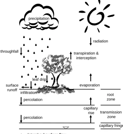
TOPLATS is a grid based and time continuous model. The vertical water fluxes of

5

the grid cells are calculated by the local SVATs (Fig. 1). The aggregation of local water fluxes yields in catchment scale vertical water fluxes. There is no lateral interaction between the local SVATs accounted for by the model. But based on the soils topo-graphic index of the TOPMODEL approach (Beven et al., 1995) a lateral redistribution of water is realized by adaptation of the local groundwater levels which are used as

10

lower boundary conditions of the local SVATs. Finally based flow is generated from the integration of local saturated subsurface fluxes along the channel network. A rout-ing routine is not integrated in the model. The basic hydrological processes and their representation in the TOPLATS model are summarized in Table 1.

In vertical direction the soil is divided in 2 layers (root zone and transmission zone).

15

An exponential decay function of saturated conductivity with depth is assumed. The soil water flow is calculated using an approximation for gravity driven drainage, and capillary rise is calculated based on the approach of Gardner (1958), both approaches using the Brooks and Corey parameterisation. Soil parameters are derived using the pedotransfer-function of Rawls and Brakensiek (1985). Plant growth is described by

20

plant specific plant development functions. There the seasonal change of plant param-eters is realised by updating plant parameter sets consisting of e.g. leaf area index, plant height and stomatal resistance. Plant growth itself is not simulated. The digital elevation model serves as basic data set for the calculation of the topographic wetness index (Beven et al., 1995), which is extended to a soils-topographic index (see Table 1)

25

accounting for local differences in transmissivity. For further details about the model the reader is referred to Famiglietti and Wood (1994a) and Peters-Lidard et al. (1995). The TOPLATS model has been successfully applied in several studies at different scales and in different climate regions around the world. Famiglietti and Wood (1994b)

(8)

HESSD

2, 2183–2217, 2005

Full Screen / Esc

EGU applied TOPLATS to the tallgrass prairie in the United States. Appropriate scales range

from sites to small catchments (∼12 km2) and from simulation of diurnal variations to water fluxes of a couple of weeks to be able to compare simulations to evapotranspi-ration measurements. Pauwels et al. (1999a, 1999b) extended the TOPLATS model to the application in high latitudes in Canada. They also focused on small scale

simula-5

tions but simulated water and energy fluxes for whole seasons.

Recent TOPLATS related publications more and more focus on regional applications and on the integration of remotely sensed data to improve the simulations. Endreny et al. (2000) examined the effects of the errors induced by the use of digital eleva-tion models derived from SPOT data and compared the simulaeleva-tion results to those

10

based on standard data sets (USGS 7.5-minute data set). Seuffert et al. (2002) cou-pled TOPLATS to an atmospheric model (Lokal-Modell of the German Meteorological Service) and applied the model to the regional scale Sieg catchment (about 2000 km2) in Western Germany. Pauwels et al. (2002) investigated the possibility to improve TOPLATS based simulation by the use of ERS derived soil moisture values at local

15

scale. A similar study was performed by Crow and Wood (2002) in the Red Arkansas basin who explored the benefit of coarse-scale soil moisture images for macro-scale model applications of TOPLATS (575 000 km2). And Crow et al. (2005) also exam-ined the possibility to upscale field-scale soil moisture measurements by means of distributed land surface modelling. In the context of this study they also expanded the

20

soil module within TOPLATS considering vertical soil heterogeneity. Finally Bormann and Diekkr ¨uger (2003) and Bormann et al. (2005) applied TOPLATS to the subhumid tropics of West Africa to simulate seasonal dynamics stream flow and soil moisture and found that poor data resolution and quality strongly limit the applicability of comparable models independent on scale.

25

Recapitulating TOPLATS has successfully been applied to a wide range of temporal and spatial scales in many different climate regions of the globe. The applicability seems to be limited by data availability and strongly depends on the aim of the study.

(9)

HESSD

2, 2183–2217, 2005

Full Screen / Esc

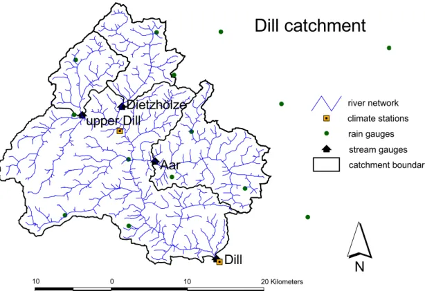
EGU 2.2. Catchment characteristics and available data sets of the Dill basin

The Dill catchment (693 km2) is located in central Germany and belongs to the Lahn-Dill low mountainous region. It is the target catchment of the SFB 299 (“Land use options for peripheral regions”) of the University of Gießen (Germany). Gauging stations exist for three sub-catchments (Upper Dill (63 km2), Dietzh ¨olze (81 km2) and Aar (134 km2))

5

as well as for the entire Dill catchment at Asslar (693 km2, Fig. 2).

The typical small scale topography ranges between 155 m and 694 m above sea level. The mean steepness of the slopes is approximately 14%. Mean annual rainfall ranges between 700 mm to 1100 mm depending on the location within the catchment and the corresponding elevation. Low precipitation areas show summer-dominated

10

precipitation and high precipitation areas winter-dominated precipitation regimes. Av-erage annual mean temperature is about 8◦C.

Soil parent material of the Lahn-Dill mountains is mainly argillaceous schist, greywacke, diabase, sandstone, quartzite, and basalt which developed during the De-von and Lower Carbon. During the Pleistocene periglacial processes have striongly

15

influenced the soil parent material. Therefore periglacial layers strongly influenced by the underlying geologic substrate are the main soil parent material of the catchment. Due to the heterogeneous nature of these periglacial layers, the pattern of soil types is complex. Main soil types are shallow cambisols, planosols derived from luvisols under hydromorphic conditions, and gleysols in groundwater influenced valleys.

20

Typical for most of the catchment area is a hard rock aquifer. Pore aquifers only exist in quaternary deposits such as river terraces or hillslope debris. Based on empir-ical relations the portion of baseflow contribution to discharge can be estimated to an amount of 9–16%. Most of the discharge of the Dill river is delivered through interflow. The contribution of surface runoff is estimated to be less than 10%.

25

Current land cover of the Dill area is dominated by forest. 29.5% of the catchment is covered by deciduous forest, 24.9% by coniferous forest. 20.5% of the catchment area is used for grassland and 6.5% agricultural crops. A portion of about 9% of the area

(10)

HESSD

2, 2183–2217, 2005

Full Screen / Esc

EGU is fallow land, and another 9% is covered by urban area. Obviously the Dill catchment

is a peripheral region dominated by extensive agriculture and forestry. Thanks to the SFB 299 of the University of Gießen a detailed data base is available for the whole Dill basin in 25 m resolution. Spatial data sets and time series (rain gauges, climate stations and stream gauges, for location of the stations see Fig. 2) used in this study

5

are summarised in Table 2. 2.3. Data aggregation

As the impact of increasing information loss on the calculation of regional scale wa-ter fluxes was to be investigated by this study, the available data set was aggregated stepwise to create grid based data sets of increasing grid size. Therefore the spatial

10

data sets (soil map, DEM, land use classification, land use scenarios) were system-atically aggregated applying standard aggregation methods provided by standard GIS software.

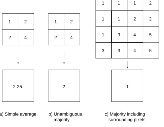
The aggregation of the DEM was carried out by calculating the simple averages of the pixels to be aggregated. Concerning soils and land use the data sets were

15

aggregated with respect to the majority of the pixels to be aggregated. The most fre-quent value was allocated to the aggregated pixel. If there is no unambiguous majority the surrounding pixels are included into the allocation (Fig. 3). Applying these algo-rithms, the DEM is smoothened by averaging, and mostly small homogenous areas of classified data (soils, land use) are shrinking or disappearing at the expense of large

20

homogenous areas.

3. Model application to the Dill catchment

3.1. Calibration and validation

In order to reduce the calibration of the TOPLATS model for application to the Dill basin to a minimum, parameterisation of the TOPLATS model was carried out by deriving

(11)

HESSD

2, 2183–2217, 2005

Full Screen / Esc

EGU or using directly as many parameters as possible from standard data bases. Thus

transferability of the model and the obtained results to other catchments is improved. Soil parameters were derived using the pedotransfer function of Rawls and Brakensiek (1985). Based on soil texture and porosity the parameters of the Brooks and Corey pa-rameterisation of soil retention characteristics are calculated (Brooks and Corey, 1964).

5

Topographic parameters were calculated directly from the digital elevation model, and plant parameters were taken from the PlaPaDa data base (Breuer et al., 2003). So the calibration could be reduced to an adjustment of plant specific stomatal resistances by a constant factor to meet the long-term water balance and to the calibration of the parameters of the base flow recession curve.

10

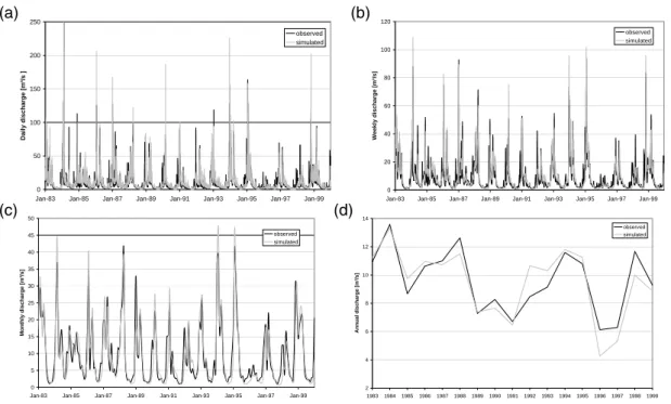
Figure 4 shows the simulation results for the entire Dill catchment (693 km2) com-pared to the observed values of the stream gauges. Calibration period is from 1983– 1989, validation period from 1990–1999. The accuracy of the simulation is satisfactory (quality measures see Table 3) considering that TOPLATS was calibrated only with re-spect to stomatal resistance and the baseflow recession curve. Quality measures for

15

the validation period are only slightly worse than for the calibration period. While for daily discharges the model efficiency (Nash and Suttliffe, 1970) is of moderate quality (0.65 for calibration, 0.61 for validation), the model efficiencies and coefficients of de-termination increase for longer time intervals (longer than one week) to values greater than 0.8. The mean bias in discharge between observations and simulations is about

20

5% for calibration and 12% for validation period.

For the simulation of the three subcatchments a recalibration was not carried out except the maximum baseflow parameter (baseflow at basin saturation). The simula-tion results for the Dietzh ¨olze (81 km2) and on the upper Dill (63 km2) are quite good while the results for the Aar catchment (134 km2) are of a moderate quality. Model

25

efficiencies for daily discharges range between 0.59 and 0.73 (calibration period) and between 0.52 and 0.69 (validation period). They increase with increasing time interval to values of 0.76 to 0.85 (weeks) and 0.82 to 0.90 (months). Quality measures and water balances for the Dill basin as well as for the three subcatchments are show in

(12)

HESSD

2, 2183–2217, 2005

Full Screen / Esc

EGU detail in Table 3.

Based on these simulations results it can be stated that TOPLATS can be applied to successfully simulate water balances on the regional scale in the low mountain range in temperate climates considering the minimum calibration strategy. Single peak flow events cannot be simulated with a high precision, but long-term water balances can be

5

simulated well just as well as seasonal variations of the water fluxes, and dry and wet periods within a season can be covered as well.

3.2. Model results based on increasing grid sizes

For all different grid sizes derived from the original data sets (10 grids ranging from 25 m to 2000 m resolution) continuous water balance simulations of 20 years were

10

performed. Based on this analysis the model specific minimum data resolution and therefore the minimum simulation effort required for good simulation quality aiming on water balance investigations can be determined.

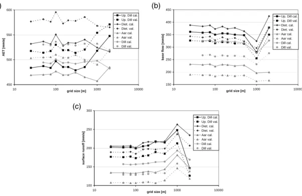
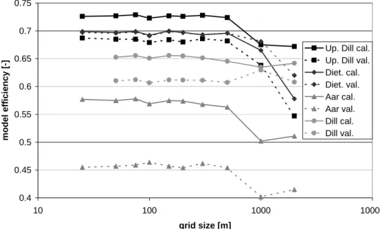
The computations reveal almost constant simulated annual water balances (Fig. 5) and model efficiencies (Fig. 6) for most of the grid sizes. Up to a grid size of 300 m

15

the simulated water fluxes remain almost constant except slight differences at indi-vidual grid sizes (e.g. at 100 m, which can be explained by differences in land use composition at the 100 m aggregation level) for individual water flows (e.g. for actual evapotranspiration). At a grid size of 500 m the differences slightly increase, and from 1000 m grid size onwards the simulation results get significantly worse, differences

in-20

crease. Thereby the results of the calibration period and the validation period again show the same regularity: if the simulation results are good for the calibration period, then also for the validation period good results are obtained. The same observation was made for bad agreement between the model and the measurements. This obser-vation is valid for all investigated catchments. Therefore no further separate analysis

25

for calibration and validation periods is required.

This statement concerning grid size dependent simulated water balances is also valid for the model efficiencies calculated from observations and model simulations.

(13)

HESSD

2, 2183–2217, 2005

Full Screen / Esc

EGU The model efficiencies – as expected from the simulated water balances – remain

con-stant up to a threshold value of 300 m to 500 m grid size. Model efficiencies for the 1000 m and the 2000 m grids are significantly lower. At this scale a significant and sys-tematic decrease of the quality measure is observed (Fig. 6). In addition to the results of the Dill catchment (Figs. 5 and 6), the Tables 4 and 5 summarise the scale

de-5

pendent model efficiencies and biases of stream flow calculated for all subcatchments within the Dill basin.

To investigate the influence of different land use distributions on the diverging be-haviour of simulated water balances for increasing grid sizes above a threshold of between 300 m and 500 m, three land use scenarios were used for further simulations.

10

For this study not the effect of the scenarios compared to the base line is of interest but again the effect of increasing grid size on the simulated scenario water balances. The scenarios were calculated by the “Proland model” (Fohrer et al., 2002) optimising the financial profit of the catchment area based on different field sizes (0.5, 1.5 and 5.0 hectares). So the spatial structures of the different land use scenarios differ a lot. If the

15

regularity of the results with respect to increase in grid size is the same for all scenarios and the baseline, then the land use distribution does not have major influence on the structure of the simulation results, and results on data aggregation are the transferable to other basins.

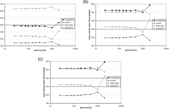
Figure 7 shows as an example the simulation results of the three different, field size

20

dependent scenarios for the Dill basin. It is obvious that simulated mean annual water flows only show minor differences up to a grid size of 500 m and significant differences for larger grid sizes. These exemplary results on different land use data sets for the upper Dill catchment are very similar to the results of the other three catchments. The other data sets show the same systematic reaction on data aggregation. Thus it can

25

be concluded that there is no significant impact of the spatial structure of land use on the regularity of the simulation results based on grid size aggregation.

(14)

HESSD

2, 2183–2217, 2005

Full Screen / Esc

EGU 4. Correlation between changes and catchment properties

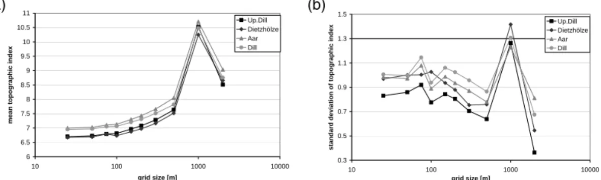
In order to analyse the influences of the different aggregated data sets on the grid size dependent simulation results an extended correlation analysis was carried out based on the statistics of catchment properties and water balance simulations. All spatial input data sets change significantly in statistics during aggregation. Increasing

5

the grid size leads to a smoothed surface of elevation and therefore to an increased mean topographic index (as cell size increases and slope in average decreases) and a decreasing standard deviation of the topographic index (Fig. 8). For single aggregation levels extreme values occur (e.g. 1000 m level for topographic index) while the tendency is the same for all investigated catchments.

10

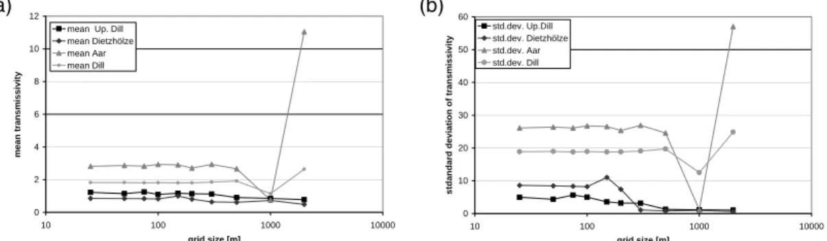
The transmissivity of the soils in general is barely affected by aggregation in a sys-tematic way. Single extreme values occur (Fig. 9) which does not show a homogenous tendency for the different catchments. The behaviour strongly depends on local soil hydraulic conditions and soil depths.

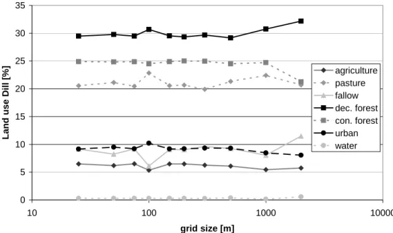
The effect of aggregation on the land use statistics is exemplarily shown for the entire

15

Dill basin by Fig. 10. It becomes clear that the aggregation has no major effect up to a cell size of 500 m. Only on the 100 m level significant deviations occur for pasture and fallow land. For grid sizes lager than 500 m significant changes in land use fractions can be observed for almost all land use classes. This is due to the fact that large areas grow at the expense of small areas, and grid sizes become much larger than the average

20

size of homogenous areas is. The effect of aggregation on land use fractions in the Dill catchment is comparable to the effects in the subcatchments which are summarised in Fig. 11.

To examine the contribution of the different data sources to the grid size depen-dent effects, a correlation analysis between water balance components and catchment

25

properties was carried out. The correlation coefficients for the entire Dill basin are summarised in Table 6.

(15)

HESSD

2, 2183–2217, 2005

Full Screen / Esc

EGU that land use has a major influence on the simulations. This can be approved by

the data. Forest areas are positively correlated to evapotranspiration and negative to stream flow production, while fallow areas and agricultural crops are correlated vice versa. Nevertheless one has to be careful because also spurious correlations appear in the data (contrary correlation coefficients of coniferous and deciduous forest), and

5

coherences between data and simulation results cannot be explained by linear corre-lations only. Nevertheless, water balance terms also show a clear dependence on soil and topographic characteristics. Surface runoff and base flow are highly correlated to the topographic index (surface runoff in a positive, base flow in a negative way), and transmissivity is correlated with base flow (positively) and evapotranspiration as well as

10

surface runoff (negatively).

So simulation results are related to all spatial data sets, and evaluation of the ef-fect of data aggregation therefore has to consider all data sources. Nevertheless it is worth to mention that predominantly the correlation between catchment properties (e.g. topographic index, transmissivity, land use) and simulated water flows varies from

15

catchment to catchment, in particular on the small scale.

5. Conclusions: Limitations of model application

This study indicates that an aggregation of input data for the calculation of regional water balances using TOPLATS type models does not lead to significant errors up to a grid size of 300 m. Between a grid size of 300 and 500 m a slight to partly significant

20

information loss leads to affected simulation results while applying a grid size of 1km and more causes significant errors in the computed water balance. If algorithms are integrated in a model taking into account subgrid variability further investigations are required.

The results of this study indicate that a meaningful aggregation of data should in the

25

first instance aim on preserving the areal fractions of land use classes, because land use is the most important information for this kind of SVAT schemes which are

(16)

domi-HESSD

2, 2183–2217, 2005

Full Screen / Esc

EGU nated by evapotranspiration. Nevertheless also the statistics of soil physical properties

and topography should not be neglected. Aiming on total stream flow often masks ef-fects of changes in fast and slow runoff components which may counterbalance their relative effects. Similar effects may also occur when effects of data aggregation and varying grid size point at different directions.

5

As the results for all different subcatchments and land use scenarios show similar structures, the findings are transferable to other catchments. The transferability to other model types is limited in so far, as TOPLATS focuses on vertical processes, and land use information is much more dominant than the influence of neighbouring grid cells. Therefore for models rather focusing on lateral processes which should be more

10

sensitive to a smoothing of the topography, the results need to be verified.

Concluding, this investigation shows that high quality simulation results require high quality input data but not always highly resolved data. The calculated water balances and statistical quality measures do not get significantly worse up to spatial data reso-lutions which should be available in almost all developed and also in many developing

15

countries. Therefore the focus should be set to improve data quality first and then to optimise data resolution secondly.

Acknowledgements. The authors thank the SFB 299 of the University of Gießen for

provid-ing the data set in the framework of the LUCHEM initiative (special thanks to the organisers L. Breuer and S. Huisman) and the authors of the TOPLATS model (E. Wood and W. Crow in

20

particular) for providing the model code and some support.

References

Beven, K.: Linking parameters across scales: subgrid parameterizations and scale dependent hydrological models, in: Scale issues in hydrological modelling, edited by: Kalma, J. D. and Sivapalan, M., Advances in hydrological processes, Wiley, 263–281, 1995.

25

Beven, K.J., Lamb, R., Quinn, P. F., Romanowicz, R., and Freer, J.: TOPMODEL, in: Computer Models of Watershed Hydrology, edited by: Singh, V. P., Water Resources Publications, 627–668, 1995.

(17)

HESSD

2, 2183–2217, 2005

Full Screen / Esc

EGU Bormann, H., Faß, T., Junge, B., Diekkr ¨uger, B., Reichert, B., and Skowronek, A: From local

hydrological process analysis to regional hydrological model application in Benin: concept, results and perspectives, Phys. Chem. Earth, 30, 347–356, 2005.

Bormann, H. and Diekkr ¨uger, B.: Possibilities and limitations of regional hydrological models applied within an environmental change study in Benin (West Africa), Phys. Chem. Earth,

5

28, 1323–1332, 2003.

Bormann, H., Diekkr ¨uger, B., and Renschler, C.: Regionalization concept for hydrological mod-elling on different scales using a physically based model: results and evaluation, Phys. Chem. Earth B, 24, 799–804, 1999.

Breuer, L., Eckhardt, K., and Frede, H.-G.: Plant parameter values for models in temperate

10

climates, Ecol. Model., 169, 237–293, 2003.

Brooks, R. H. and Corey, A .T.: Hydraulic properties of porous media, in: Hydrology Paper 3, 22–27, Colorado State University, Fort Collins, 1964.

Bruneau, P., Gascuel-Odoux, C., Robin, P., Merot, P., and Beven, K.: Sensitivity to space and time resolution of a hydrological model using digital elevation data, Hydrol. Process., 9, 69–

15

81, 1995.

Chen, E. and Mackay, D. S.: Effects of distribution-based parameter aggregation on spatially distributed agricultural nonpoint source pollution model, J. Hydrol. 295, 211–224, 2004. Crow, W. T. and Wood, E. F.: The value of coarse-scale soil moisture observations for surface

energy balance modeling, J. Hydrometeorol., 3, 467–482, 2002.

20

Crow, W. T., Ryu, D., and Famiglietti, J. S.: Upscaling of field-scale soil moisture measurements using distributed land surface modeling, Adv. Water Resour., 28, 1–5, 2005.

Endreny, T. A., Wood, E. F., and Lettenmaier, D. P.: Satellite-derived elevation model accuracy: hydrological modeling requirements, Hydrol. Process., 14, 177–194, 2000.

Famiglietti, J. S. and Wood, E. F.: Multiscale modelling of spatially variable water and energy

25

balance processes, Water Resour. Res., 30, 3061–3078, 1994a.

Famiglietti, J. S. and Wood, E. F.: Application of multiscale water and energy balance models on the tallgrass prairie, Water Resour. Res., 30, 3079–3093, 1994b.

Farajalla, N. and Vieux, B.: Capturing the essential variability in distributed hydrological model-ing: infiltration parameters, Hydrol. Process., 9, 55–68, 1995.

30

Fohrer, N., M ¨oller, D., and Steiner, N.: An interdisciplinary modelling approach to evaluate the effects of land use change, Phys. Chem. Earth, 27, 655–662, 2002.

(18)

HESSD

2, 2183–2217, 2005

Full Screen / Esc

EGU application to evaporation from a water table, Soil Sci., 85, 228–239, 1958.

HLBG: Hessische Verwaltung f ¨ur Bodenmanagement und Geoinformation, Digitales Gel ¨andemodell DGM25, date of access: 29 August 2005, in: http://www.hkvv.hessen.de/, 2000.

HLUG: Hessisches Landesamt f ¨ur Umwelt und Geologie, Digital soil map 1:50 000, 1998.

5

HLUG: Hessisches Landesamt f ¨ur Umwelt und Geologie. Stream gauges in the Lahn basin, date of access: 29 August 2005, http://www.hlug.de/medien/wasser/pegel/pg lahn.htm, 2005.

Kuo, W.-L., Steenhuis, T. S., McCulloch, C. E., Mohler, C. L., Weinstein, D. A., DeGloria, S. D., and Swaney, D. P.: Effect of grid size on runoff and soil moisture for a variable-source-area

10

hydrology model, Water Resour. Res., 35, 3419–3428, 1999.

Lahmer, W., Pf ¨utzner, B., and Becker, A.: Data-related Uncertainties in Meso- and Macroscale Hydrological Modelling, in: Accuracy 2000. Proceedings of the 4th international symposium on spatial accuracy assessment in natural resources and environmental sciences, edited by: Heuvelink, G. B. M. and Lemmens, M. J. P. M., Amsterdam, 389–396, 2000.

15

Milly, P. C. D.: An event based simulation model of moisture and energy fluxes at a bare soil surface, Water Resour. Res., 22, 1680–1692, 1986.

Monteith, J. L.: Evaporation and environment, in: Sympos. The state and movement of water in living organism, edited by: Fogy, G. T., Cambridge Univ. Press, 205–234, 1965.

Moore, I. D., Lewis, A., and Gallant, J. C.: Terrain attributes: Estimation methods and scale

20

effects, in: Modelling change in environmental systems, edited by: Jakeman, A. J., Beck, M. B., and McAleer, M., Wiley, New York, 189–214, 1993.

Nash, J. E. and Sutcliffe, J. V.: River flow forecasting through conceptual models, part I – a discussion of principles, J. Hydrol., 10, 272–290, 1970.

Omer, R. C., Nelson, E. J., and Zundel, A. K.: Impact of varied data resolution on hydraulic

25

modelling and floodplain delineation, J. Am. Water Resour. As., 39, 467–475, 2003.

Pauwels, V. R. N., Hoeben, R., Verhoest, N. E. C., De Troch, F. P., and Troch, P. A.: Improve-ment of TOPLATS-based discharge predictions through assimilation of ERS-based remotely sensed soil moisture values, Hydrol. Process., 16, 995–1013, 2002.

Pauwels, V. R. N. and Wood, E. F.: A soil-vegetation-atmosphere transfer scheme for the

mod-30

eling of water and energy balance processes in high latitudes. 1. Model improvements, J. Geophys. Res., 104, 27 811–27 822, 1999a.

(19)

mod-HESSD

2, 2183–2217, 2005

Full Screen / Esc

EGU elling of water and energy balance processes in high latitudes, 2. Application and validation,

J. Geophys. Res., 104, 27 823–27 840, 1999b.

Peters-Lidard, C. D., Zion, M. S., and Wood, E. F.: A soil-vegetation-atmosphere transfer scheme for modeling spatially variable water and energy balance processes, J. Geophys. Res., 102, 4303–4324, 1997.

5

Quinn, P., Beven, K., Chevallier, P., and Planchon, O.: The prediction of hillslope flow paths for distributed hydrological modelling using digital terrain models, Hydrol. Proces., 5, 59–79, 1991.

Rawls, W. J. and Brakensiek, D. L.: Prediction of soil water properties for hydrological modeling; in: Proceedings of the symposium watershed management in the eighties, edited by: Jones,

10

E. and Ward, T. J., Denver, 293–299, 1985.

Seuffert, G., Gross, P., and Simmer, C.: The Influence of Hydrologic Modeling on the Predicted Local Weather: Two-Way Coupling of a Mesoscale Weather Prediction Model and a Land Surface Hydrologic Model, J. Hydrometeorol., 3, 505–523, 2002.

Sivapalan, M.: Prediction of ungauged basins: A grand challenge for theoretical hydrology,

15

Invited Commentary, Hydrol. Process., 17, 3163–3170, 2003.

Sivapalan, M., Beven, K., and Wood, E. F.: On hydrologic similarity, 2. A scaled model of storm turnoff production, Water Resour. Res., 23, 2266–2278, 1985.

Thieken, A., L ¨ucke, A., Diekkr ¨uger, B., and Richter, O.: Scaling input data by GIS for hydrologi-cal modelling, Hydrol. Process., 13, 611–630, 1999.

20

Wolock, D. M. and Price, C. V.: Effects of digital elevation model map scale and data resolution on a topography based watershed model, Water Resour. Res., 30, 3041–3052, 1994. Zhang, W. and Montgomery, D. R.: Digital elevation model grid size, landscape representation,

and hydrologic simulations, Water Resour. Res., 30, 1019–1028, 1994.

(20)

HESSD

2, 2183–2217, 2005

Full Screen / Esc

EGU

Table 1. Main processes and equations of the TOPLATS model.

Model part Process Approach

Local SVATs Interception Storage approach: storage capacity

is proportional to leaf area index

Potential evapotranspiration (PET) Penman Monteith equation

(plant specific PET) (Monteith, 1965)

Actual evapotranspiration Reduction of PET by actual soil moisture status

(al-ternative: solving energy balance equation)

Infiltration Infiltration capacity after Milly (1986)

(depending on soil properties and soil water status)

Infiltration excess runoff Difference between

rainfall rate and infiltration capacity

Saturation excess runoff Contributing areas derived from TOPMODEL;

ap-proach based on the soils topographic index

Percolation Gravity driven drainage

Capillary rise Capillary rise from local water table

based on Gardner (1958) using Brooks and Corey parameters

Lower boundary condition Top of capillary fringe

(= depth of local water table)

TOPMODEL Spatial distribution of water table depths Soils-topographic index

(Sivapalan, 1987)

base flow Exponential decay function; maximum

(21)

HESSD

2, 2183–2217, 2005

Full Screen / Esc

EGU

Table 2. Spatial data sets and time series available for the Dill catchment.

Domain Data source/gauge stations Resolution/classification Origin of data set

Space Digital soil map 25 m resolution, 149 classes

(soil types)

Digital soil map 1:50 000 HLUG (1998)

Land use classification 25 m resolution, 7 classes (deciduous

forest, coniferous forest, grassland, agri-cultural crops, fallow land, open water bodies and urban areas)

Derived from multi-temporal Land-sat images (from 1994 and 1995)

Digital elevation model 25 m resolution HLBG (2000)

3 land use scenarios 25 m resolution; 6 classes (mixed forest,

grassland, agricultural crops, fallow land, open water bodies and urban areas)

Land use distribution derived from Proland model (Fohrer et al., 2002)

Time 2 weather stations Daily resolution; 1980–1999;

tempeture, air humidity, wind speed, solar ra-diation

German Meteorological Service (DWD)

15 rain gauges Daily resolution; 1980–1999 German Meteorological Service

(DWD)

(22)

HESSD

2, 2183–2217, 2005

Full Screen / Esc

EGU

Table 3. Water balances and model efficiencies for the calibration (cal.) and validation periods

(val.) of the four stream gauges within the Dill basin.

Quality measure Cal./ Val.

Time interval Dill Upper Dill Dietzh ¨olze Aar Mean bias in annual

discharge Cal. Val. Annual Annual 4.7% 12.0% 8.9% 17.8% 6.6% 7.2% 11.4% 17.6% Model efficiency Cal.

Val. Daily Weekly Monthly Annual Daily Weekly Monthly Annual 0.65 0.81 0.84 0.90 0.61 0.79 0.82 0.80 0.73 0.85 0.90 0.80 0.69 0.84 0.88 0.64 0.69 0.82 0.87 0.86 0.69 0.83 0.87 0.92 0.59 0.76 0.82 0.78 0.52 0.77 0.82 0.63 Coefficient of determination Cal. Val. Daily Weekly Monthly Annual Daily Weekly Monthly Annual 0.71 0.81 0.86 0.91 0.68 0.81 0.85 0.78 0.74 0.85 0.90 0.89 0.74 0.86 0.91 0.78 0.74 0.83 0.88 0.87 0.73 0.83 0.88 0.91 0.63 0.77 0.83 0.94 0.62 0.78 0.83 0.66

(23)

HESSD

2, 2183–2217, 2005

Full Screen / Esc

EGU

Table 4. Grid size dependent model efficiencies (me) for the four (sub-)catchments of the Dill

basin (cal.= calibration period, val. = validation period).

Grid size Dill Upper Dill Dietzh ¨olze Aar me (cal) me (val) me (cal) me (val) me (cal) me (val) me (cal) me (val) 25 m – – 0.73 0.69 0.70 0.70 0.58 0.46 50 m 0.65 0.61 0.73 0.69 0.70 0.70 0.58 0.46 75 m 0.66 0.61 0.73 0.69 0.70 0.70 0.58 0.46 100 m 0.65 0.61 0.72 0.68 0.69 0.69 0.57 0.46 150 m 0.66 0.61 0.73 0.68 0.70 0.70 0.58 0.46 200 m 0.66 0.61 0.73 0.68 0.70 0.70 0.57 0.46 300 m 0.65 0.61 0.73 0.69 0.69 0.69 0.57 0.46 500 m 0.65 0.61 0.72 0.68 0.70 0.70 0.56 0.45 1000 m 0.64 0.63 0.68 0.64 0.67 0.68 0.50 0.40 2000 m 0.64 0.61 0.67 0.55 0.58 0.62 0.51 0.42

(24)

HESSD

2, 2183–2217, 2005

Full Screen / Esc

EGU

Table 5. Grid size dependent biases of total stream flow for the entire simulation period (bias

(Qt), (%)) for the four (sub-)catchments of the Dill basin.

Grid size Dill Bias (Qt) (%) Upper Dill Bias (Qt) (%) Dietzh ¨olze Bias (Qt) (%) Aar Bias (Qt) (%) Cal. Val. Cal. Val. Cal. Val. Cal. Val. 25 m – – 2.7 15.2 0.6 2.7 2.0 0.3 50 m 0.6 –0.4 1.8 14.4 –0.2 1.7 1.5 –0.3 75 m 1.0 –0.1 2.3 15.0 0.7 2.6 1.7 –0.5 100 m 0.6 –1.8 –0.1 12.1 –2.6 –1.2 0.0 -2.1 150 m 0.8 –0.3 1.9 14.4 1.2 3.3 2.0 –0.1 200 m 0.6 –0.6 2.1 14.5 0.1 2.1 1.8 –0.1 300 m 1.0 0.2 3.3 15.4 0.5 2.7 0.4 –2.0 500 m 0.2 –0.5 2.4 41.3 –1.3 0.7 2.8 2.8 1000 m –2.0 –2.0 –3.4 7.3 –3.4 3.0 2.6 2.6 2000 m 3.3 3.8 –4.5 9.1 11.7 13.0 –1.8 –1.6

(25)

HESSD

2, 2183–2217, 2005

Full Screen / Esc

EGU

Table 6. Correlation coefficients (Pearson) between input data (transmissivity, topographic

index, land use) and model results (water balances, biases) for the entire Dill catchment.

Catchment property Bias in stream flow Stream flow Surface runoff Base flow Actual ET Crops 0.18 0.25 –0.54 0.53 –0.19 Pasture –0.57 –0.63 0.39 –0.60 0.62 Fallow 0.80 0.85 0.05 0.37 –0.92 Deciduous forest 0.47 0.42 0.43 –0.12 –0.51 Coniferous forest –0.81 –0.78 –0.17 –0.25 0.79 Urban –0.46 –0.51 –0.63 0.24 0.74 Open water 0.92 0.89 –0.31 0.66 –0.76 Forest –0.78 –0.81 0.34 –0.64 0.70 Agriculture –0.73 –0.78 0.21 –0.53 0.79 Mean topographic index –0.14 –0.12 0.98 –0.80 –0.15 Standard deviation of

topographic index –0.79 –0.75 0.40 –0.67 0.56 Mean transmissivity 0.95 0.92 –0.46 0.79 –0.77 Standard deviation of

(26)

HESSD

2, 2183–2217, 2005

Full Screen / Esc

EGU lateral subsurface flow

capillary fringe transmission zone root zone percolation surface runoff infiltration evaporation percolation capillary rise radiation transpiration & interception precipitation throughfall leaf drip

Fig. 1. Hydrological processes of the local SVATs represented by the TOPLATS model

(27)

HESSD

2, 2183–2217, 2005

Full Screen / Esc

Print Version Interactive Discussion EGU

;

# # # # # # # # # # # # # # # # % [ % [

_N

;

# % [

Dill catchment

river network climate stations rain gauges stream gauges catchment boundary 10 0 10 20 Kilometers

Aar

Dill

upper Dill

Dietzhölze

Fig. 2. Subcatchments (upper Dill, Dietzh ¨olze, Aar), rain and stream gauges in the Dill

(28)

HESSD

2, 2183–2217, 2005

Full Screen / Esc

EGU

a) Simple average b) Unambiguous majority c) Majority including surrounding pixels 1 2 4 2 1 2 4 2 1 2 4 3 2.25 2 1 1 1 3 3 4 5 5 2 2 1 1 1

Fig. 3. Algorithms for systematic aggregation of spatial data sets: simple average (a) for DEM

aggregation, majority(b) for aggregation of land use and soils, and consideration of the

(29)

HESSD

2, 2183–2217, 2005

Full Screen / Esc

Print Version Interactive Discussion EGU (a) 0 50 100 150 200 250

Jan-83 Jan-85 Jan-87 Jan-89 Jan-91 Jan-93 Jan-95 Jan-97 Jan-99

Dai ly d isch arg e [ m ³/ s ] observed simulated (b) 0 20 40 60 80 100 120

Weekly dischar ge [ m ³/ s] observed simulated (c) 0 5 10 15 20 25 30 35 40 45 50

Monthly discharge [m³/s] observed simulated (d) 2 4 6 8 10 12 14 19831984 19851986198719881989 199019911992199319941995 1996199719981999 A nnual dischar ge [m³/s] observed simulated

Fig. 4. Hydrographs of the Dill catchment: comparison of observed vs. simulated data in daily (a), weekly (b), monthly (c) and annual (d) resolution.

(30)

HESSD

2, 2183–2217, 2005

Full Screen / Esc

Print Version Interactive Discussion EGU (a) 450 500 550 600 10 100 _{grid size [m]} 1000 10000 A E T [ mm/ a ]

Up. Dill cal. Up. Dill val. Diet. cal. Diet. val. Aar cal. Aar val. Dill cal. Dill val. (b) 150 200 250 300 350 400 450 10 100 1000 10000 grid size [m] base flow [m m /a]

Up. Dill cal. Up. Dill val. Diet. cal. Diet. val. Aar cal. Aar val. Dill cal. Dill val. (c) 100 150 200 250 300 10 100 _{grid size [m]} 1000 10000 sur face r unoff [m m /a]

Up. Dill cal. Up. Dill val. Diet. cal. Diet. val. Aar cal. Aar val. Dill cal. Dill val.

Fig. 5. Grid size dependence of simulated annual water fluxes: actual evapotranspiration (AET) (a), base flow (b) and stream flow (c) of the Dill basin and its three subcatchments (Up. Dill

= Upper Dill, Diet. = Dietzh¨olze). Calibration periods and validation (cal., val.) periods are analysed separately.

(31)

HESSD

2, 2183–2217, 2005

Full Screen / Esc

Print Version Interactive Discussion EGU 0.4 0.45 0.5 0.55 0.6 0.65 0.7 0.75 10 100 1000 10000 grid size [m] m odel effi ci ency [-]

Up. Dill cal. Up. Dill val. Diet. cal. Diet. val. Aar cal. Aar val. Dill cal. Dill val.

Fig. 6. Dependence of model efficiencies (based on daily simulations) on grid sizes for the

Dill basin and its three subcatchments (Up. Dill= Upper Dill, Diet. = Dietzh¨olze). Calibration periods and validation (cal., val.) periods are analysed separately.

(32)

HESSD

2, 2183–2217, 2005

Full Screen / Esc

Print Version Interactive Discussion EGU (a) 100 200 300 400 500 600 700 10 100 1000 10000 grid size [m] me a n a nnua l wa te r f lows [ mm/ a ] streamflow runoff base flow actual ET (b) 100 200 300 400 500 600 10 100 1000 10000 grid size [m] me a n a nnua l wa te r f lows [ mm/ a ] streamflow runoff base flow actual ET (c) 100 200 300 400 500 600 10 100 1000 10000 grid size [m] me a n a nnua l wa te r f lows [ mm/ a ] streamflow runoff base flow actual ET

Fig. 7. Grid size dependent simulation results of the three different land use scenarios (0.5 ha

(33)

HESSD

2, 2183–2217, 2005

Full Screen / Esc

Print Version Interactive Discussion EGU (a) 6 6.5 7 7.5 8 8.5 9 9.5 10 10.5 11 10 100 1000 10000 grid size [m] m ean topogr aphi c i ndex Up.Dill Dietzhölze Aar Dill (b) 0.3 0.5 0.7 0.9 1.1 1.3 1.5 10 100 1000 10000 grid size [m] standar d devi ati on of topogr aphi c i ndex Up.Dill Dietzhölze Aar Dill

Fig. 8. Grid size dependent statistics of topographic catchment properties of the Dill catchment:

(34)

HESSD

2, 2183–2217, 2005

Full Screen / Esc

Print Version Interactive Discussion EGU (a) 0 2 4 6 8 10 12 10 100 1000 10000 grid size [m] m ean tr ansm issivity

mean Up. Dill mean Dietzhölze mean Aar mean Dill (b) 0 10 20 30 40 50 60 10 100 1000 10000 grid size [m] stdandar d deviation of tr ansm issivity std.dev. Up.Dill std.dev. Dietzhölze std.dev. Aar std.dev. Dill

Fig. 9. Grid size dependent statistics of soil hydrological catchment properties of the Dill

(35)

HESSD

2, 2183–2217, 2005

Full Screen / Esc

Print Version Interactive Discussion EGU 0 5 10 15 20 25 30 35 10 100 1000 10000 grid size [m] La nd us e D ill [ % ] agriculture pasture fallow dec. forest con. forest urban water

(36)

HESSD

2, 2183–2217, 2005

Full Screen / Esc

Print Version Interactive Discussion EGU (a) 0 5 10 15 20 25 30 35 40 45 50 10 100 1000 10000 grid size [m] La nd us e uppe r D ill [ % ] agriculture pasture fallow dec. forest con. forest urban water (b) 0 5 10 15 20 25 30 35 40 45 50 10 100 1000 10000 grid size [m] Land use D iet z hölz e [ % ] agriculture pasture fallow dec. forest con. forest urban water

Fig. 11. Grid size dependent statistics of land cover classes of the upper Dill (a) and the