HAL Id: hal-00110572
https://hal.archives-ouvertes.fr/hal-00110572
Submitted on 20 Nov 2018
HAL is a multi-disciplinary open access
archive for the deposit and dissemination of
sci-entific research documents, whether they are
pub-lished or not. The documents may come from
teaching and research institutions in France or
abroad, or from public or private research centers.
L’archive ouverte pluridisciplinaire HAL, est
destinée au dépôt et à la diffusion de documents
scientifiques de niveau recherche, publiés ou non,
émanant des établissements d’enseignement et de
recherche français ou étrangers, des laboratoires
publics ou privés.
Renaud Toussaint, Jørgen Akselvoll, Geir Helgesen, Arne T. Skjeltorp, Eirik
Grude Flekkøy
To cite this version:
Renaud Toussaint, Jørgen Akselvoll, Geir Helgesen, Arne T. Skjeltorp, Eirik Grude Flekkøy.
Interac-tion model for magnetic holes in a ferrofluid layer. Physical Review E : Statistical, Nonlinear, and Soft
Matter Physics, American Physical Society, 2004, 69 (1), pp.011407. �10.1103/physreve.69.011407�.
�hal-00110572�
Interaction model for magnetic holes in a ferrofluid layer
Renaud Toussaint*Department of Physics, NTNU, N-7491 Trondheim, Norway
Jo”rgen Akselvoll, Geir Helgesen, and Arne T. Skjeltorp Institutt for Energiteknikk, N-2007 Kjeller, Norway
Eirik G. Flekko”y
Department of Physics, University of Oslo, N-0316 Oslo, Norway 共Received 30 April 2003; published 30 January 2004兲
Nonmagnetic spheres confined in a ferrofluid layer共magnetic holes兲 present dipolar interactions when an external magnetic field is exerted. The interaction potential of a microsphere pair is derived analytically, with precise care for the boundary conditions along the glass plates confining the system. Considering external fields consisting of a constant normal component and a high frequency rotating in-plane component, this interaction potential is averaged over time to exhibit the average interparticular forces acting when the imposed frequency exceeds the inverse of the viscous relaxation time of the system. The existence of an equilibrium configuration without contact between the particles is demonstrated for a whole range of exciting fields, and the equilibrium separation distance depending on the structure of the external field is established. The stability of the system under out-of-plane buckling is also studied. The dynamics of such a particle pair is simulated and validated by experiments.
DOI: 10.1103/PhysRevE.69.011407 PACS number共s兲: 82.70.Dd, 75.50.Mm, 75.10.⫺b, 83.10.Pp
I. INTRODUCTION
The dynamic properties of so-called magnetic holes in ferrofluid layers has been the object of increasing interest over the past 20 years 关1–23兴. These systems consist of spherical nonmagnetic particles in a carrier ferrofluid, whose size is order of magnitudes共1–100m兲 above the one of the magnetic particles 共0.01 m兲 in suspension. The ferrofluid appears then as homogeneous at the scale of the large particles—holes— and their effect on the magnetic field can be modeled as a dipolar perturbation, where the magnetic moment is opposite to the one of the displaced ferrofluid关1兴. The system is generally confined between glass plates in quasi-two-dimensional layers, whose thickness slightly ex-ceeds the diameter of the holes. The induced dipolar interac-tions give rise to a rich zoology of physical phenomena, such as crystallization of magnetic holes in constant or oscillating magnetic fields 关1–5兴, order-disorder transitions in those crystals 关6–9兴, or nonlinear phenomena in the dynamics of those systems in low frequency oscillating fields 关10–13兴, commonly described using braid theory关14–18兴.
The understanding of these systems is important in rela-tion to industrial ferrofluid applicarela-tions 关24,25兴, or for their potential use in biomedicine关26–28兴. The dynamics of these phenomena can also be used indirectly to characterize the ferrofluid’s transport properties 关29兴, such as its viscosity. Eventually, the ability to shape the effective pair interaction potentials through the imposed external magnetic field makes these systems good candidates as large analog models to study phase transitions关30兴, aggregation phenomena 关19兴, or fracture phenomena in coupled granular/fluid systems.
Nonetheless, despite the theoretical studies on similar dual systems such as ferromagnetic particles in a viscous fluid关31,32兴, and the extensive experimental observations of these magnetic holes, there is a lack of theory describing this detailed effective pair interaction potential. Notably, there has been no satisfying explanation so far for the existence of stable configurations of particle populations with finite sepa-ration distances in external fields consisting of a circular ro-tating in-plane component and a constant normal one 共re-ported in Ref. 关2兴兲, or for the existence of out-of-plane buckled structures关8兴, and no theoretical framework for the influence of the ferrofluid layer thickness 共separation of the embedding plates兲.
We will show here how the magnetic boundary conditions along the confining plates lead to rich effective interaction potentials rendering for those structures, rather than the qualitative magnetohydrodynamic effects proposed in Ref.
关2兴. In particular, we give an explanation for the existence of
a finite equilibrium separation between particles. Theoretical work has already been done along this line 关20兴, but in a reduced case of constant normal field. The present study in-cludes a circular high frequency oscillating field in addition. The potential derived should be an essential brick in all the applications mentioned above of the magnetic holes, and in general this type of contribution of the confining structure should be relevant to any quasi-two-dimensional共2D兲 colloi-dal system with a significant dielectric or magnetic perme-ability contrast between the fluid medium and the confining structure, as in Ref.关33兴.
In this paper, we first describe the system under study and review briefly the basic modeling assumptions and standard theory. We next derive the instantaneous pair interaction po-tential with precise care for the magnetic permeability con-trast of the boundaries, and average it over the short oscilla-*Electronic address: [email protected]
tion periods to get the effective interactions. We turn then to the properties of the equilibrium configurations, sketch a simple dynamical theory, and compare the theoretical and experimental results for the dynamics of a particle pair. Eventually, the three-dimensional aspect of the ferrofluid lay-ers is taken into account to evaluate both gravity-induced corrections and the stability of the system under out-of-plane buckling.
II. SYSTEM UNDER STUDY AND BASIC ASSUMPTIONS
The system considered consists of two nonmagnetic spheres inside a ferrofluid which is homogeneous at their scale, whose susceptibility and magnetic permeability are denoted, respectively, f and f⫽0(1⫹f), where 0
⫽4⫻10⫺7H m⫺1. This ferrofluid is itself embedded be-tween two glass plates considered as perfectly plane, parallel, and nonmagnetic. The magnetic field anywhere between the glass plates is then decomposed between a uniform order zero component resulting from the outer imposed field, plus a perturbation due to the spheres. This perturbation is essen-tially dipolar: an isolated sphere in a field with a given uni-form 共constant兲 boundary value H at infinity provokes a purely dipolar perturbation outside it, generated by an effec-tive dipole as shown in Fig. 1:
⫽⫺V¯ H, 共1兲
¯⫽ f 1⫹2f/3
, 共2兲
where¯ is an effective susceptibility including a demagne-tization factor, i.e., whose precise form results when the boundary conditions for the magnetic field on the surface of the sphere are properly taken into account共see, for example, Refs.关20,34兴兲, SI magnetic units are adopted throughout this paper, V⫽a3/6 and a refer, respectively, to the volume and diameter of a sphere. This result justifies the name of mag-netic holes used for those nonmagmag-netic spheres, and stays valid to leading order when a system more complicated than an isolated sphere is considered: it holds as soon as the ex-ternal magnetic field H can be considered as uniform at the scale of a sphere, which will be assumed and commented on further in Sec. VI B.
The average magnetic field inside the ferrofluid H itself is simply related to the external uniform magnetic field im-posed outside the glass plates He through
H⫽H储e⫹ 1
1⫹f
H⬜e 共3兲
to fulfill the boundary conditions along the glass-ferrofluid planar interfaces—namely, H储e⫽H储 and B⬜e⫽B⬜ 关34,35兴— where the parallel and normal components are oriented rela-tive to the glass plates.
The simplest model for a particle pair can be obtained first by neglecting the effect of the nonmagnetic boundaries: con-sidering a couple of two such spheres of identical moments with a separation vector from center to center r, the total interaction energy of the system is, after Bleaney and Bleaney 关34兴, U⫽ f 4 2
冉
1⫺3 cos 2 r3冊
, 共4兲where r⫽储r储 and ⫽⬔共r;兲 is the angle between the field and the separation vector.
We consider now external fields composed of a circular in-plane component oscillating at frequency, superimposed to a constant normal one. At high enough frequency, the relative displacement of the particles during an oscillation period is negligible compared to its average value, and the time dependence of the separation vector can be decoupled in a slow and a fast varying mode, r(t)⫽r¯(t)⫹␦r(r¯;t), with
␦r⫽0 and ␦rⰆr¯ . Throughout the remainder of this paper, bold symbols refer to vectors, lightface ones to their norm, and the upper bar refers to averaged quantities over oscillat-ing time. Moreover, we will now use the additional con-straint on r that it should be in-plane under the effect of the glass plates over the microspheres which center them at po-sitions equally separated from the top and bottom bound-aries. The presence of the boundaries can indeed be repre-sented by equivalent image dipoles outside the confining plates, as established in Sec. III, which repel the dipole from the boundaries. This constraint will be addressed specifically in Sec. VII to show that this centering magnetic effect is valid in most work cases when no lateral confinement is exerted in the system—Sec. VII B. The possible sink caused by gravity under the density contrast between the micro-spheres and the fluid is generally negligible—Sec. VII A. Thus, in the reference frame (r¯ˆ;nˆ丢¯ˆ;nˆ)—where hats refer tor
unit vectors—instantaneous fields read
H⫽H共cossin␣;sinsin␣;cos␣兲T, 共5兲 with definition
cot␣⫽⫽H⬜/H储⫽H⬜e/共1⫹f兲H储e, 共6兲 and ⫽2t. Thus, defining ␥⫽⬔(r¯;r) comes cos2
⫽cos2(⫺␥)sin2␣⫽cos2(⫺␥)/(1⫹2), and
U共r;兲⫽Aa 3 r3关2 2⫺1⫺3 cos共2⫺2␥兲兴, 共7兲 with A⫽ f 2 8a3共1⫹2兲⫽ fa32H储2 288 . 共8兲
FIG. 1. Pair of nonmagnetic particles in a ferrofluid layer and related effective dipolar moments due to the external magnetic field.
Consider distant enough particles to prevent contact and sig-nificant hydrodynamic interactions during an oscillation pe-riod of the external field: the neglect of inertial terms allows one to balance magnetic interaction forces and Stokes drag for both particles, which gives, to leading order in ␦r/r¯,
3a共r¯˙⫹␦r˙兲⫽⫺“U共r兲 ⫽3Aa 3 r ¯4 关共2 2⫺1兲r¯ˆ⫹3 cos共2兲r¯ˆ ⫹2 sin共2兲nˆ丢¯ˆr兴. 共9兲
Neglecting inertial terms is easily justified since a large up-per bound of Reynold’s number can be evaluated as being Re⫽xa2/⭐10⫺4, where x⫽␦r/a is the relative ampli-tude of the oscillations which will be shown straightfor-wardly to be typically below 10⫺2, for typical diameters a
⫽50m, ferrofluid’s viscosity ⫽9⫻10⫺3Pa s and den-sity⫽1000 kg m⫺3, and field oscillation frequency⫽100 Hz. Random thermal motion in the ferrofluid is essentially irrelevant at these size scales, as will be shown in Sec. VI B, justifying the use of deterministic dynamics instead of a Brownian one. The above equations共7兲 and 共9兲 establish that the slow motion r¯ is driven by an effective potential obtained
through time averaging over the oscillations of the field, i.e., simply using cos2⫽1/2 at fixed r⫽r¯,
3ar¯˙⫽⫺“U¯共r¯兲, 共10兲 with U¯共r¯兲⫽Aa 3 r ¯3共2 2⫺1兲 共11兲
while small and quick elliptic oscillations are performed:
␦r⫽⫺c a5 r ¯5关3 sin共4t兲r¯⫹2 cos共4t兲nˆ丢¯r兴, with c⫽ A 42a3⫽ 0共1⫹f兲¯2H储2 1152 .
The relative magnitude of the fast oscillations ␦r/r¯
⫽ca
5/¯r5 are indeed negligible as soonⰇ
c⯝0.1 Hz for typical ferrofluids, f⫽1.9, ¯⫽0.84, ⫽9⫻10⫺3 Pa s and fields H储⫽14 Oe.c, inverse of the viscous relaxation time of the system, is the critical frequency introduced in Ref.
关11兴, above which a particle pair cannot anymore follow the
direction of an external rotating field due to the fluid drag. In this paper, we study regimes where⭓10 Hz, for which the relative variations of the separation vector are below 1%, and focus on the slow motion of the particles r¯(t) driven by
U¯ (r¯).
In this simple picture however, this average potential is a simple central one whose inverse cubic range reflects the dipole-dipole nature of the interactions, and in the absence of any characteristic length scale, this basic model predicts a very simple behavior for the particle pair. Depending on the
ratio  of the normal over the in-plane field, either the two particles will repel each other without end if ⬎c⫽1/
冑
2 or they will attract each other when⬍cuntil the magnetic forces are balanced by contact forces or very short-range hydrodynamic forces sensitive when particles almost touch—when (r⫺a)/a gets insignificant. This theory is ob-viously insufficient to render for the finite equilibrium sepa-ration distance, sometimes at a few diameters, which is ex-perimentally observed for a whole range of imposed fields关2兴. A proper treatment of the boundary conditions of the
system along the glass plates, introducing the plate separa-tion as an extra length scale to the problem, will in the fol-lowing section be shown to remedy this problem.
III. EFFECT OF THE BOUNDARIES ON THE INSTANTANEOUS INTERACTIONS
The boundaries between the ferrofluid and the embedding glass plates are supposed to be perfectly plane. The two mi-crospheres are supposed perfectly centered between the glass plates, and the perturbation of the magnetic field due to the presence of those spheres is modeled as a perturbation due to two identical pointlike dipoles⫽⫺¯ VH located at the cen-ter of the spheres. To fulfill the magnetic boundary conditions—i.e. the continuity of H储 and B⬜—along the plates, a direct use of the image method 共e.g., Weber 关36兴兲 shows that this magnetic perturbation between the plates is equal to the field emitted, in an unbounded uniform medium of susceptibilityf, by an infinite series of dipoles: the two original ones, at locations defined as 0 and x, plus an infinite set of images for each of them corresponding to the mirror symmetry across the plane boundaries of the sources and all of the successive images. A magnification factor
⫽f⫺0
f⫹0⫽
f
f⫹2 共12兲
multiplies the amplitude of the dipolar moments at each sym-metry operation, i.e., explicitly defined by the following con-ditions.
For any dipole sourceat position r0, with h the normal separation vector between the plates, an infinite set of dipolar images indexed by l苸Z is defined by their locations and moments—see Fig. 2:
rl⫺r0⫽lh, 共13兲
l储⫽兩l兩储, 共14兲
l⬜⫽兩l兩共⫺1兲兩l兩⬜. 共15兲 The total interaction energy of such a system—where all dipoles do not have anymore the same moment—is共Bleaney and Bleaney关34兴兲 U⫽ f 8 b
兺
⫽c 1 rbc3冋
b•c⫺ 3共b•rbc兲共c•rbc兲 rbc2册
, 共16兲where the sum on the b index runs over the two source di-poles and the one over the c index runs over the whole set of sources and image dipoles, as seen in the preceding section; separation vectors can be considered as constant over the quick variations of, and the upper bars over r are implicit for the remainder.
We will then use the following straightforward geometri-cal equalities resulting from Eqs.共1兲, 共6兲, 共13兲–共15兲: if the c index represents the lth image of the source b, then
b•c 兩l兩2 ⫽ 1⫹共⫺1兲l2 1⫹2 , 共17兲 共b•rbc兲共c•rbc兲 兩l兩2r bc 2 ⫽ 2共⫺1兲l 1⫹2 , 共18兲 rbc⫽兩l兩h. 共19兲
If on contrary c represents the lth image of one source—as indexed in Fig. 2—and b the other source, then
b•c 兩l兩2 ⫽ 1⫹共⫺1兲l2 1⫹2 , 共20兲 共b•rbc兲共c•rbc兲 兩l兩2r bc 2 ⫽
关y cos⫹共⫺1兲ll兴共y cos⫹l兲
共1⫹2兲共y2⫹l2兲 , 共21兲 rbc⫽
冑
x2⫹l2h2, 共22兲 where y⫽x h 共23兲is the ratio of the particle in-plane separation distance to the plate separation. Introducing these equalities in Eq. 共16兲 we get U 2Aa3⫽ I0so x3⫹l
兺
苸Z* 兩l兩冋
Il ss 兩l兩3h3⫹ Ilso 共x2⫹l2h2兲3/2册
, 共24兲 Ilss⫽1⫺2共⫺1兲兩l兩2, 共25兲 Ilso⫽冋
1⫹共⫺1兲兩l兩2 ⫺3关y cos⫹共⫺1兲 兩l兩l兴共y cos⫹l兲 共y2⫹l2兲册
, 共26兲where A is the constant defined in Eq. 共8兲. The first term, denoted by I0so, is the direct interaction between the two sources, the next one Il
ss
corresponds to the interactions be-tween the sources and their own images, and finally the term Ilso corresponds to the cross interactions between a source and the images of the other one.
IV. TIME-AVERAGED EFFECTIVE INTERACTIONS A. Derivation of the potential
The H fields consist of a perfectly circular in-plane com-ponent H储⫽H储关(cos)rˆ⫹(sin)nˆ丢rˆ兴, and a normal
com-ponent H⬜ which is maintained constant. During an oscilla-tion of the in-plane field, the only significantly varying quantity in Eq. 共16兲 is the angle, with once again cos2
⫽1/2.
The term Il ss
, i.e., the interactions between a source and its own images, naturally does not depend on the in-plane separation vector x, and produces no net in-plane force. It is worthwhile to note that this would however not be the case for any nonplane interfaces, giving the possibility to quench any geometrical property of the roughness of the interfaces in this potential. In the current hypothesis of purely planar plates, this interaction term is only responsible for a normal centering force, as will be established in Sec. VII B. For the present purpose where the microspheres are constrained on the half-plane between the plates, the in-plane forces are the only relevant ones, and this term is simply discarded in the following.
The remaining terms produce through time average the interaction energy U¯共x兲⫽Ad 3 h3u
冉
x h冊
, 共27兲with A the constant defined in Eq. 共8兲, and a dimensionless term u共y兲⫽共22⫺1兲y⫺3 ⫹4
兺
l⫽1 ⫹⬁ l冉
1⫹共⫺1兲 l2 共y2⫹l2兲3/2 ⫺ 3 2 y2⫹2共⫺1兲ll22 共y2⫹l2兲5/2冊
. 共28兲The first term reduces to the expression of the first-order theory of Eq.共11兲, which is a test of self-consistency, since an infinite medium would be equivalent to the absence of permeability contrast along the plates, ⫽0. The following ones render for the interactions between a source and the images of the other one. Due to the cylindrical symmetry of the problem with a purely circular in-plane field, this inter-action is isotropic: the dependence on the separation vector x enters only through its norm x⫽hy.
B. Properties of the isotropic interactions
The introduction of those images is responsible for pos-sible finite separation equilibrium distances for a whole range of characterizing the imposed magnetic field, as is illustrated in Fig. 3: In this example, a typical susceptibility f⫽1.9 was considered for the ferrofluid, i.e.,⫽0.49. The four potentials u(y ) represented correspond, respectively, to ⫽0.4, 0.58, 0.8, 2.1. They were obtained by truncating the
sums in Eq. 共28兲 to order l⫽10, which corresponds to a relative error lower than 10⫺3 in u for any y.
The general typology of those potentials can be classified in four cases as will be demonstrated in the following sec-tion, separated by three particular values of, referred to as m, c, and u, which depend only on the susceptibility f.
共a兲 For⬍m, u is a monotonically increasing function, and the magnetic forces are purely attractive, thus leading any pair of spheres to contact.
共b兲 For m⬍⬍c, u presents a short-range attractive core, and presents both a maximum—an unstable equilib-rium point—at some distance yi, typically slightly below 1, and a minimum—a stable equibrium point—at a greater dis-tance ys, usually above 1.
Two locally stable equilibrium configurations are possible in principle, depending on the ratio ya⫽a/h of the particle diameter to the plate separation, and of the initial particle separation yinit: if yinit⬎yi, the particles should end up at the equilibrium separation ys, which since ys⬎1⬎ya corre-sponds to an equilibrium configuration without contact be-tween the particles. If on the contrary yinit⬍yi, the particles should attract each other and end up in contact at ya. Since any separation y⬍ya is forbidden due to contact forces, this second case is only possible when ya⬍yi, i.e., when the ratio of plate separation over particle diameter is sufficiently big. In that case, if the thermal fluctuations are large enough to let the particles go over the energy maximum at yi with a significant probability over the observation time, only one of the two possible equilibrium configurations will be thermo-dynamically stable, and the other one will be only meta-stable. The selection of stability/metastability between the two is determinated by the comparison of u(ya) and u(ys).
共c兲 For c⬍⬍u, u presents only a global minimum, which thus corresponds to a stable equilibrium separation distance ys. Since generally ys⬎1⬎ya, this equilibrium configuration corresponds to a finite separation distance hys⫺a⬎0.
共d兲 For u⬍, u is monotonically decreasing, and the time-averaged magnetic forces are purely repulsive at any separation.
V. EQUILIBRIUM SEPARATION DISTANCE AS FUNCTION OF THE APPLIED FIELD
The separation equilibrium distance yeq—which is stable or not—corresponds to the extrema of the potential, and can be obtained in principle by solving
du
d y共yeq兲⫽0. 共29兲 yeqcorresponds to ysor yidefined in Sec. IV B, according to the sign of d2u/d y2. Derivating Eq.共28兲 with respect to the scaled separation y leads straightforwardly to
y4 3 du dy⫽共1⫺2 2兲⫺2
兺
l⫽1 ⫹⬁ l l共y兲关⫺1⫹2共⫺1兲l2兴, 共30兲 l共y兲⫽ 共y2⫺4l2兲y5 共y2⫹l2兲7/2 . 共31兲Equation 共30兲 above is the sum of a term independent of plus another proportional to 2. The constant term can be shown to be positive, and the prefactor of2 strictly nega-tive, for any possible (y ,), i.e., any y⬎0, 0⭐⬍1. Thus, du/d y (y ,) is a monotonic decreasing function of2, equal to 0 when 0共y兲⫽
冪
1⫹2兺
l⫽1 ⫹⬁ l l共y兲 2⫹4兺
l⫽1 ⫹⬁ 共⫺1兲ll l共y兲 . 共32兲Thus, for a given field configuration , and separation y, pair interactions are attractive, i.e., du/d y⬎0, if 
⬍0(y ), and conversely if⬎0( y ). A numerical study of
the above function, for any, shows that0(y ) is
monotoni-cally decreasing fromc⫽1/
冑
2 to a finite positive minimum m() between y⫽0 to ym(), and next monotonically in-creasing up to a finite limit u()⬎c between ym() and y→⫹⬁.These considerations allow us to obtain by a direct graphical inversion of 0(y ) the possible roots ys() and yi() for which the interaction forces are zero at a given field geometry , as shown in Fig. 4 which is obtained for the particular casef⫽1.9, i.e.,⫽0.49. This nonlinear de-pendence of the equilibrium separation ys() seems more complex than observed in earlier experiments by Helgesen and Skjeltorp关2兴. This apparent discrepancy will be resolved in the following section, which is centered on finite-time results.
Defining the three parametersm,c,u identified above as c⫽0共y⫽0兲, 共33兲 m⫽min y 0共y兲⫽0共ym兲, 共34兲 u⫽ lim y→⫹⬁ 0共y兲, 共35兲
these arguments prove that the pair effective potentials be-long to one of the four types described in the preceding sec-tion.
共a兲 If ⬍m, the potential is purely attractive at any separation.
共b兲 If m⬍⬍c, there are two roots to Eq. 共29兲, de-noted yi() and ys(): the potential is attractive below yior above ys and repulsive between both.
共c兲 If c⬍⬍u, the potential presents a single mini-mum at ys().
共d兲 If⬎u, the potential is purely repulsive and there is no equilibrium separation.
The definition ofuabove—Eq.共35兲—shows also clearly that lim→
u
⫺(ys)⫽⫹⬁: in principle, it should be possible to drive a pair of microspheres in an equilibrium configuration with any desirable separation distance. Naturally, since the magnetic interactions decay rapidly with distance, thermal processes or any kind of external perturbation in the fluid flow, or default in the planarity of the plates, will be pre-dominant at large separations, where this theory will become inapplicable.
The dependence ofc,u,mon the susceptibility of the ferrofluid共through the parameter兲 is as follows: Replacing
l(0)⫽0 in Eq. 共32兲 shows that
c⫽1/
冑
2 共36兲independent of . Similarly, since limy→⫹⬁l(y )⫽1, u is easily summed as
FIG. 4. Equilibrium separation of a pair as a function of the applied field.
u⫽ 1
冑
2冪
1⫹2兺
l⫽1 ⫹⬁ l 1⫹2兺
l⫽1 ⫹⬁ 共⫺兲l ⫽ 1冑
2 1⫹ 1⫺. 共37兲A numerical study of m shows that it decreases monotoni-cally with, down to zero when→1.
This shows that the range ofover which stable equilib-rium distances exist is larger when the susceptibility of the ferrofluid is important共increases withf; mandu are, respectively, decreasing and increasing with 兲 up to the limiting case of an infinitely susceptible ferrofluid →1 (fⰇ1), for whichm→0, u→⫹⬁, and there is a finite stable equilibrium separation for any ratio.
The other limiting case →0 is obtained directly by dis-carding the sums in Eq.共32兲—their convergence to 0 in that limit for any y is straightforward. This shows that lim→0m⫽lim→0u⫽c⫽1/
冑
2. Without any permeabil-ity contrast along the glass plates, no images are felt and the first-order theory is recovered—the interactions are simply purely attractive when ⬍c, and purely repulsive when ⬎c, with the stable regimes苸关m,u兴 disappearing.An overall picture of yeq() for different values of distributed regularly between 0 and 0.9 is given in Fig. 5. The sums in Eq. 共32兲 have been truncated to order 10, which results in an accuracy better than 1% for the displayed function0(y ): indeed, functionsl( y ) defined in Eq. 共31兲 can be bounded by 兩l( y )兩⬍1/(y2⫹l2)3/2, so that
兩兺l⫹⬁⫽N l
l(y )兩⬍兺l⫹⬁⫽N l兩
l(y )兩⬍N/(1⫺)N3, and simi-larly for 兩兺l⫹⬁⫽N(⫺)ll( y )兩. Thus, neglecting terms from order N⫽11 in the sums, for any⬍0.9, results in a relative error on0(y ), smaller than 0.911/(1⫺0.9)113⯝0.0023.
VI. FINITE-TIME THEORY AND EXPERIMENTS A. Simple time-dependent theory
The preceding section was centered on equilibrium prop-erties of this system, but the relaxation time to reach equi-librium amounts to hours or days in certain configurations, as will be shown here. In order to compare efficiently theoreti-cal and experimental data, we have therefore concentrated on
the slow dynamics of this system, starting from hole pairs in contact under the effect of a purely in-plane field ⫽0, through the following scheme: neglecting once again the in-ertial terms, Stokes drag and magnetic interactions are bal-anced to obtain
3adx dt⫽⫺
d
dxU¯共x兲, 共38兲 where the effective potential includes the images due to the boundaries, Eq.共27兲. The viscosityabove is renormalized to take into account hydrodynamic interactions with the con-fining plates, as will be detailed further.
In dimensionless units, this equation leads to
d y dt
⬘
⫽⫺ d d yu共y兲, 共39兲 with T⫽ 864 0共1⫹f兲¯2H2储 h5 d5, 共40兲 and y (t⬘
)⫽x/h, t⬘
⫽t/T, and u(y) is the potential defined in Eq. 共28兲. The characteristic time above lies typically around 30 s– 5 min at usual working parameters, as will be shown in the following section, and moreover the potential wells can be pretty flat, thus producing often metastable situations that last from minutes to hours 关the driving force close to equi-librium position is proportional to the distance to it times the second derivative of the potential in the well, and u⬙
(ys)→0 when →u⫺].
Starting from a pair configuration in contact, and setting at time 0 the field parameters共ratio and magnitude H储) to a constant value, the time t
⬘
(y ) to reach a given separation will be directly obtained through numerical integration of the differential equation共39兲:t
⬘
共y兲⫽⫺冕
z⫽a/hy
dz/u
⬘
共z兲. 共41兲An inverse representation of the above is plotted for a fer-rofluid of susceptibilityf⫽1.9. In Fig. 6, the solid thin line represents y (t
⬘
) at fixed ⫽0.8, and in Fig. 7 the dashed lines represent y () for four characteristic times t⬘
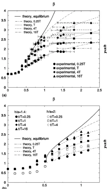
⫽0.25, 1, 4, 16, slowly converging to equilibrium separation ys(), plotted as a solid line.To compare this with experiments, the fine tuning of the time dependence requires a refined analysis of the hydrody-namic interactions in the above: since experiments are car-ried out in cells of width h comparable with the diameter a of the embedded holes—typically h/a lies between 1.1 and 2—a strong hydrodynamic coupling with the confining plates is present. Considering that both particles sit at a fixed frac-tion z of the plate separafrac-tion relative to the central posifrac-tion
共nonzero z can be obtained in principle between horizontal
plates due to the density contrast between the particles and ferrofluid兲, these interactions are represented according to Ref. 关37兴 by a normalization of the Stokes drag as
FIG. 5. Equilibrium separation distances as a function of the applied field for various ferrofluids.
/0⫽ f„a/共h⫹2zh兲…⫹ f „a/共h⫺2zh兲…⫺1, 共42兲
with0 the naked viscosity of the carrier ferrofluid, and
f共x兲⫽
冉
1⫺9x 16⫹ x3 8 ⫺ 45x4 256 ⫺ x5 16冊
⫺1 ⫹O共x6兲. 共43兲Two experimental cases will be considered here, where h/a
⫽1.4, z⯝0 and h/a⫽2, z⯝0.14, corresponding,
respec-tively, to /0⯝2.6 and 2.4. This is consistent with
Faucheux and Libchaber’s measures for a confined Brownian motion 关37兴 and with an experimental value /0⯝2.4,
which we measured in the h/a⫽1.4 case by placing 50m diameter particles between 70 m distant plates set up in vertical position, without any magnetic field, and by record-ing the motion of a srecord-ingle particle under the effect of buoy-ancy forces. The density of the ferrofluid was f⫽1.24 and the one of the polystyrene particles wasp⯝1. This value is slightly below the theoretical/0⯝2.6, which is consistent
with the effect of the Brownian motion of the particle along the normal direction, as analyzed in Ref.关37兴. We have cho-sen to use/0⫽2.5 in the following.
Hydrodynamic interactions between both particles were neglected, which should be a relatively poor approximation for particles close to contact, but become reasonable at sepa-rations x/h⬎2 where most of the time is spent to achieve equilibrium at relatively large separations, and is therefore the most important one in the present context. The typical magnitude of this error can be roughly estimated through the analyses performed by Dufresne et al. or Grier and Behrens
关21,38兴 for a close context: they derived for two particles of
diameter a, separated by x and at a distance h/2 from a single plate, the hydrodynamic corrections to the mobility to first order in x/a and x/h. Considering for simplicity a double contribution for two plates relative to Eq.共13兲 in Ref. 关21兴, contributions due to the particle-particle interactions become,
for h/a⫽1.4, x/h⬎2, less than 30% of the one due to the plates—term 9x/16 in Eq.共43兲.
We neglect also the rotational degrees of freedom of the ferrofluid itself, which can lead to the rotation of the non-magnetic spheres, and induce another type of hydrodynamic interactions between pairs of spheres: in ferrofluids submit-ted to circular magnetic fields, the rotation of the magnetite particles induces asymmetric stresses in the fluid, which leads to a counterrotation of the magnetic holes关2,23兴. The mismatch between this rotational motion of the magnetic holes and the one of the magnetites could in principle induce a vortex in the fluid flow around each of the holes, which would lead to a net hydrodynamic torque over close pairs of holes. Nonetheless, with the ferrofluid and field frequency regime used here共f⬍100 Hz兲, this rotational motion of the holes is so slow that it is hardly detectable. Experimentally, with a similar ferrofluid共kerosene-based,f⫽0.8兲, the hole’s frequency was bounded bys⬍0.01 Hz. This rotational mo-FIG. 6. Scaled separation as a function of time for various field
magnitudes and plate separations for ⫽H⬜/H储⫽0.8. The inset represents the same data for longer times.
FIG. 7. Separation as a function of time and for various field configurations, times, and cell sizes: merged data and theory.
tion was described theoretically in detail by Miguel and Rubi
关23兴. Through this theory, for the ferrofluid and field
frequen-cies used here, the frequency of the magnetic holes will straightforwardly be shown to be lower than s⬍0.05 Hz. This justifies for the present study the neglect of these rotation-induced hydrodynamic interactions. These interac-tions would in any case lead to a purely rotational motion of the hole pair, decoupled from the purely central forces in-duced by the magnetic interactions studied here. Experimen-tally, some very slow rotational motion of the hole pairs was indeed occasionally observed when the particles were close
共nonperiodic, angular velocity always lower than 0.001 Hz兲,
but no systematic trend for its direction or velocity was noted, i.e., this effect was beyond the experimental error.
To obtain the theoretical estimate of the hole’s frequency above, the Langevin parameter of the ferrofluid, defined关23兴 as ⫽m0H/kBT, where m0 is the magnetic moment of the
magnetites, is derived from the saturation magnetization of the ferrofluid and its susceptibility 关39兴 as ⫽3H/Msat.
For the ferrofluid used, ⫽1.9, Msat⫽200 G, H⫽14 Oe, and ⫽0.26. This enables us to express the ratio of the hole’s frequency over the field’s one as关23兴
s/f⫽⫺⌽共⫺tanh兲/共⫹tanh兲⫽⫺0.00041,
共44兲
where ⌽⫽⫺0.036 is the magnetite volume fraction of the ferrofluid. For the regimef⬍100 Hz where the experiments are carried, the sphere’s frequency is thus below s
⫽0.041 Hz.
B. Experimental results and scaling
We used pairs of a⫽50m diameter neutral polystyrene spheres of densityp⫽1, designed according to Ugelstad’s technique关40兴, and ferrofluids of susceptibilityf⫽1.9, den-sityf⫽1.24, and viscosity0⫽0.009 Pa s 关41兴, confined in
horizontal cells of thickness 70 m or 100m and width of the order of centimeters. The thickness of the cell was ob-tained by confining plates by quenching a few 70m diam-eter spheres between the two plates clamped together 共these spacers were typically half a centimeter distant from each other兲. The oscillating in-plane and constant normal field were generated by external coils, with a typical magnitude H储⫽H0⫽14.2 Oe, with frequencies from 10 to 100 Hz.
Magnitudes and phase of the field are accurate up to 1%, which also corresponds to the degree of homogeneity of the in- and out-of-plane fields throughout the entire cell. The direction of the constant field varies slightly along the cell, with a maximum 3° misalignment from the direction normal to the confining planes共these accuracies for the homogeneity and misalignment of the field were obtained directly by con-sidering the geometry of the Helmholtz coils generating the field, whose characteristic extent is 10 cm, together with a 0.5 mm accuracy for the position of the cell inside them兲. The in-plane motion of the particles was recorded using a microscope and a camera linked to a numerical data analysis setup. The entire experimental setup is described, for ex-ample, in Ref. 关12兴. The samples were prepared with a pure in-plane field to bring the particles in contact, after that the
in-plane field was maintained constant and the normal field was set to a constant H⬜e⫽(1⫹f)H储. The normal field required typically a few seconds to stabilize. Separation be-tween the particles were then recorded every 10 s, for 30 min. The concentration of the spheres in the entire sample was such that the nearest sphere or spacer would sit at least 20 diameters apart from the observed pair, which was suffi-ciently dilute not to influence the motion of the observed pair.
1. Time-dependent result at fixed field geometry and discussion The scaled separation as a function of time is shown in Fig. 6, for five experiments carried out at⫽0.8, i.e., for the potential represented in Fig. 3共c兲, which presents a single minimum at ys(0.8)⫽2.35. Four experiments were carried out in a h⫽70m thick cell, two of them at identical field amplitudes H储⫽H0⫽14.2 Oe and two other at H储⫽0.7H0;
0.5H0. The last experiment was carried out in a h
⫽100 m thick cell, with an in-plane field H0. These
pa-rameters corresponded, respectively, to characteristic times evaluated using Eq.共40兲 as T⫽32 s, 63 s, 129 s, and 192 s. a. Comparison with the theory. The large part of the figure represents the short-time evolution t⬍T 共typically the first minutes兲 and the encapsulated part shows longer time 共typi-cally 30 min兲. Every data point 共separated by 10 s兲 was used for the early regime, one point out of 2–12 depending on the experiment for the later one. At shorter times, the scaled data collapse reasonably well on the theoretical curve obtained from the theory sketched so far, solid line. The only two main outliers共first filled circle and triangle, t⫽10 s) presum-ably corresponded to a weaker normal field in the first few seconds, until it stabilized. For illustration, the first-order theory neglecting the magnetic confinement leads to the dot-dashed curve, obtained using Eq. 共41兲 with a bare potential retaining only the source-source term. This too simple theory clearly differs from data both at short and large times.
b. Corrections due to buoyancy. A third dashed theoretical curve was plotted, corresponding to a slightly refined calcu-lation of the interaction potential, where buoyancy forces due to the density contrast between ferrofluid and particles led to a shift z of the particle pairs from the central midplane of the cell. The relative displacement z/h due to this gravitational correction is evaluated in Sec. VII A as 15% in the weakest fields 0.5H0, h/a⫽1.4 case, and in the thicker layer H0, h/a⫽2 case, whereas it should remain around 6% for the thinner cells, higher field H0 case. The extended potential to
take this lateral shift into account is also derived in Sec. VII A, and the dashed curve corresponds to this potential at a fixed shift z/h⫽14%, which is the maximum possible in the thin cells, since it would correspond to contact of the par-ticles with one of the plates, coinciding with z/h⫽(1
⫺a/h)/2 at h/a⫽1.4. Considering this correction, one
would expect the diamond and squares to follow the dashed line, the circles to be close to the solid line, and the triangle to sit in between. This is indeed approximately the case at shorter times for the diamonds and rectangles, and the filled
circles fit well with the centered theory, both at short and long times. Nonetheless, it is worth noting that the open circles collapse rather with the lower field experiments than with the filled circles, another experiment carried with iden-tical parameters. This gives an estimate of the reproducibility of these experiments, corresponding roughly to a relative ex-perimental error bar of 10% for the separation at a given time, estimated between open and filled circle cases. The gravity-induced correction discussed above is of order 5% for the separation as a function of the dimensionless time, and the effect of this shift on the magnetic interactions can therefore hardly be distinguished from experimental disper-sion in terms of separation. Still, the renormalization of the time due to hydrodynamic interactions with the plates would lead in the thick cell case h/a⫽2 to/0⯝1.2 if the
par-ticles were considered as centered, z/h⫽0, instead of the value /0⫽2.5 that we used and corresponded to the
pre-dicted shift in that case, h/a⫽2, z/h⫽0.15. This gravity-induced correction is then clearly sensible for the hydrody-namic corrections, if not so much on the magnetic interactions, since the above incorrect viscositywould cor-respond to dividing T by 2, which would double the abscis-sas of the square data points and drive them way out of the theory and rest of the data. This shows qualitatively that this shift was indeed present in cases h/a⫽2, H0, and h/a
⫽1.4, 0.5H0, and that particles sat close to or in contact with
a plate in this last case.
c. Corrections due to experimental error on the field di-rections. The fourth dotted curve represents the theoretical effect of a misalignment of angle ␣⫽2.5° between the con-stant field and the normal direction. A direct generalization of Secs. II to IV to such configurations with a slightly tilted constant field shows that the time-averaged potential is still of the form in Eqs.共25兲 and 共26兲, with a modified parameter

⬘
⫽ H⬜e
共1⫹f兲关H储⫹
冑
2 sin共␣兲cos共兲H⬜ e兴⯝⫺
冑
2共1⫹f兲2sin共␣兲cos共兲, 共45兲 where is the angle between the projection of the constant field over the plane and the separation vector. This modified interaction potential leads to a torque tending to align the particle pair with the direction ⫽0, and a radial interac-tion force corresponding to a modified ⬘
in 关⫺冑
2(1⫹f)2sin(␣);兴,
⬘
decreasing with time towards the lower limit as the pair aligns with the in-plane constant component of the field. The dotted curve corresponds to this lower limit for a possible misalignment␣⫽2.5°, which is evaluated from the above as ⬘
⫽0.68.For the longer-time period shown in the encapsulated part of Fig. 6, an apparent equilibrium position was reached in each experiment after typically 6T—no more than a 1% rela-tive motion was noticed later when the experiments were conducted for several hours. This equilibrium separation cor-responds theoretically to the equilibrium one studied in the preceding section, ys(0.8)⫽2.35. The high field and thin cell experiments 共filled circles兲 agree well 共within 2%兲 with the theory with a purely normal field 共solid line兲, but
discrepan-cies between solid line and experiments are noticeable at longer times for the four other experiments. A comparison of the data with the dotted line shows that a misalignment of order 2.5° between constant field and normal direction is sufficient to explain these discrepancies: in these experi-ments, the particle pairs started at a relatively large angle from the in-plane component of the constant field, which is why the unmodified theory and experimental data are close for short times. At longer times, the particle pairs aligned with the direction ⫽0 and the modified theory 
⬘
⫽0.68 agree well with the data. An initial rotation of the particle pair and subsequent locking of this direction in a particular one was indeed observed in these experiments.Brownian motion in the ferrofluid can be proved to be entirely negligible for the relatively large particles and field we worked with, its relative magnitude compared to mag-netic interaction energy being kT/minU¯⭐kT/关A(d3/h3)min u兴
⯝10⫺4/min u⭐5⫻10⫺3 for the fields, particles, and plate separations considered here.
2. Scaled time-dependent results at various field geometries Experiments were carried out with in-plane field magni-tudes H0and normal fields jumping at initial time from 0 to
(1⫹f)H0with variousfrom 0 to 3.5. This was done for
a⫽50m diameter particles and plate separation h
⫽70m and 100 m. The results, scaled separation as a function of, at four values of the scaled time are shown in Fig. 7共a兲 for the thinner cell. The error bars correspond to a possible misalignment ␣⫽2.5° between the constant field and the normal direction: they represent the limits 关
⫺
冑
2(1⫹f)2sin(␣);兴 for the effective ⬘
parameter as explained in the preceding section. For the ‘‘c’’ regime ⬎c⫽1/
冑
2⬃0.7, theory and experiment agree well for any of the tested field parameters and times.The solid line represents the theoretical equilibrium value, studied in Sec. V. This is reached within typically 16T共8 min for h/a⫽1.4, H储⫽H0) for⭐1, or longer time at higher.
This is the main reason why the upward curvature of the theoretical solid curve at larger values ofis not observed in experimental data, which correspond to finite times, and for which other types of perturbations always enter the picture at very large times and distances.
In Fig. 7共b兲, we present the results of experiments carried out at two different plate separations, as a function of time and value of . The error bars have been omitted for read-ability, and the experimental points represented correspond to a constant field supposed purely normal关i.e., the abscissas are the upper limit of the error bars in Fig. 7共a兲兴. The experi-ments carried out in thicker cells, corresponding to weaker magnetic interaction forces, are more sensitive to any pertur-bations. The relative data collapse for both plate separations at 0.25 T and T when⬎cnonetheless show that the sepa-rations in this regime scale with plate separation, and not with particle diameter. Apart from the misalignment of the constant field with the normal direction, a possible source for these perturbations is as follows: when the particles come close to equilibrium, in-plane magnetic forces tend to zero, and the particle motion becomes more sensitive to any
inter-actions with the local environment 共confining plates兲—this being of course even more the case for weaker fields or larger h/a. There seems to be a pinning 共friction兲 of the particles to an absolute plate position at large times. The physical origin of this pinning is possibly due to roughness of the plates 共especially when particles are almost in con-tact兲, which can quench the particles through the magnetic perturbation due to this roughness 共the repulsion effect of a dipole by its images would make a particle sit preferably in positions of larger plate separation兲, or alternatively when particles are almost in contact with the plates can result in an in-plane component of the hydrodynamic coupling or contact forces responding to buoyancy forces. Instead of plate rough-ness, the same type of qualitative effects could be due to small impurities in the ferrofluids, starting to stick to the plates or particles at large times, when the chemical surfac-tant layers around large particles and possible impurities break apart in some points.
For the regime ⬍c, the simple theory presented here would predict that particles stay always in contact at y
⫽a/d⫽0.5 or 0.71 for ⬍m⬃0.55, and for m⬍⬍c would either stay in contact if a/h⬍yi() or go to the sec-ondary minimum ys() if yi()⬍a/h 共the separation be-tween the first and second case happening at ⫽0.61 for a/h⫽1/1.4 and ⫽0.67 for a/h⫽1/2). Particles seem in-deed to be in contact for⭐0.2, but start to separate signifi-cantly well before m. We note also that this separation seems grossly to be proportional to the particle diameter when ⭐0.3, where some finite separation can already be observed—ordinates of opened and filled symbols are mul-tiples of each other through a factor 100/70—and propor-tional to plate separation in the regime m⬍⬍c. This shows that an extra physical effect that was not taken into account here generated repulsive forces, whose range is finite but scales with the particle diameter. This effect suppresses then the short-range attraction in the regimem⬍⬍c, so that the particle jumps directly to ys(), which is always a stable minimum and not a metastable one. For ⬍m, this extra effect starts to separate the particles in proportion to particle diameter. The physical origin of this short-range re-pulsion should not be the particle-particle hydrodynamic in-teractions, which should slow down the relative motion rather than result in a net repulsion—see Refs. 关38,42兴. A probable candidate for this repulsion is rather the magnetic effect of the finite size of the spheres, particularly sensible when particles are close to contact. Even if an isolated non-magnetic sphere generates a purely dipolar perturbation when it is isolated in a homogeneous susceptible medium, this dipolar perturbation does not fulfill the boundary condi-tions along the surface of another magnetic sphere, suffi-ciently close of the first one to feel the heterogeneity of the perturbation at the scale of its diameter, which is naturally the case at a finite separation/diameter ratio. To model this short-range repulsion requires accounting for the magnetic perturbation generated by this nonpointlike character of close enough spherical particles. Though this can be performed by a simple image method for pairs of disks in 2D, one can show that this does not extend to pairs of spheres in 3D, and the proper mathematical description of this perturbation
re-quires the use of a series of spherical harmonics, which was not performed in the present study. To conclude this discus-sion, we note that this correction seems to be negligible at separations exceeding the sphere diameter x/a⬎2, as shows the agreement between experimental data and the present theory when⬎m.
Finally, we note that the present results are not contradic-tory with similar experiments carried out in Ref. 关2兴 with a slightly different ferrofluid, plate separation, and particle size, where it was reported that the equilibrium particle sepa-ration is approximately linear inonce the particles start to separate; for example, this is also the case with the present ferrofluid, in the particular case h/a⫽1.4 in the regime 0.3
⬍⬍1—see the filled triangles or theoretical curve in Fig.
7共a兲. This linear property is however shown here to be a mere coincidence, for this does not hold in the same  re-gime for h/a⫽2, or for any h/a when⬎1, where ys() is curved upwards, and any result y (,t) observed at a given finite time t is curved downwards.
VII. GENERALIZATION TO QUASI-2D SYSTEMS A. Gravity-induced corrections
Although the effect of the dipolar images in the confining plates tends to center particles at a midplane position, the density contrast between the ferrofluid and particles tends to drive the particle out of it for large enough particles. An estimation of this effect can be obtained by considering for each particle the sole effect of its own images plus buoyancy forces—for the simple estimation we look at here, we will neglect the coupling between one source and the images of the other. Extending the analysis performed in Secs. III and IV A to a single dipole lying at a vertical distance z from the center between two horizontal plates, we directly have
U¯shifted共z兲⫽Aa 3 h3u shifted
冉
z h冊
, 共46兲 ushifted共s兲⫽兺
l苸Z* 兩l兩 1⫺2共⫺1兲 l2 兩l⫺关1⫹共⫺1兲l⫹1兴s兩3. 共47兲This potential can be shown to be always centering for any value of , i.e., to have a single minimum in s⫽0 and to diverge to infinity at s⫽⫾0.5—plate contact for very small particles. Equilibrium between gravity forces and magnetic interactions between the dipole and its images leads to
dU¯shifted dz ⫽V共g⫺f兲, 共48兲 i.e., du ds⫽ 48共g⫺f兲gh f¯2H储2 h3 d3. 共49兲
For small separations 共i.e, small particles or strong enough fields兲, a Taylor expansion to first order around the plates’ center gives
du ds⫽96C共兲共1⫹2 2兲兩s兩, 共50兲 C共兲⫽
兺
n苸N 2n⫹1/共2n⫹1兲5, 共51兲which is valid up to 25% for s⬍0.1. Thus, the displacement looked for can be evaluated as
s⫽z/a⫽ 共g⫺f兲gh
2C共兲共1⫹22兲f¯2H储2 h3
a3 共52兲 when this quantity does not exceed 0.1, or directly using Eqs.共49兲 and 共50兲 otherwise. For the ferrofluid and particles we used, this led, respectively, for h⫽70m, H储
⫽H0, 0.7 H0, or 0.5 H0 and h⫽100m, H储⫽H0 to s
⫽0.06, 0.10, 0.15, and 0.15.
The magnetic interaction potentials were unaffected up to 1% in the s⫽0.06 vertical shift case, and the dashed curve in Fig. 6 was obtained by considering particles at a fixed s
⫽0.14 out-of-midplane shift, using a generalized potential
obtained for a configuration sketched in Fig. 8 through an extension of the method used in Secs. III and IV A as
uspair共y兲⫽共22⫺1兲y⫺3⫹4
兺
l⫽1 ⫹⬁ l冉
1⫹共⫺1兲 l2 关y2⫹m s共l兲2兴3/2 ⫺3 2 y2⫹2共⫺1兲lms共l兲22 关y2⫹m s共l兲2兴5/2冊
, 共53兲 ms共l兲⫽l⫹s关1⫹共⫺1兲l兴. 共54兲This s⫽0.14 value was picked to represent the magnetic effect of a shift sufficient to bring particles in contact with the plates in the h/a⫽1.4, 0.5 H0 case. To an accuracy of
1%, the results for s⫽0.15 were very close to this case, the ones for s⫽0.06 very close to pure in-plane situations, and the situation s⫽0.10 fell roughly halfway between both, and were therefore omitted from Fig. 6 for readability.
B. Stability of the plane solutions and buckled configurations
When particles are sufficiently small or fields sufficiently high, the preceding section establishes that the confining plates have an effective repulsive effect on an isolated particle, which is therefore centered on midplane. In the case of a pair of particles, the interactions between one source and the images of the other one might nonetheless modify that picture and make the plane solutions described in this paper unstable, as have been observed in some experiments. Ne-glecting gravity, we will here generalize the interaction
potential to configurations where particle pairs are allowed to tilt on both sides of the midplane, i.e., where both are displaced by the same distance z on both sides of it—cf. Fig. 9. We consider only symmetric situations due to the sym-metry of the problem under parity in the absence of gravi-tational forces. The effective interaction potential is ob-tained similar to the plane one, and comes as U¯ (x,z)
⫽A(a3/h3)u(x/h,z/h), where
u共y,s兲⫽2
兺
l⫽⫺⬁ ⫹⬁ 兩l兩冉
1⫹共⫺1兲l2 关y2⫹共l⫹p ls兲2兴3/2 ⫺32 y 2⫹2共⫺1兲l共l⫹p ls兲22 关y2⫹共l⫹p ls兲2兴5/2冊
⫹2兺
l苸Z* 兩l兩关1⫺2共⫺1兲l2兴 ⫻冉
1 兩l⫹共2⫺pl兲s兩3 ⫺ 1 兩l兩3冊
, 共55兲 pl⫽1⫹共⫺1兲l, 共56兲which reduces to the previous in-plane solution, Eq. 共28兲, when s⫽0. Contour plots of this pair potential are displayed in Fig. 10 for the ferrofluid used here,f⫽1.9, and the four types of potentials, ⫺ values, are identical to the ones adopted in Sec. IV B. Black and white represent, respec-tively, u⫽⫺0.2 and 0.5 in panels 共a兲 and 共b兲, u⫽⫺0.2 and 1 in 共c兲 and 共d兲, and the gray level linear in u in between. Out-of-plane values represented cover the whole possible range 0⭐s⭐0.5 in 共c兲 and 共d兲, and are restricted to 10% from the midplane in共a兲 and 共b兲. The in-plane configurations correspond to the bottom axis of those graphs.
In-plane solutions are in principle locally stable if 2u/s2( y ,0)⬎0, otherwise particle pairs will tend to tilt.
For both first cases,⬍c, we note that2u/s2⬎0 for any possible (y ,s), and any tilt is restored by the magnetic image effect; the plane configurations are indeed stable. As soon as ⬎c, besides the minima (y ,s)⫽(ys,0) or (⫹⬁,0) in 共c兲 or 共d兲 case, another local minimum appears at a certain (y ,s)⫽„0,se()…: particles can be stable at a finite distance on top of each other—the pair tends to align with the large normal field— or if they are close enough to be attracted by this potential minimum but too large 关a⬎se() and a
⬎h/2], contact forces between them and with the confining
plates will attract them to a buckled configuration where both particles are in contact with each other, and with one differ-ent plate each. Note that 0⬍se()⬍0.5, i.e., very small par-ticles, aⰆh, at this second minimum would sit on top of each other, neither in contact between them nor with the
plates. The criterion to determine whether particles are at-tracted by the in-plane solution, or the buckled configura-tions, is to determine whether the present (y ,s) lie in the basin of attraction of one minimum or the other. Both basins of attraction are separated by a ridge of the potential, on which u decreases under the effect of any perturbation of ( y ,s) apart from the ones directed exactly along its gradient. This boundary between both basins of attraction, noted yl(s,), was determined numerically and plotted as the gray solid line in Figs. 10共c兲 and 10共d兲. We note that the whole axis ( y ,0) lies in the basin of attraction of the plane mini-mum, so any particle pair starting with no tilt should end up so. However, at short enough distances y in a c field, or at any in-plane distance in a d field, certain configurations with a finite tilt are attracted by the normal-aligned pair minimum, and will end up in a buckled contact configuration or normal-aligned pair. We have determined for every the maximum
ym()⫽maxsyl(s,). For a given , when y⬎ym(), any tilted configuration will be attracted by the in-plane solution, whereas for certain finite tilts at close enough y⬍ym(), the pairs will be attracted towards buckled in-contact configura-tions. The function ym() is displayed as the dashed curve in Fig. 11—the solid curve is a reminder of the equilibrium in-plane distances ys(),yi() determined in Sec. V. The function ym() diverges when→u⫺, illustrating the fact that in any d-type field, configurations with out-of-plane tilts s close to 0.5, i.e., both particle centers almost along the plates 共for small enough particles兲 will be attracted by the normal-aligned pair mode.
This effect is believed to be responsible for the lattices of buckled chains of particles in contact observed in Ref. 关8兴. These were observed in pure normal fields共⫽⫹⬁兲, and the nontrivial character of the lattices, being hexagonal or square instead of triangular lattices characteristic of attractive
actions at any range, can be qualitatively explained by frus-tration effects: neighboring particles tend to sit in top-down contact configurations, but top-top or down-down configura-tions are repulsive—cf. shifted potential developed in the preceding section—and therefore lattices with noneven num-ber of particles along the loops, as the triangular one, are disfavored in comparison with those involving even numbers in loops, such as the square or hexagonal ones.
Eventually, the local stability of a plane configuration was investigated in fields of c or d type: the second derivative 2u/s2 is positive at s⫽0 for large enough distances, and
small out-of-plane tilts will be restored by magnetic interac-tions, but below a certain y⬍yp(), 2u/s2( y ,s⫽0)⬍0, and the in-plane solution will be locally unstable. However, the preceding section established that this out-of-plane char-acter will be transient, since this case will still be attracted at long times by the in-plane solution. This upper limit yp() below which in-plane configurations will go to a transient out-of-plane regime was determined numerically for any  and plotted as the dash-dot curve in Fig. 11.
VIII. CONCLUSIONS
For pairs of magnetic holes in ferrofluid layers of finite thickness, exposed to fast oscillating conic magnetic fields,
we have established the effective interaction potential driv-ing their slow motion. The importance of the magnetic per-meability contrast between ferrofluid and confining plates on these interactions was demonstrated, and the resulting pair potential analytically derived. This allowed the classification of those interaction potentials into four types, two of which present a secondary minimum at a finite distance. A simple finite-time theory for these non-Brownian microspheres, in-cluding the hydrodynamic interactions of the holes with the confining plates, was directly compared and confirmed by experimental results, through data collapse of the scaled separation as a function of scaled time, for various plate separations and field magnitudes. The relaxation time of these systems to reach equilibrium when there is any was typically a few minutes or above. Eventually, we generalized the study to full three dimensions in the layer thickness, and studied the stability of the in-plane configurations. This es-tablished that although in-plane configurations are stable at small normal fields, or at large ones and sufficient particle separation, hole pairs can be attracted by another stable con-figuration of tilted pairs of particles with contact between them and contact with one plate each.
This simple theory renders for so far unexplained ob-served configurations of magnetic holes, namely, 2D lattices with finite separation or buckled lattices of tilted pairs of particles. In principle, the effect described here in detail should be important in any colloidal system confined in a layer with significant magnetic permeability or dielectric contrast between the fluid and confining structure.
The ability to tune the equilibrium distance at will through the ratio of the normal over in-plane magnitude of the external field makes this magnetic hole system a good candidate for various applications, such as the manipulation of large molecules using the magnetic holes, for example, proteins which would be fixed to one or several holes coated with antigens, the determination of the transport properties of a ferrofluid, or as analog model of systems implying discrete particles of tunable interactions and hydrodynamic coupling to the carrier fluid. The effective pair interactions derived here should be a fundamental brick of any such applications.
关1兴 A.T. Skjeltorp, Phys. Rev. Lett. 51, 2306 共1983兲.
关2兴 G. Helgesen and A.T. Skjeltorp, J. Magn. Magn. Mater. 97, 25 共1991兲.
关3兴 A.T. Skjeltorp, J. Magn. Magn. Mater. 37, 253 共1983兲. 关4兴 A.T. Skjeltorp, J. Appl. Phys. 55, 2587 共1984兲. 关5兴 A.T. Skjeltorp, Physica B & C 127, 411 共1984兲. 关6兴 A.T. Skjeltorp, Physica A 213, 30 共1995兲. 关7兴 A.T. Skjeltorp, J. Appl. Phys. 57, 3285 共1985兲.
关8兴 A.T. Skjeltorp and G. Helgesen, Physica A 176, 37 共1991兲. 关9兴 G. Helgesen and A.T. Skjeltorp, Physica A 170, 488 共1991兲. 关10兴 G. Helgesen, P. Pieranski, and A.T. Skjeltorp, Phys. Rev. Lett.
64, 1425共1990兲.
关11兴 G. Helgesen, P. Pieranski, and A.T. Skjeltorp, Phys. Rev. A 42,
7271共1990兲.
关12兴 G. Helgesen and A.T. Skjeltorp, J. Appl. Phys. 69, 8277 共1991兲.
关13兴 M.C. Miguel and J.M. Rubi, Physica A 231, 288 共1996兲. 关14兴 A.T. Skjeltorp, S. Clausen, and G. Helgesen, J. Magn. Magn.
Mater. 226, 534共2001兲.
关15兴 A.T. Skjeltorp, S. Clausen, and G. Helgesen, Physica A 274,
267共1999兲.
关16兴 S. Clausen, G. Helgesen, and A.T. Skjeltorp, Int. J. Bifurcation
Chaos Appl. Sci. Eng. 8, 1383共1998兲.
关17兴 S. Clausen, G. Helgesen, and A.T. Skjeltorp, Phys. Rev. E 58,
4229共1998兲.
关18兴 P. Pieranski, S. Clausen, G. Helgesen, and A.T. Skjeltorp,
Phys. Rev. Lett. 77, 1620共1996兲.
关19兴 G. Helgesen, A.T. Skjeltorp, P.M. Mors, R. Botet, and R.
Jul-lien, Phys. Rev. Lett. 61, 1736共1988兲.
关20兴 M. Warner and R. Hornreich, J. Phys. A 18, 2325 共1985兲. 关21兴 P. Davies, J. Popplewell, G. Martin, A. Bradbury, and R.
Chantrell, J. Phys. D 19, 469共1986兲.