Assessment of one year of high-resolution operational forecasts for the southeastern Mediterranean shelf region in the MFSTEP project

(1)

HAL Id: hal-00298459

https://hal.archives-ouvertes.fr/hal-00298459

Submitted on 18 Dec 2006

HAL is a multi-disciplinary open access

archive for the deposit and dissemination of sci-entific research documents, whether they are pub-lished or not. The documents may come from teaching and research institutions in France or abroad, or from public or private research centers.

L’archive ouverte pluridisciplinaire HAL, est destinée au dépôt et à la diffusion de documents scientifiques de niveau recherche, publiés ou non, émanant des établissements d’enseignement et de recherche français ou étrangers, des laboratoires publics ou privés.

Assessment of one year of high-resolution operational

forecasts for the southeastern Mediterranean shelf

region in the MFSTEP project

S. Brenner, A. Murashkovsky, I. Gertman

To cite this version:

S. Brenner, A. Murashkovsky, I. Gertman. Assessment of one year of high-resolution operational forecasts for the southeastern Mediterranean shelf region in the MFSTEP project. Ocean Science Discussions, European Geosciences Union, 2006, 3 (6), pp.2059-2085. �hal-00298459�

(2)

OSD

3, 2059–2085, 2006

Operational forecasts for the southeastern

Mediterranean S. Brenner et al. Title Page Abstract Introduction Conclusions References Tables Figures ◭ ◮ ◭ ◮ Back Close

Full Screen / Esc

Printer-friendly Version Interactive Discussion

EGU

Ocean Sci. Discuss., 3, 2059–2085, 2006 www.ocean-sci-discuss.net/3/2059/2006/ © Author(s) 2006. This work is licensed under a Creative Commons License.

Ocean Science Discussions

Papers published in Ocean Science Discussions are under open-access review for the journal Ocean Science

Assessment of one year of

high-resolution operational forecasts for

the southeastern Mediterranean shelf

region in the MFSTEP project

S. Brenner1,2, A. Murashkovsky2, and I. Gertman2 1

Department of Geography and Environment, Bar Ilan University, Ramat Gan 52900, Israel

2

National Institute of Oceanography, Israel Oceanographic and Limnological Research, PO Box 8030, Haifa 31080, Israel

Received: 5 October 2006 – Accepted: 1 December 2006 – Published: 18 December 2006 Correspondence to: S. Brenner (sbrenner@mail.biu.ac.il)

(3)

OSD

3, 2059–2085, 2006

Full Screen / Esc

EGU Abstract

Within the framework of the MFSTEP project an operational ocean forecasting system for the Southeastern Mediterranean Sea has been implemented and evaluated through a series of preoperational tests and subsequently for one year of operational forecasts. The system is based on the Princeton Ocean Model (POM). The high-resolution shelf

5

model is nested in a coarser resolution regional model, which is in turn nested in a coarser resolution full Mediterranean model. The respective grid sizes of the three models are 1.25, 3, and 6 km. Lateral boundary conditions are taken from the daily mean fields of the regional model while the surface forcing is taken from the hourly values of a regional atmospheric forecast model. When compared to satellite derived

10

sea surface temperatures and the MFSTEP analysis fields, the high-resolution shelf model forecasts are significantly more skillful than the coarser model forecasts for the relevant domain. In the four-day forecasts, most of the error appears to be due to the analysis error inherent in the initial conditions. Future development of the system will therefore focus on improving the specification of the initial conditions.

15

1 Introduction

During the past 25–30 years scientific interest in the oceanography of the Mediter-ranean Sea in general, and the Eastern MediterMediter-ranean in particular, was renewed for various reasons. As a result, in the early 1980’s several intensive regional and inter-national fields campaigns were designed to investigate the circulation. Most notable

20

among these were the Marine Climate (MC) program (Hecht et al., 1988; Robinson et al., 1987) and the Physical Oceanography of the Eastern Mediterranean (POEM) program (POEM Group, 1992). In the former, analysis of the data from 28 cruises conducted over a five year period in the region south of Cyprus showed for the first time that the circulation in the eastern Levantine basin was characterized by a highly

25

(4)

OSD

3, 2059–2085, 2006

Full Screen / Esc

EGU

multinational cruises conducted over a period of ten years showed that the general circulation of the entire Eastern Mediterranean was energetic and variable on scales ranging from a basinwide thermohaline cell, driven by deep water formation in the Adriatic, to mesoscale eddies. Further analysis of the POEM data and data from later cruises also revealed a major transition in the deep and intermediate water circulation

5

(e.g., Malanotte-Rizzoli, et al., 1999) driven by a switch in the primary source of deep water formation from the Adriatic to the Aegean (Klein et al., 1999).

Following the new description of the circulation that emerged from these programs, various numerical models were applied to the Mediterranean to further investigate the processes that drive the circulation. Low resolution (roughly 25 km horizontal grid

spac-10

ing and 19 vertical levels or less), basinwide models such as Roussenov et al. (1995), Zavatarelli and Mellor (1995), and Wu and Haines (1998) were used to study the cli-matological mean circulation of the entire Mediterranean. Other models focused on particular process studies and/or the sub-basin circulation. For example, Korres et al. (2000a,b) used the same model as Roussenov et al. (1995) but with increased vertical

15

resolution and improved surface forcing in order to study the response of the general circulation to interannual atmospheric variability. Wu et al. (2000) increased the hori-zontal resolution of the model of Wu and Haines (1998), but used highly simplified sur-face forcing parameterization in order to study the process of deep-water formation in the Eastern Mediterranean. Finally, Lascaratos and Nittis (1998) used an intermediate

20

resolution, eddy-resolving (5.5 km grid) model of the Levantine and southern Aegean Seas to study the process of intermediate water formation. While this list is of modeling studies is very partial, it does indicate the wide interest in studying the circulation of the Mediterranean.

As the data and research models provided new understanding of the circulation, and

25

as observational systems and computer technology advanced, by the late 1990’s it was decided to apply this new knowledge to the problem of operational ocean forecasting. By an operational forecasting system we refer to one in which analyzed and predicted fields are routinely, and automatically, made available in near real time at regular

(5)

in-OSD

3, 2059–2085, 2006

Full Screen / Esc

EGU

tervals. By necessity, the activities required for a fully operational system include data collection and capture; spatiotemporal analysis (i.e., data assimilation) to provide grid-ded, three dimensional maps of the requisite parameters to fully describe the synoptic mass and motion fields; and predictions for various forecast lead times. All of this must of course be done within a reasonable amount of time in order to make the forecasts

5

useful.

Successful computer based atmospheric forecasting was first introduced over forty years ago. Since then a clear emphasis has been placed on: (i) the development of improved, more complex, and more accurate models; (ii) the development of data as-similation systems which strive to produce a more precise set of initial conditions from

10

the observations: and (iii) the design and deployment of more accurate and compre-hensive observational networks. For various reasons, operational ocean forecasting has lagged behind its meteorological counterpart and has only seen rapid develop-ment over the past 10–15 years, with the exception of surface wave forecasting, which has a longer history, due in part to its close connection to meteorological prediction

15

and its requirement for fewer external data (i.e., only surface winds). Research and development in ocean hydrodynamic forecasting has followed an approach similar to atmospheric forecasting in terms of model development and data collection. One of the major limitations from the oceanic point of view is the scarcity of field data needed to produce three-dimensional initial conditions and verification fields. This has led to new

20

challenges, especially in data assimilation, not faced by meteorologists. For example, remotely sensed measurements of sea surface temperature and sea surface height routinely provide nearly synoptic coverage of large parts of the oceans and seas, but the data are limited to the near surface layer. In the absence of dedicated hydrographic cruises, which tend to be slow and relatively expensive, crucial subsurface data, and

25

even surface salinity, are only partially observed through ships of opportunity cruises (e.g., Manzella et al., 2003) or indirectly inferred through various feature models (Glenn et al., 1990) or statistical relationships (e.g., Ezer and Mellor, 1994).

(6)

OSD

3, 2059–2085, 2006

Full Screen / Esc

EGU

requires the resources of a major center (a large meteorological service or a dedi-cated ocean forecasting center), the rapid development and widespread availability of relatively inexpensive workstations has made quasi-operational to operational regional forecasting capabilities accessible to many smaller forecasting and/or research centers with only modest resources. This of course depends on the availability of coarser grid

5

large-scale forecasts, data fields, and atmospheric forecasts from the larger forecasting centers. Many major centers provide such services today for large parts of the world ocean. Some examples of ocean-forecasting centers or programs with an emphasis on the European seas include (nonexhaustive list): the UK Met Office FOAM system (Met Office, 2006); MERCATOR forecasts (MERCATOR, 2006); and the Mediterranean

10

Forecasting System Pilot Project (MFSPP; Pinardi et al., 2003), or more recently, the Mediterranean Forecasting System Towards Environmental Prediction (MFSTEP, 2003) specifically for the Mediterranean. Atmospheric forecasts needed to drive the ocean forecasts are available globally from various centers such as the National Cen-ter for Environmental Prediction (NCEP, Washington), the UK Met Office, the European

15

Centre for Medium Range Weather Forecasts (ECMWF) and regionally from various local meteorological services and/or research centers.

The purpose of this paper is to present the implementation and assessment of the performance of one of the regional components of an operational hydrodynamic forecasting system, within the context of participation in the larger, multinational

pro-20

gram MFSTEP to develop a complete forecasting system for the entire Mediterranean Sea. Since 15 June 2005, hydrodynamic forecasts for the southeastern corner of the Mediterranean Sea with a four-day lead-time are run once per week and posted on the Internet for dissemination and public use. The clear focus here is to run the forecast model, while only a limited amount of data is collected for forecast verification. Since a

25

systematic regional data collection program has not yet been implemented, no signifi-cant effort has been made to run a local data assimilation system. It is assumed that the necessary gridded fields for forcing, initial, and lateral boundary conditions are, and will continue to be available from other forecast centers.

(7)

OSD

3, 2059–2085, 2006

Full Screen / Esc

EGU

In Sect. 2 we describe the hydrodynamic model and its implementation within the context of MFSTEP. In Sect. 3 we present a preliminary assessment of the model performance and forecast skill for one full year of weekly forecasts. Our conclusions and recommendations are presented in Sect. 4.

2 Model description and setup

5

Within the framework of several international and local projects, we have developed and refined a modeling system that is capable of providing high-resolution, operational predictions of the temperature, salinity, currents, and free surface height in various parts of the eastern Mediterranean Sea. Since we are interested in focusing on spe-cific regions, by necessity the model must be nested into a coarser resolution, larger

10

scale model. The concept of nesting numerical models for the purpose of zooming and refining the forecasts for smaller regions originated in the field of numerical weather prediction over thirty years ago. The major challenge in designing the nesting proce-dure is to specify lateral boundary conditions that are stable and robust and that allow for accurate simulations in the high-resolution model domain without causing adverse

15

boundary affects. Unfortunately, there is no unique approach that is applicable to all situations and quite often the nesting methodology must be developed on a case-by-case basis. Nevertheless, two general rules do apply. First, the more that is known about the coarse domain (spatially and temporally) the better the nested simulation will be. Second, the boundary conditions at outflow points must allow information to

20

freely advect out of the high-resolution domain with no reflection at the boundary (e.g., Orlanski, 1976).

Initially this work was conducted within the framework MFSPP (Pinardi et al., 2003), where we designed and tested a high-resolution nested model for the southeastern shelf region of the Levantine Basin (Brenner, 2003a) as part of a prototype operational

25

forecasting system for the entire Mediterranean Sea with multi-nested models. The main purpose there was to demonstrate the viability of the prototype system in general,

(8)

OSD

3, 2059–2085, 2006

Full Screen / Esc

EGU

and the accuracy and robustness of the nesting procedure. During the course of MF-SPP, various other projects came up which also required the use of a high-resolution, nested model in other sub regions of the Levantine Basin. It soon became clear that by automating, to the extent possible, the process of model setup we would have an extremely useful tool that could be quickly and easily applied to various problems and

5

situations. Thus we had the need to develop a relocatable, nested model (Brenner, 2003b). In order to apply the model to a specific region three basic steps must be ex-ecuted: (a) defining the domain, grid, and bathymetry, (b) preparing the time series of lateral and surface boundary conditions, and (c) running the simulation or forecast. The success of this strategy depends upon two main factors: (a) specification of a nesting

10

procedure that is robust (i.e., limited selection of lateral boundary conditions), and (b) limiting the number of sources of lateral boundary conditions and surface forcing. A general overview of some of these applications is given in Brenner et al. (2006). Here we focus on MFSTEP, which is the one particular application that has been running in a near real-time operational mode since June 2005.

15

2.1 General model description, lateral boundary conditions, and surface forcing As with many of the other MFSTEP partners running regional and shelf models, we have chosen to use the Princeton Ocean Model (POM), which is a three-dimensional, time dependent, free surface, primitive equations model, including full thermodynam-ics, that uses a terrain following (sigma) vertical coordinate (Blumberg and Mellor,

20

1987). It also contains an imbedded level 2.5 turbulence closure model based on Mellor and Yamada (1982). The prognostic variables in the model are the two horizon-tal components of momentum, potential temperature, salinity, the free surface height, the turbulent kinetic energy, and the turbulence macroscale. The diagnostic equa-tions needed to close the system include the hydrostatic equation, and the equation of

25

state (in the form proposed by Mellor, 1991). The sigma vertical velocity is deduced from mass continuity. Removing a domain mean, hydrostatic pressure field reduces the pressure gradient errors associated with the sigma coordinate over steep

(9)

topog-OSD

3, 2059–2085, 2006

Full Screen / Esc

EGU

raphy (Mellor et al., 1994). Spatial differencing is second order accurate and uses an Arakawa C grid. The time integration uses a split explicit method in which the barotropic and baroclinic velocities are integrated separately with different size time steps.

After extensive experimentation with our model we found a single set of open bound-ary conditions for one-way nesting that seems to be robust and works well for all of

5

the applications of the model in our region including the present MFSTEP shelf model (Brenner et al., 2006). The boundary conditions used allow information to freely pass into and out of our domain with no apparent adverse effects such as reflection or noise along the open boundaries. Other partners of MFSPP adopted similar boundary con-ditions. For each vertical layer, the normal and tangential components of the total

10

(baroclinic + barotropic) velocity are bilinearly interpolated from the coarse grid to the fine grid. Thus

(UPOM, VPOM)=(UCOARSE, VCOARSE) (1)

where U and V are the normal and tangential components, respectively and the sub-scripts POM and COARSE refer to the shelf model and the driving model, respectively.

15

Components of the barotropic velocity are also bilinearly interpolated form the coarse grid. However this was found to quickly lead to a numerical instability, which we were able to control by adding a weak gravity wave radiation term to the normal component. Thus the normal component is given by

¯

UPOM= ¯UCOARSE+ε

r g

H (ζPOM−ζCOARSE) (2)

20

where the overbar stands for the barotropic (depth averaged) velocity, ε provides the relative direction of the outward propagating wave according to ε=1 on the northern boundary and –1 on the western boundary, g is gravity, H is the water depth, and ζ is the free surface. The tangential component is given by

VPOM=VCOARSE (3)

(10)

OSD

3, 2059–2085, 2006

Full Screen / Esc

EGU

In addition, the bathymetry along the open boundaries is adjusted to agree with the bathymetry of the coarse grid and an integral constraint is imposed so that the net normal coarse grid transport across the boundary is preserved on the fine grid. It should also be noted that the bathymetry on both grids is derived from the same initial data set. Further details can be found in Brenner (2003b).

5

At inflow points tracers (temperature and salinity) are bilinearly interpolated from the coarse grid while at outflow points the values are extrapolated from the first interior grid point using an upstream advection equation of the form

∂T

∂t+U

∂T

∂x=0 (4)

where T represents the tracer, t is time, U is the normal component of velocity, and x

10

the normal coordinate. This is applied to each vertical layer individually.

In addition to the lateral boundary conditions, the model requires surface forcing from the atmosphere. The necessary fields include the two components of the wind stress for the momentum and turbulent kinetic energy equations, the four components of the surface heat flux (shortwave heating, longwave cooling, latent heat flux, and sensible

15

heat flux) for the thermodynamic equation, and the freshwater flux (evaporation – pre-cipitation) for the salinity equation. Either climatological data or an atmospheric fore-cast model provides all of these. In this configuration, Brenner (2003a) found that for the MFSPP multiyear, climatologically forced, nested simulations of the southeastern shelf region the model exhibited long-term (multiyear) stability. For other applications

20

with shorter duration simulations, Brenner et al. (2006) also found the model to be well behaved with these boundary conditions and forcing.

2.2 MFSTEP Southeastern Levantine shelf model

The domain of the present model is the southeastern corner of the Levantine Basin covering a region 188 km wide and 282 km long with open boundaries along the

north-25

(11)

OSD

3, 2059–2085, 2006

Full Screen / Esc

EGU

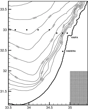
to the model grid from the 1’ resolution US Navy DBDB5 gridded data set. The domain and bathymetry are shown in Fig. 1. The dots in the figure indicate the locations of the various field measurements that are used for the forecast verification (see below). Coarse grid lateral boundary data were taken from the corresponding forecasts of the regional model, ALERMO, described by Korres and Lascaratos (2003). In a previous

5

study, Brenner (2003a) showed that the main advantages of the higher resolution shelf model were: better coverage of the shallow region, which is not adequately resolved by the driving model; a more sharply defined coastal jet; and generation of a more energetic small-scale eddy field. For MFSTEP we retained the same domain as in Brenner (2003a), but the horizontal grid spacing was reduced from 2 to 1.25 km. The

10

number of vertical sigma layers has been reduced from 30 to 25 corresponding to the change made in the MFSTEP version of ALERMO. A portion of the grid (every second point) is shown in the lower right corner of Fig. 1.

This version of the model was initially tested as part of the preoperational checkout phase of MFSTEP in two steps. The first period, referred to as the Special Validation

15

Period (SVP), was selected as the entire month of Jan 2003. The higher resolution MFSTEP version of ALERMO (3 km grid spacing) was run at the University of Athens using initial and lateral boundary conditions taken from the full Mediterranean MFSTEP model (OGCM) and surface forcing based on the atmospheric forecasts form the re-gional model SKIRON, which is also run at the University of Athens and provided as

20

part of the MFSTEP suite of products. ALERMO was run for thirty consecutive days, from which we extracted our initial conditions and lateral boundary conditions. We also used the same daily SKIRON forcing. Both models successfully reproduce the well-known northward flowing current over the continental shelf and slope (Rosentraub and Brenner, 2006), while the main advantage of the shelf model was to provide a better

25

and more detailed definition of the shelf circulation. Also no noise or spurious boundary effects appeared even though the forcing had much higher temporal resolution than in the previous MFSPP climatological simulations. Further details are given in Brenner et al. (2006).

(12)

OSD

3, 2059–2085, 2006

Full Screen / Esc

EGU

The second step in the preoperational testing of MFSTEP was conducted during the Targeted Operational Period (TOP) from September 2004 through February 2005. During the TOP, data (satellite based sea surface temperature and sea surface height, XBT temperature profiles, and drifters) were collected on a regular basis and the Mediterranean-wide data assimilation system and all forecast models (i.e., the full

5

Mediterranean model, OGCM, as well as the nested regional and shelf models) were run in a quasi-operational mode once per week. In our case, a four-day forecast was run once per week with initial and lateral boundary conditions provided by the corre-sponding daily mean forecast fields from ALERMO while surface forcing was provided by the daily mean SKIRON atmospheric forecasts. Brenner et al. (2006) showed that

10

for all forecast lead times the shelf model predicted SST is more skillful than the coarser resolution model, and both models beat persistence of the initial conditions.

3 Skill assessment of operational forecasts

In view of the encouraging results from the preoperational checks, we began to run the model in an operational mode on 15 June 2005, producing a four-day forecast once per

15

week. The forecasts are posted on the web athttp://isramar.ocean.org.il/ShelfModel/. To further expand our assessment of the forecast skill of the model, we have selected a one year period from Dec 2004 − Dec 2005 which consists of the second half of the MFSTEP TOP followed by three months of continued preoperational runs and the first six months of our operational system. In all cases, the daily mean ALERMO fields

pro-20

vided the lateral boundary conditions while the atmospheric forcing was taken from the hourly forecasts of SKIRON (as compared to the daily mean fields used in the original TOP phase). For the 48 forecasts available during this period we compared the pre-dicted SST fields with the SST fields from the MFSTEP hindcasts analyses and with daily satellite SST fields, which were also provided through MFSTEP. For the forecast

25

skill metrics we use the root mean square error (RMSE) and the anomaly correlation coefficient (ACC) (see for example, Robinson et al., 2002; Rowley et al., 2002). The

(13)

OSD

3, 2059–2085, 2006

Full Screen / Esc

EGU

former provides information on the typical magnitude of the forecast error while the lat-ter is indicative of the model’s ability to predict the spatial patlat-terns of SST anomalies. We also compare the forecasts to measurements from a single point current meter lo-cated near Hadera and to CTD measurements conducted along an east-west transect extending seaward from Haifa. The data points are indicated by the dots in Fig. 1.

5

3.1 Comparison to satellite observed SST and MFSTEP analyses

In terms of observations, the data set that has the best spatial and temporal cover-age consists of the gridded analyses of satellite based sea surface temperatures that are produced within the framework of MFSTEP. These fields are available daily on a uniform 1/16◦ _{grid (approximately 6 km). The other regularly available data set}

con-10

sists of the MFSTEP daily analyses (sometimes referred to as hindcasts) of the full three-dimensional ocean fields produced by the full Mediterranean data assimilation system. The data assimilated by this system on a regular basis include the satellite SST and sea surface height (altimeter), and temperature and salinity profiles from sub-surface drifters. When available, temperature profiles from XBTs collected by ships of

15

opportunity are also assimilated. Further details can be found on the MFSTEP web site.

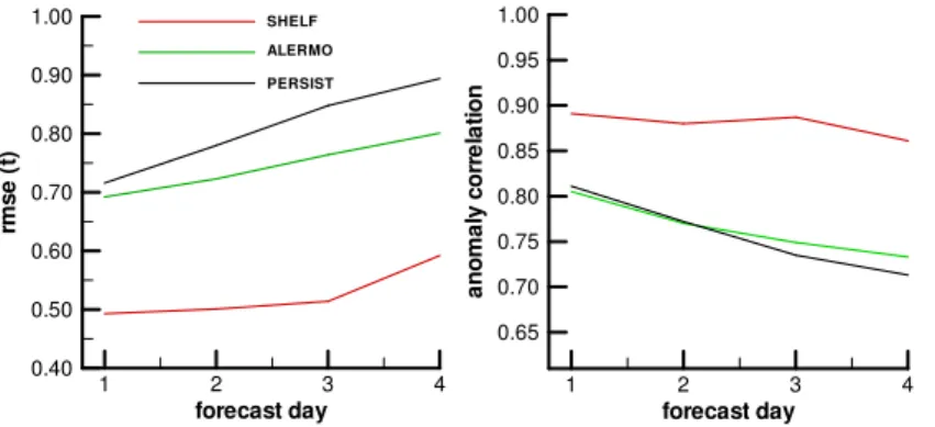
Since the satellite SST fields form the main quasi-independent verification data set available, here we will focus our attention on assessing the skill of the predicted SST fields only. In Fig. 2 we show the domain averaged RMSE (left panel) and ACC (right

20

panel) of all 48 forecasts compared to the MFSTEP analyses, as a function of fore-cast lead-time. In both panels we show the results from our shelf model as well as from the coarser resolution model, ALERMO. For comparison we also show the skill of persistence of the initial condition, which we consider to be the minimal skill reference forecast. Not surprisingly, the forecast error increases and the correlation coefficient

25

decreases with forecast lead-time indicating a reduction in skill as the forecast is longer. By both skill metrics, the shelf model is significantly superior to the coarser resolution model. Both models beat persistence, although the ACC of the coarse resolution model

(14)

OSD

3, 2059–2085, 2006

Full Screen / Esc

EGU

is not much better than persistence. Throughout the first three days of the forecasts the shelf model error remains at or below 0.5◦_{C. Throughout the forecast period, the}

ACC drops only slightly from 0.90 to 0.86, which is significantly above the commonly accepted no skill cutoff value of 0.60.

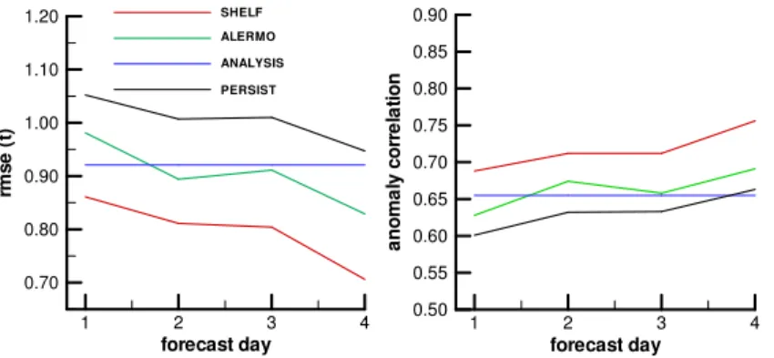
In Fig. 3 we show the SST forecast skill compared to the satellite fields. Here in

5

addition to the two models we also show the mean skill of the MFSTEP analyses for the domain of our shelf model. Contrary to expectation, here we find that forecast errors decrease and the correlation coefficients increase with forecast lead-time, thus indicating that the predicted fields are in fact improving. While we have no definitive explanation for this odd behavior, we speculate that it is related to smaller scales of

mo-10

tion that are missing in the initial conditions for the forecast, which are interpolated form the coarser resolution MFSTEP analyses. As noted above, the grid size ratio between the MFSTEP OGCM fields and the shelf model is roughly 5:1. The data assimilation system of the OGCM also has some built in filtering of the smallest resolved scales, and therefore the initial conditions are relatively smooth. As the forecast proceeds, the

15

smaller scales of motion develop in the shelf model. The satellite images also resolves these smaller scales, and therefore with time, the statistical differences between the forecast and satellite fields decrease.

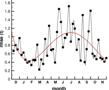
The variability of the day 1 forecast RSME compared to the satellite fields is shown in Fig. 4 for the entire study period. We have also fit a fourth degree polynomial to the

20

individual forecast points in order to highlight the seasonal behavior of the forecast skill. The errors are smallest in late winter and largest in early to mid summer. This is due in part to the seasonal variations of the surface mixed layer depth and the associated rate of change of SST. In winter when the mixed layer is deep, SST changes relatively slowly and therefore the forecast skill is highest. On the other hand in summer when

25

the mixed layer is shallow and SST variations are much larger, the model has a more difficult time producing accurate forecasts.

The spatial variability of the forecast skill is shown in Fig. 5 where we show the RMSE of the predicted SST for all 192 forecast days (48 forecasts X4 days each). The upper

(15)

OSD

3, 2059–2085, 2006

Full Screen / Esc

EGU

left panel shows the forecasts compared to the satellite fields while the upper right panel shows the forecasts compared to the MFSTEP analyses. For reference we also show the analysis error compared to the satellite fields. These maps provide further insight into the results shown in Figs. 2 and 3. In the comparison between the forecasts and the satellite fields, the errors are fairly uniform with values of 0.6–0.8◦_{C throughout}

5

most of the domain. Only along the coast do the errors increase. In the comparison between the forecasts and the MFSTEP analyses, there is a very clear tendency for the errors to decrease from the northwest, where the largest errors are about 0.8◦_C,

to values of less than 0.3◦_{C in the southeast. The comparison between the MFSTEP}

analyses and the satellite fields (lower panel) provides the explanation for this. Here we

10

see that the largest analysis errors are indeed in the northwest corner of the domain where the values exceed 1◦_{C. This relatively large analysis error is propagated to the}

model through the initial conditions, which the model clearly remembers throughout the length of the four-day forecasts. This indicates that a significant reduction in forecast error, and therefore increase in forecast skill, can be expected by improving the initial

15

conditions. One possible way to accomplish this would be to implement a local data assimilation system. The corresponding maps of ACC, which we do not show here, confirm these results.

3.2 Comparison to current meter and CTD data

While the available current meter and CTD data are rather limited, it is nevertheless

20

helpful to compare our forecasts to these data even if only qualitatively. The current meter data were available for the entire study period at a single point on the shelf in 27 m water depth off Hadera (see Fig. 1 for location). The CTD temperature and salinity profiles were available from seven stations along a cruise transect conducted on 12 Sep 2005 (see Fig. 1 for station locations).

25

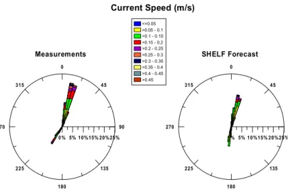
In Fig. 6 we show the current roses for the current meter measurements near Hadera and the closest model grid point for the entire study period. In terms of direction, the model does a reasonable job in terms of predicting the predominant northward, along

(16)

OSD

3, 2059–2085, 2006

Full Screen / Esc

EGU

bathymetry flow. The direction of the depth contours near Hadera is approximately 20◦

, which is consistent with the flow direction shown. While the model does a reasonable job in predicting the frequency of the currents stronger than 0.1 m/s, it tends to miss almost completely the weaker currents in the range of 0.05–0.1 m/s. During the relative infrequent period of southward flow, the currents speeds are properly predicted but the

5

directions are predicted to be mainly along the bathymetry whereas the measurements show a noticeable cross bathymetry component directed to the open sea. This may be related to the representation of the bottom drag in the model and warrants further investigation.

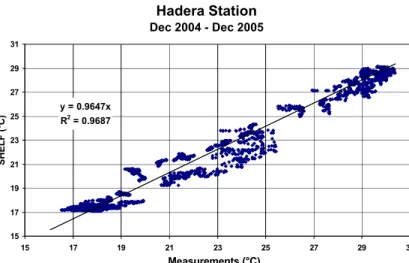
The current meter at Hadera also records temperature and in Fig. 7 we show the

10

scatter plot of the predicted versus observed temperature for the entire study period. For reference we also show the regression line as well as the correlation coefficient, which has a value of 0.97. During winter (lower temperatures), the points appear to be equally scattered above and below the line thus indicating no clear tendency in the forecast error. During the transition season and during summer there is a clear

15

tendency for the model to under predict the temperature and therefore develop a cold bias. This will also be subject to future investigation.

Finally we conclude with a comparison between the relevant forecast and the CTD temperature and salinity profiles collected during a cruise conducted on 12 Sep 2005. The locations of the seven CTD stations are shown in Fig. 1. In Fig. 8 we

summa-20

rize this comparison through a TS diagram in which we show the observed data (red points), the shelf model forecast (blue), and the coarse model forecast (green). For comparison we also include the climatological TS curve from this season taken from the MEDATLAS database. In all cases, the intermediate and deep-water masses are quite similar. The salinity maximum associate with Levantine Intermediate Water (LIW) is

25

clearly visible as is the low salinity, low temperature tail associate with Eastern Mediter-ranean Deep Water. Above the LIW layer, the observations and both models are much more saline that climatology. At sigma-t values between 26.0 and 28.5 the shelf model salinities are closer to the measured values than are the ALERMO salinities, which

(17)

OSD

3, 2059–2085, 2006

Full Screen / Esc

EGU

tend to be closer to climatology. In the topmost layer, both models under predict the very high salinity of the Levantine Surface Water (LSW), which is presumably linked to the crude specification of the surface freshwater flux in both models. We also note that the strong drop in surface salinity in the climatological curve is associated with the freshwater input from the Nile flood, which reached its annual maximum in September

5

during the pre-Aswan High Dam period, prior to 1965.

4 Summary and conclusions

In this paper we have presented the evaluation of the results from the first year of an op-erational forecasting system that was developed and implemented for the southeastern Mediterranean Sea as part of the MFSTEP project. The system is based on the

Prince-10

ton Ocean Model and is forced with lateral boundary conditions at the open boundaries taken from the regional ocean model, ALERMO run at the University of Athens, and with surface forcing taken from the atmospheric model, SKIRON, also run at the Uni-versity of Athens. ALERMO, in turn is nested in the full Mediterranean OGCM, which is run at INGV in Bologna. The respective grid sizes of the three models are 1.25, 3, and

15

6 km. Based on the assessment of 48 four-day forecasts, our conclusions regarding the forecast system are as follows:

– The model has been successfully implemented with a nesting strategy that is

stable and robust in an operational forecasting mode using high frequency forcing.

– The MFSTEP data stream, which provides the forcing fields for the forecasts, is

20

very reliable and efficient.

– For the high-resolution shelf model of the southeastern Levantine Basin, there

is clearly added value in the forecasts, which are more skillful than the coarser resolution driving models.

(18)

OSD

3, 2059–2085, 2006

Full Screen / Esc

EGU – The main limitation in forecast skill appears to be due to the analysis error, which

is inherent in the initial conditions.

As of this writing, the operational cycle of the model has already been switched to daily, rather than weekly forecasts. Since one of the main weaknesses appears to be the specification of the initial conditions, the next phase of development of the

5

system will focus on improving the methodology for specifying the initial conditions, including better interpolation and filtering of the coarse resolution fields and possibly the implementation of a local data assimilation system.

Acknowledgements. We acknowledge the support received for this work from the European Union through the Mediterranean Forecasting System Towards Environmental Prediction –

MF-10

STEP (Contract Number EVKT3-CT-2002-00075). Similarly, we thank the Ministry of National Infrastructures for their support through internal funding at IOLR.

References

Blumberg, A. F. and Mellor, G. L.: A description of a three-dimensional coastal ocean circulation model, in: Three-Dimensional Coastal Ocean Models, edited by: N. Heaps, Am. Geophys.

15

Union, Washington, DC, pp. 1–16, 1987.

Brenner, S.: High-resolution nested model simulations of the climatological circulation in the southeastern Mediterranean Sea, Annal. Geophys., 21, 267–280, 2003a.

Brenner, S.: Simulations with a relocatable, nested, high-resolution model: the eastern Levan-tine experience, in: Oceanography of the Eastern Mediterranean and Black Sea, edited by:

20

A. Yilmaz , Tubitak Publishers, Ankara, Turkey, pp. 1022–1028, 2003b.

Brenner, S., Gertman, I. and Murashkovsky, A.: Pre-operational ocean forecasting in the south-eastern Mediterranean: Model implementation, evaluation, and the selection of atmospheric forcing, J. Mar. Systems, in press, 2006.

Ezer, T. and Mellor, G. L.: Continuous assimilation of Geosat altimeter data into a

three-25

dimensional primitive equation Gulf Stream model, J. Phys. Oceanogr., 24, 832–847, 1994. Glenn, S. M., Forristall, G. Z., Cornillon, P., and Milkowski, G.: Observations of Gulf Stream

(19)

OSD

3, 2059–2085, 2006

Full Screen / Esc

EGU

ring 83-E and their interpretation using feature models, J. Geophys. Res., 95, 13 043–13 063, 1990.

Hecht, A., Pinardi, N., and Robinson, A. R.: Currents, water masses, eddies and jets in the Mediterranean Levantine Basin, J. Phys. Oceanogr., 18, 1320–1353, 1988.

Klein, B., Roether, W., Manca, B., Bregant, D., Beitzel, V., Kovacevic, V., and Luchetta, A.:

5

The large deep water transient in the eastern Mediterranean, Deep Sea Res., 46, 371–414, 1999.

Korres, G. and Lascaratos, A.: An eddy-resolving model of the Aegean and Levantine basins for the Mediterranean Forecasting System Pilot Project (MFSPP): Implementation and cli-matological runs, Annal. Geophys., 20, 205–220, 2003.

10

Korres, G., Pinardi, N., and Lascaratos, A.: The ocean response to low-frequency interannual atmospheric variability in the Mediterranean Sea, Part I: Sensitivity experiments and energy analysis, J. Climate, 13, 705–731, 2000a.

Korres, G., Pinardi, N., and Lascaratos, A.: The ocean response to low-frequency interan-nual atmospheric variability in the Mediterranean Sea, Part II: Empirical orthogonal functions

15

analysis, J. Climate, 13, 731–745, 2000b.

Lascaratos, A. and Nittis, K.: A high-resolution three-dimensional numerical study of interme-diate water formation in the Levantine Sea, J. Geophys. Res., 103, 18 497–18 511, 1998. Malanotte-Rizzoli, P., Manca, B., Ribera, M., Theocharis, A., Brenner, S., Budillon, G., and

Ozsoy, E.: The Eastern Mediterranean in the 80s and in the 90s: the big transition in the

20

intermediate and deep circulations, Dyn. Atmos. Oceans, 29, 365–395, 1999.

Manzella, G. M. R., Scoccimarro, E.,Pinardi, N., and Tonani, M.: Improved near real-time data management procedures for the Mediterranean ocean Forecasting System-Voluntary ob-serving ship program, Annal. Geophys., 21, 49–62, 2003.

Mellor, G. L.: An equation of state for numerical models of oceans and estuaries, J. Atmos.

25

Oceanic Technol., 8, 609–611, 1991.

Mellor, G. L., Ezer, T., and Oey, L. Y.: The pressure gradient conundrum of sigma coordinate ocean models, J. Atmos. Oceanic Technol., 11, 1126–1134, 1994.

Mellor, G. L. and Yamada, T.: Development of a turbulence closure scheme for geophysical fluid problems, Rev. Geophys. Space Phys., 20, 851–875, 1982.

30

MERCATOR:http://www.mercator-ocean.fr/html/mercator/index en.html, 2006. Met Office:http://www.metoffice.com/research/ncof/products.html, 2006.

(20)

OSD

3, 2059–2085, 2006

Full Screen / Esc

EGU

bo.ingv.it/mfstep, 2003.

MFSTEP: Monthly Bulletin,http://www.bo.ingv.it/mfstep/WP8/monthly.htm, 2006.

Orlanski, I.: A simple boundary condition for unbounded hyperbolic flows, J. Comput. Phys., 21, 251–269, 1976.

Pinardi, N., Allen, I., and Demirov, E.: The Mediterranean Ocean Forecasting System: the first

5

phase of implementation, Annal. Geophys., 21, 3–20, 2003.

POEM Group: The general circulation of the Eastern Mediterranean. Earth-Sci. Rev., 32, 285– 309, 1992.

Robinson, A. R., Hecht, A., Pinardi, N., Bishop, J., Leslie, W., Rosentroub, Z., Mariano, A. J., and Brenner, S.: Small synoptic/mesoscale eddies and the energetic variability of the

10

eastern Levantine basin, Nature, 327, 131–134, 1987.

Robinson, A. R., Haley, P. J., Jr., Lermusiaux, P. F. J., and Leslie, W. G.: Predictive skill, predic-tive capability and predictability in ocean forecasting, in: Oceans02, MTS/IEEE Publication, Mar. Technol. Soc., Columbia, MD, pp. 1234–1241, 2002.

Rosentraub, Z. and Brenner, S.: Circulation over the southeastern continental shelf and slope of

15

the Mediterranean Sea: Direct current measurements, winds, and comparison to numerical simulations, J. Geophys. Res., under revision, 2006.

Roussenov, V., Stanev, E., Artale, V., and Pinardi, N. : A seasonal model of the Mediterranean Sea general circulation, J. Geophys. Res., 100, 13 515–13 538, 1995.

Rowley, C., Barron, C., Smedstad, I., and Rhodes, R.: Real-time ocean data assimilation and

20

prediction with global NCOM, in: Oceans02, MTS/IEEE Publication, Mar. Technol. Soc., Columbia, MD, pp. 775–780, 2002.

Wu, P. and Haines, W.: The general circulation of the Mediterranean Sea from a 100-year simulation, J. Geophys. Res., 103, 1121–1135, 1998.

Wu, P., Haines, K., and Pinardi, N.: Toward an understanding of deep-water renewal in the

25

Eastern Mediterranean, J. Phys. Oceanogr., 30, 443–458, 2000.

Zavatarelli, M. and Mellor, G. L.: A numerical study of the Mediterranean Sea circulation, J. Phys. Oceanogr., 25, 1384–1414, 1995.

(21)

OSD

3, 2059–2085, 2006

Full Screen / Esc

Printer-friendly Version Interactive Discussion EGU 20 0 20 0 200 40 0 40 0 400 60 0 60 0 80₀ 80 0 800 10 00 10 00 1200 12 00 12 00 14 00 14 00 1600 160 0 1800 33.5 34 34.5 35 31.5 32 32.5 33 33.5 HAIFA HADERA

Fig. 1. Domain, bathymetry and portion of grid for the southeastern Levantine narrow shelf

model. The dots show the locations of in situ verification data, which were available from a current meter station near Hadera and from a series of hydrographic stations along a section extending seaward Haifa as explained in Sect. 3.

(22)

OSD

3, 2059–2085, 2006

Full Screen / Esc

Printer-friendly Version Interactive Discussion EGU forecast day rm s e (t ) 1 2 3 4 0.40 0.50 0.60 0.70 0.80 0.90 1.00 SHELF ALERMO PERSIST forecast day a n o m a ly c o rr e la ti o n 1 2 3 4 0.65 0.70 0.75 0.80 0.85 0.90 0.95 1.00

Fig. 2. Forecast skill compared to daily MFSTEP analyses for all forecasts as a function of

forecast lead-time, for the shelf model, ALERMO, and persistence: Root mean square error (left panel) and anomaly correlation coefficient (right panel).

(23)

OSD

3, 2059–2085, 2006

Full Screen / Esc

Printer-friendly Version Interactive Discussion EGU forecast day rm s e (t ) 1 2 3 4 0.70 0.80 0.90 1.00 1.10 1.20 SHELF ALERMO PERSIST ANALYSIS forecast day a n o m a ly c o rr e la ti o n 1 2 3 4 0.50 0.55 0.60 0.65 0.70 0.75 0.80 0.85 0.90

Fig. 3. Forecast skill compared to daily satellite analyses for all forecasts as a function of

forecast lead-time, for the shelf model, ALERMO, and the MFSTEP analyses: Root mean square error (left panel) and anomaly correlation coefficient (right panel).

(24)

OSD

3, 2059–2085, 2006

Full Screen / Esc

Printer-friendly Version Interactive Discussion EGU month rm s e (t ) 0 0.2 0.4 0.6 0.8 1 1.2 1.4 1.6 1.8 D J F M A M J J A S O N

Fig. 4. Temporal variability of the day 1 forecast root mean square error for all forecasts in the

(25)

OSD

3, 2059–2085, 2006

Full Screen / Esc

Printer-friendly Version Interactive Discussion EGU 33.5 34 34.5 35 31.5 32 32.5 33 33.5 1.25 1.1 0.95 0.8 0.65 0.5 0.35 0.2 0.05 RMSE (fcst-anl) 33.5 34 34.5 35 31.5 32 32.5 33 33.5 RMSE (fcst-sat) 33.5 34 34.5 35 31.5 32 32.5 33 33.5 RMSE (anl-sat)

Fig. 5. Spatial variability of the root mean square error for all 192 forecast days in the study

pe-riod: Forecast compared to satellite analyses (upper left panel), forecast compared to MFSTEP analyses (upper right panel), and MFSTEP compared to satellite (lower panel).

(26)

OSD

3, 2059–2085, 2006

Full Screen / Esc

Printer-friendly Version Interactive Discussion EGU 0 45 90 135 180 225 270 315 0 % 5% 10%15% 20%25% <=0.05 >0.05 - 0.1 >0.1 - 0.15 >0.15 - 0.2 >0.2 - 0.25 >0.25 - 0.3 >0.3 - 0.35 >0.35 - 0.4 >0.4 - 0.45 >0.45 Measurements 0 45 135 180 225 270 315 0 % 5% 10%15% 20%25% SHELF Forecast Current Speed (m/s)

Fig. 6. Current roses at Hadera for the observed (left) and predicted (right) currents for all

(27)

OSD

3, 2059–2085, 2006

Full Screen / Esc

Printer-friendly Version Interactive Discussion EGU Hadera Station Dec 2004 - Dec 2005 y = 0.9647x R2 = 0.9687 15 17 19 21 23 25 27 29 31 15 17 19 21 23 25 27 29 31 Measurements (°C) SH EL F (° C )

Fig. 7. Scatter plot of observed and predicted temperatures at Hadera for all forecast days in

(28)

OSD

3, 2059–2085, 2006

Full Screen / Esc

EGU Haifa Section 12, September 2005

Most West Long.=33.70, Most East Long.=34.92, Most South Lat. =32.90, Most North Lat. =33.00

38.5 38.6 38.7 38.8 38.9 39 39.1 39.2 39.3 39.4 39.5 Salinity (psu) 12 14 16 18 20 22 24 26 28 T e m p ( C ) - Climate - ALERMO - SHELF - Measured Data

Fig. 8. TS diagram along a cruise transect from 12 Sep 2005 showing the observed and

predicted values from the shelf model and from ALERMO. The climatological TS curve is shown for reference.