Application of Bicoherence Analysis in Study of Wave Interactions in Space Plasma

HAL Id: insu-02880211

https://hal-insu.archives-ouvertes.fr/insu-02880211

Submitted on 24 Jun 2020

HAL is a multi-disciplinary open access

archive for the deposit and dissemination of

sci-entific research documents, whether they are

pub-lished or not. The documents may come from

teaching and research institutions in France or

abroad, or from public or private research centers.

L’archive ouverte pluridisciplinaire HAL, est

destinée au dépôt et à la diffusion de documents

scientifiques de niveau recherche, publiés ou non,

émanant des établissements d’enseignement et de

recherche français ou étrangers, des laboratoires

publics ou privés.

Application of Bicoherence Analysis in Study of Wave

Interactions in Space Plasma

Dominique Lagoutte, François Lefeuvre, J. Hanasz

To cite this version:

Dominique Lagoutte, François Lefeuvre, J. Hanasz. Application of Bicoherence Analysis in Study

of Wave Interactions in Space Plasma. Journal of Geophysical Research Space Physics, American

Geophysical Union/Wiley, 1989, 94 (A1), pp.435-442. �10.1029/JA094iA01p00435�. �insu-02880211�

JOURNAL OF GEOPHYSICAL RESEARCH, VOL. 94, NO. A1, PAGES 435-442, JAUUARY 1, 1989

Application of Bicoherence Analysis in Study of

Wave Interactions in Space Plasma

D. LAGOUTTE and F. LEFEUVRE

Laboratoire de Physique et Chimie de l'Environnement, CNRS, Orldans, France

J. HANASZ

Copernicus Astronomical Center, Torun, Poland

A spectral analysis at the second order (power spectrum) loses the phase information among the different Fourier components. To retain this information, the bispectrum (third order) and/or the bicoherence (normalized bispectrum) are calculated. Application to simulated data, shows the dependence of the bispectrum to amplitudes of involved waves and of the bicoherence to signal-to-noise ratio. Bicoherence technique is applied in the analysis of harmonics produced by an electronic receiver, as well as in the investigation of phase coherence between a ground-transmitter signal, a natural ELF emission near the proton gyrofrequency, and the sidebands around the carrier. Strong arguments are provided that

the sidebands are generated by a parametric interaction between the transmitter signal and the ELF emission.

1. INTRODUCTION

Several suggestions of possible wave-wave interactions in

the ionosphere and the magnetosphere have been reported. For example, Riggin and Kelley [1982] have suggested that

parametric decay of whistler mode waves into lower hybrid

waves may occur for strong natural or artificial emissions.

Koons et al. [1987] have observed the generation of ion

acoustic waves from the decay of Langmuir waves near the electron plasma frequency. Wave-wave interactions have been proposed to explain the auroral kilometric radiation, specifically the narrow bands [e.g., Roux and Pellat, 1979;

Grabbe et al., 1980; Altman et al., 1987], although on the

other hand the maser process has been admitted for several years as being responsible for this radiation [Wu and Lee,

1979]. A bicoherence analysis of the waveform observed with

ARCAD 3, supports the suggestion that a nonlinear-mode

coupling between the transmitter pulse and ELF emission can

produce the sidebands around the transmission frequency [Tanaka et al., 1987].

The use of bicoherence technique has also appeared to be very successful in studies of wave phenomena in various media, such as harmonic generation of ocean-surface gravity waves [Elgar and Guza, 1985], brain wave emissions [Huber

et al., 1971 ], nonlinear transfer of energy in turbulent flows [Lii et al., 1976; Van Atta, 1979], and nonlinear interaction

between modes of density fluctuations in laboratory plasmas

[Kim and Powers, 1979; Kim et al., 1980]. Furthermore, the

considerable amount of literature regarding higher-order spectral analysis is so well known that it barely needs

mention here.

The higher-order spectral analysis appears to be unique in attempts to answer the question of the presence of multiwave

interaction processes, because phase information is not lost in it. This is why, in the era of fast analog-to-digital converters

and large random-access memories, the method of bicohe- rence analysis is expected to be increasingly used in studies

of wave generation in space plasmas.

Numerous difficulties exist with the application of the bicoherence technique to space experiments. First, full waveforms, sometimes in very large bands, must be teleme-

Copyright 1989 by the American Geophysical Union.

Paper number 7A9462.

0148- 0227/89/007A- 9462505.00

tered to the ground, a condiiion

that is generally incompati-

interaction to take place (f3 = fl + fu,, K3 = K 1 + Ku,) is

expected to be satisfied in the source region only. Third, the bicoherence analysis only allows the detection of quadratic nonlinear interactions, whereas a higher order of interactions may be produced in space plasmas. The present study shows that, despite all those difficulties, the bicoherence technique does detect three- wave nonlinear interactions in space.

The aims of this paper are to describe the bicoherence analysis as applied to the wave data collected in space experiments, to illustrate how the method can be applied to the specific data obtained in the wave experiment of ARCAD 3, and to show the advantages and limits of the

method.

The plan of the paper is as follows. First, the basic definitions of the bispectrum and bicoherence are recalled (section 2). Then, simulated data are analyzed to show how estimators of the bispectrum and bicoherence can describe the phase coherence of the interacting signals, and to highlight the problems that arise when one or the other is used (section 3). Section 4 is devoted to the analysis of experimental data recorded on ARCAD 3, characteristic for the sidebands accompanying the VLF transmission in the presence of ELF emission. Conclusions are presented in section 5.

2. DEFINITIONS AND PROPERTIES

2.1. Basic Definitions

Let x(t) be a real and stationary signal with zero mean

value and X(f) its Fourier transform.

Hereafter, X k, the

Fourier component

at the frequency

fk is noted as

T

X k = .[ x(t) exp

(- 2•rJfkt)

dt

(1)

The definitions of the second moment of the time series

concern autocorrelation and the power spectrum. The autocorrelation for the record (i) at the time lag r is defined by

1 [T x(i)(t

) x(i)(t

+ r) dt

(2)

R

(i)

(r)

--• o'

z136

Lagoutte et al' Bicoherence Analysis and Wave Interactions

The po•ver spectrum

at the frequency

fk is the Fourier

I

,,

T i

S(k)

-- S(f

k) -- Tf R(r)

exp(-

2•rjf

k r) dr

(3)

':

where

R(r)-- E{R(i) (r)}.

An alternate equivalent way is [Bendat and Piersol, 1971]

where the average E { } is taken over i -- 1 .... M successive

data

records,

and

X•c

is the

complex

conjugate

of X k.

Similarly, the third moment

at the time lags r• and r9. is

R(r•,

rp.)

--

E{•

lrx(i)(t)

x(i)(t•-r•)

. x(i)(t•-rp.)

dt)

(5)

and, by definition, the bispectrum

at the frequencies

fk and

fl is the two-dimensional

Fourier transform

of R(r•, r9.):

-T -T

ß

exp(- 2•rj (fkr• •- flr•.)) dr• dry. (6)

Now, the bispectrum can be defined as a product of three Fourier components [Kim and Powers, 1979]:

B(k,

l) = lira 1 E{•) X(•)

_{T-•oo •}

xCi)"• (7)

_k•-lJ

But this definition is only valid if the sum of the frequencies of the three Fourier components is zero, which means

fk4-1--

fk 4-_

fl

(8)

where

fk•-I is the frequency

of the product

wave in case

of

coupling. The bicoherence spectrum is a normalized

bispectrum:

b9'(k,1)

__

(9)

E{I

XkX11•')

E([Xk4.1

[u')

The variance of b(k,l) is expressed as

_• 1 [1 - b

2(k,l)•

(10)

var

•b(k,1)• •r

For more details about the above definitions, see Kim and Powers [ 1979].

The bispectrum and bicoherence are important tools to investigate the phase coherence between three Fourier

components

of frequencies

fk, fl, fk•-l. If the third wave at

the frequency fk•-I -- fk •' fl is spontaneously

emitted, the

phase

of the Fourier component

Xk•. l will be independent

of

the phase

of the two others,

X k and X 1, and the values

of

bispectrum (7) and bicoherence (10) will be zero. On the

other hand, if the wave at the frequency fk+l is phase

and bicoherence will be nonzero. 2.2. Computation Region

The frequencies

fk, fl and fk,l are limited by the

maximum frequency fN of the studied signal. The total

B(k,l)

= B(I,

k)-- B*(-k,

-l)-- B*(-k,

k4-l)

(1

1)

(a) (b)

(c)

Fig. 1. Region of computation of bispectrum and bicohe- rence spectrum. (a) Hexagonal area (dashed line) is the

definition region. Due to symmetry relations, the bispectrum is calculated over the triangle A, and the bicoherence over

the triangle A for sum interaction (k, l -• k •- /), and over

the triangles B1, B2 for difference interaction (k,-l -• k - l). (b) Coordinate transformation for the region of computa- tion of bicoherence spectrum for difference interaction. (c) Restricted area of computation (hatched rectangle)in case of memory limitation.

one can limit the computation of the bispectrum on the A region, which is the triangle defined by

O< fl• fN/2 fl < fk < fN- fl

This is somewhat different for the bicoherence. Due to the

normalization in the bicoherence definition (9), a symmetry has been lost and we only have

b(k, l) -- b(1, k) = b(-k, -1) (12) Then, the restricted region for the bicoherence computation is formed by the A, B1 and B2 areas in Figure la. The A region is for the sum interaction k,l--} k•-l, and the (BI+B2) region is for the difference interaction k,-l--} k-l. (B1 : k, -l-• k-l with k-l >_ l, and B2: k, -l--} k-lwith k-l<l) with an appropriate change of variables, whereas the B 1 and B2 regions can be represented like the A region (Figure lb). The shape of the three areas is now the same, but with

different variables on the axes.

When high-frequency resolution is needed, the problem of computer memory arises, because the area of the triangle is

N/2 . N/4 • N9'/8, where N is the number of samples in a

record. The way to overcome this problem, is to select a restricted area of computations as shown by the hatched rectangle in Figure lc.

3. APPLICATION TO SIMULATED DATA

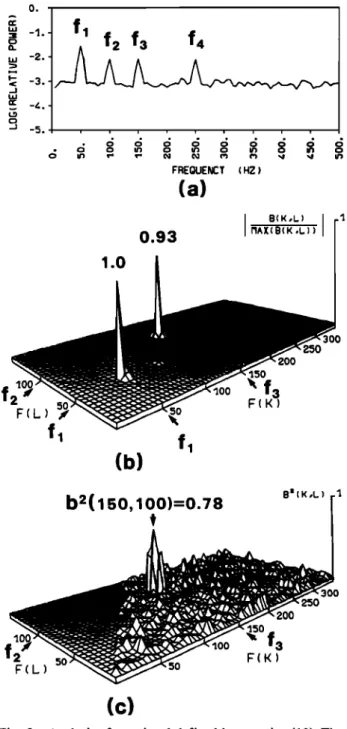
A test signal is considered in such a manner that

x(t) = 2cos(2•rf

xt4-•b•)

4-cos(2•rf•.t44bu.)

4-cos(2•rfst4-•bs)

4-cos(2•rf4t4-•b4)

4- N(t)

(13)

with fz = 50 Hz, f•. = 100 Hz, fs = 150 Hz, f4 = 250 Hz and

a sampling frequency of 2000 Hz. The phases Oz, •9., Os are

randomly

distributed

over [-•r• + •rJ and the phase

•P4

= •P•.

+ •Ps.

N(t) is a white gaussian

noiseß

With the phase coherence for the waves at frequencies f•.,

rs, /'4, we expect a nonzero value for the bispectrum

and

bicoherence

at these frequencies

(B(f s, f•.) and b(/' s, f•.)) and

a zero value otherwiseß

The autospectrum of the signal x(t) is shown in Figure 2a, and the bispectrum and bicoherence spectrum in Figures 2b and 2c. The bispectrum has two peaks, whereas only one was

expected. The peak at frequencies f•. and fs is correct,

Lagoutte et al' Bicoherence Analysis and Wave Interactions t•37 0o

I

f

f

•

f2 3

4

• -2.

• -:3.

(a)

I 8(K,L)

(b)

fl

b2(150,100)=0.78

xf 3

'"•'

,•oo f3

f2

F(K)

(c)

Fig. 2. Analysis of test signal defined by equation (13). The

FFT is performed with N = 400 samples in each record, and the average is taken over M= 30 data records. Frequency resolution is 5 Hz. (a) Autospectrum. (b) Bispectrum. (c) Bicoherence spectrum.

/z'/s and their sum/4 =/•. +/s-However, the peak B(/l, fl)

has no physical meaning. Though /•. = /x + /x, there is no

this second peak is that the bispectrum is very sensitive to the

amplitudes of the involved spectral components. This example

shows clearly that, even for incoherent signals, the value of

the bispectrum can be significant, if the averaging is performed on too small a number of records (in this case M =

30). The conclusion must be that the use of the bispectral estimator can be misleading; for this reason, the following

analysis will deal only with the bicoherence analysis.

In Figure 2c, only the expected

peak b•'(/s

,/•.) is present.

Although the waves at frequencies /•., /s, /4 = /•. +/s are

phase coherent, the maximum value of the bicoherence

estimator

is only b•'(fs, f•.) -- 0.78 instead

of 1. This is due to

the noise N(t), added to the test signal. Although, theoreti-

cally, the bispectrum is independent of noise [Lagoutte, 1953], the bicoherence is very sensitive to S/N due to the

normalization. If this ratio is low, the value of bicoherence estimated with a relatively small number of data records (M < 50) can be non significant, even in the case of phase coherence. To recover significant value the number of data records must be increased (up to several hundred) at least if the signal is stationary over a sufficiently long time interval.

Another problem in experimental applications of bicohe- fence technique is how to digitize the signal, eight-bit samples being commonly used. Our simulations show that, even with three-bit sampling, the bicoherence spectrum is practically identical to the one obtained with the eight-bit sampling, whereas with two-bit sampling spurious peaks appear in the bicoherence spectrum.

In conclusion to this section, it can be said that the use of bispectrum analysis can be subject to wrong interpretation. Bicoherence can only be used if the waves are not embedded in noise. Digitization of a signal to three-bit or larger samples will not distort the bicoherence spectra.

4. APPLICATION TO ARCAD 3 DATA

The data were recorded on board the AUREOL 3 satellite,

which formed part of the Soviet-French project ARCAD 3

for the study of the ionosphere and magnetosphere. In this

case, the working mode C2 of the VLF experiment

[Berthelier et al., 1982] was of interest. In this mode, one

electric or one magnetic component in a 70-Hz to 16-kHz bandwidth was telemetered during a 4-s time interval. On a

spectrogram (not shown in this paper) of the E H component

(E H is in a plane 11 ø off the plane perpendicular

to B o)

coordinates 50.5øN, 137øE). The three different frequencies

are 11.9 kHz, 12.65 kHz, and 14.9 kHz, and each pulse has a duration of 400 ms. A spectral broadening of the carrier

frequency was also observed. According to Tanaka et al. [1987], this phenomenon can be described in two types: (1)

without sideband structure; (2) with sideband structure,

observed only on the E H component.

The power spectra

presented in Figures 4a and 5a, clearly show the sideband

structure around the carrier frequency (respectively 11.9

kHz and 12.65 kHz) and also a strong ELF emission at and

above 500 Hz. In section 4.2, the phase coherence among

these different waves will be investigated by means of the bicoherence estimator.

When analyzing ARCAD 3 data, interference is commonly encountered, which is generated by the spacecraft system and

shows harmonic structures. Here, bicoherence analysis will be used to answer the question whether these structures are phase coherent.

4.1 Analysis of Harmonics

Figure 3a represents an autospectrum of the E H component

from 0 up to 15 kHz. The VLF-transmitter signal at 11.9

kHz and a number of harmonics of • 800 Hz can be

seen, and Figure 3b shows the map of their bico-

herence spectrum. One can conclude from it the following:

1. Harmonics are phase coherent with a maxi-

mum value of the bicoherence b•-(2.4, 1.6)= 0.92,

which indicates that some nonlinear process must be operating at the fundamental frequency of • $00 Hz.

2. The horizontal, vertical and 45 ø structures of weak peaks in the bicoherence spectrum can be easily explained if

•438

Lagoutte et al.' Bicoherence Analysis and Wave Interactions

EH

• , •

Transmitter

(b)

Fig. 3. Spectral and bicoherence analyses of the electric E H

component recorded on September 29, 1982, at 2225:6.5 UT.

Analyses are performed with N = 500 samples in each record

and the average is taken over M = 38 data records. Frequency resolution is 100 Hz. (a)Autospectrum. Arrows indicate harmonics of • 800 Hz. (b)Bicoherence spectrum.

one takes into account that fourth, eigth, twelth, etc., peaks in the power spectrum are of low magnitude. As the

bicoherence estimator is very sensitive to S/N, its correspon-

ding values

along

lines where fk, fl, fk+l are multiples

of the

fourth harmonic, will be weaker than the ones at points corresponding to other harmonics.

4.2. Analysis of Spectral Broadening of the Transmitter Signal

Five cases of spectral broadening, characteristic for sidebands around the carrier at, E H component have been already analyzed [Tanaka et al., 1987]. For the purpose of

this paper, only two cases were selected, which appeared to be the best for illustrating how the bicoherence analysis

works.

4.2.1. Transmitter frequency 11.9 kHz, time 0423:11.4. The power spectrum presented in Figure 4a shows the two distinct sidebands, the lower being at 11.4 kHz and the

upper at 12.4 kHz. Within the low-frequency range, a peak

of ELF emission is observed at 500 Hz. Since these types of

waves satisfy the frequency condition for parametric interaction, a coupling between transmitter and ELF waves is expected, which produces the sideband emissions. Therefore the region of interest is limited to the rectangle of frequency

intervals : 9.5 to 15 kHz and 0 to 3 kHz. As explained in

section 2, the studies of sum interaction and difference

interaction are done on two different plots. The bicoherence

spectrum for the sum interaction (upper sideband) is displayed in Figures4b and 4c, and for the difference

(lower sideband) in Figures 4d and 4e. The main peak, b 2

(11.9, 0.5) -- 0.65, shows a phase coherence between the transmitter (11.9 kHz), the ELF emission (0.5 kHz) and the upper sideband (12.4 kHz). The value of the bicoherence is significant, though S/N in the power spectrum is low at sideband frequencies. The bicoherence estimator for the

lower sideband is b •- (11.9, - 0.5) -- 0.53. Again, even though

the bicoherence value is lower than previously, it can be concluded that the transmitter signal, ELF emission and lower sideband are phase coherent. The interpretation of peaks of minor bicoherence value (secondary peaks) will be given in the following subsection.

4.2.2. Transmitter frequency 12.65 kHz, time 0423:28.8. The power spectrum is presented in Figure 5a, bicoherence results for sum interactions (upper sideband) in Figures 5b and 5c, and for difference interaction (lower sideband)in

Figures 5d and 5e. The maximum

values are b 2 (12.7, 0.5) --

0.65 and b • (12.6, -0.5) -- 0.68, which means that here again phase coherence exists for all three types of waves.

In all the bicoherence maps secondary peaks can be

identified. For instance, in Figure 5c, for sum interaction,

three secondary

peaks

exist at fk-- 11.7, 12.2, and 13.2 kHz

and the main peak at 12.7 kHz, the latter having been

discussed

in the preceding

subsection.

The peak b • (12.2, 0.5)

emission and transmitter. Physically, the product wave of

interaction is the lower sideband and thus the correct

denominator in the normalization (formula(9)) is E{I

2

2},

Xo.s I } . E{IX•.•

I

which has been used for the

corresponding peak in Figure 5e. To obtain the result in

Figure 5c, looking

for sum

interaction,

one normalizes

with

the

denominator

E( I X•2.s

Xo.

s I-) ß E( I X•s.7

IS),

which

is

incorrect because the carrier is not a product wave.

Now the two other secondary peaks of bicoherence

spectrum

at fk -- 11.7 and 13.2 kHz (Figure 5c) should

be

considered. At these frequencies, faint sidebands can be identified in the power spectrum (Figure 5a), which will be

called the secondary sidebands. These bands are phase coherent with the primary sidebands and ELF emission,

which can be concluded from the bicoherence spectrum

(f k+•l = f k+l + f l, f k-2l = f k-I - f l)' Though

one can expect

phase coherence between the carrier and the secondary sidebands, the bicoherence analysis is not able to prove it directly, because the frequency condition (equation (8)) is not satisfied.

4.2.3. Discussion. Two of the five cases of the sideband

emissions, which appear in the power spectrum in the presence of transmitter emission and ELF noise, have been presented in this paper to illustrate the application of the bicoherence technique to wave experiments in space.

According to Tanaka et al. [1987], the sidebands can be

interpreted in terms of the three-wave interactions of plasma waves, whereas the electronic receiver is suggested to be

excluded as a source of a nonlinear process between the

transmitter and ELF signals.

The use of the momentum conservation law (K k :• K l =

Kk+l) could confirm Tanaka's et al.'s interpretation.

measured at a given time. It can, however, be expected that in this type of parametric process the energy of the secondary

waves observed at sideband frequencies is produced at the

expense of the primary waves of the carrier and ELF

emission. But, due to the lack of knowledge about the transfer function of the receiving equipment, it was not possible to verify quantitatively the power-density balance

for the suggested process. Nevertheless, a strong confirma-

tion was obtained that the sidebands have a natural origin and are produced in the parametric process. In Figures 6a

and 6b, time dependencies are presented for the powers received at the frequencies of interacting waves with the transmitter frequency at 11.9 and 12.65 kHz, respectively.

Lagoutte

et al' Bicoherence

Analysis

and Wave Interactions

439

EH

fk

(a)

F (L:) •. •o'

•,,•

,o.•o

l 1.9

:.z•

0.5

• .

(b)

0.5

'•o.5

'

(c)

(d)

'•o.5

' !.•.•.5

'

ll.4 (e)

Fig. 4. Spectral

and

bicoherence

analyses

of the E H component

recorded

on August

11, 1982,

at 0423:11.4

UT. The satellite

coordinates

are altitude 1178 kin, geographic

latitude

46ø7, geographic

longitude

135ø5.

Analyses

are performed

with N = 500 samples

in each

record

and the average

is taken

over

M = 38 data

records.

Frequency

resolution

is 100 Hz. (a) Autospectrum.

The frequencies

fk' fl' fk+l' fk-I represent,

respectively,

the frequencies

of the transmitter

signal

(11.9 kHz), the ELF emission,

and

the upper

and

the

lower sidebands.

(b) Three-dimensional

plot of the bicoherence

spectrum

for sum interaction

(upper

sideband).

(c) Same

as (b) with contour

levels.

(d) Three-dimensional

plot of bicoherence

spectrum

for

difference interaction

(lower sideband).

(e) Same

as (d) with contour

levels.

Each point represents the power value at the relevant

frequency, estimated

from the Fourier transformation

of $00

samples.

The powers are expressed

in arbitrary units and

cannot be comparedß It can be seen that the power of the sidebands is increased when the ELF emission is strong and

when the transmitter emission is simultaneously decreased.

This observation shows qualitatively that the parametric

process is operating only when ELF emission is strong

enough, and the power in the sidebands

can be generated

at

the expense of the transmitter power. Due to the lack of

calibrated data, it was not possible to measure the coupling coefficient for this process, the parameter essential in understanding the energy transfer for the three-wave

qq0

Lagoutte et al' Bicoherence

Analysis

and Wave Interactions

(a)

b2 (12.7,0.5)•0.65

2.TF(K)

0.5 c;

. (• • {]

0.5

.•o

9.s

•o.s

'/•.s

•2.5

•'3

(b)

(c)

12.?

b•(• •_.6,-o.•)=o.68

,•-.

so

• ,-:

.

F1•.5o

.T'

.•

0• 0•

)

F ( L ) l"tø

•o.

so

( KHZ

)

"

<

•<HZ

)

0.5

12.1

d , , - ...

(d)

(e)

Fig. 5. Same

as Figure 4 at 0423:28.8

UT and transmitter

frequency

12.65 kHz. The satellite

coordinates

are altitude 1191 km, geographic

latitude 45ø7, geographic

longitude

135ø7.

One has also to be careful with applying the bicoherence

analysis in case of slow electrostatic waves received on a

moving spacecraft, as their Doppler shift frequencies can no longer satisfy the frequency condition (8). The effect can be

insignificant

when the bandwidth

of spectral

analysis

or the

natural bandwidths of the involved waves are larger than the

frequency shift (which is the case here). However, it has

been proved by Lagoutte [1983] that even for Doppler-

shifted frequencies

the bicoherence

values

do not change

if

the spacecraft is in the source region, i.e., when the wave

number condition is still satisfied.

5. CONCLUSION

The application of bicoherence analysis to the geophysical data collected in the wave experiment on ARCAD 3 is demonstrated by using two of the five cases of wave interactions at frequencies of the transmitter, ELF emission and the sidebands, as suggested already by Tanaka et al.

[1987]. The conclusions

from the present study are as

follows:

1. The analysis of bicoherence spectra is successful for establishing the phase coherence in the received data at

Lagoutte et al' Bicoherence Analysis and Wave Interactions 60. 55- I,l,,I 45- • 40- 35- 30- I 1/08/1982 04.23.11.400

ß • Transmitter

(11.9

khz)

I • I I

•ELF

emission

• [ • t

3

1oo

;so

I

• •e• .e- -e•

•

?

:

, ,'

,

_,

Fig. 6. Time dependence of powers at the frequencies of the interacting waves. One value of power is obtained by a spectral analysis with N = 500 samples, which corresponds to 10-rns data. The corresponding symbols are circles for the transmitter, triangles for the ELF emission, and squares for the averaged power of the lower and upper sidebands. The hatched area represents the loss of power of the transmitter. (a) transmitter frequency 11.9 kHz, time 0423:11.4 UT. (b) transmitter frequency 12.65 kHz, time 0423:28.8 UT.

frequencies of the suggested interaction process. However, to

demonstrate its operation in space plasma, information on wave vectors and transfer functions of the receiving equipment is required as well.

2. New and strong confirmation is provided for the

parametric interactions of the investigated waves; increased sideband power is observed when ELF emission is high and the transmitter signal is decreased simultaneously.

3. The application of the method faces some limitations, such as the following ß (1) The bicoherence estimator depends on the signal-to-noise ratio in such a way that, with decreasing S/N, the bicoherence value decreases to zero, even if the coupling in the wave interaction is high. If the signal is stationary over a sufficiently long time interval, one can recover a nonzero value by averaging over a large number of data records. (2) The digitizing of the analog signal has to be done with samples of at least three-bit length, as two-bit

sampling produces spurious peaks in the bicoherence spectrum. (3) By definition, the bicoherence analysis is limited to the case of the three-wave interaction (quadratic)

only.

4. It is shown that the interpretation of the bispectrum estimator can be misleading, since even for incoherent signals

the value of the bispectrum can be significant for large

spectral-component amplitudes and a limited number of records (M).

5. While interpreting the bicoherence spectra, one has to be careful about defining interacting waves and a product wave.

The confusion of these two in the normalizing denominator

leads to an incorrect value of bicoherence.

6. No knowledge is required about a transfer function of a

receiver at frequencies of interacting waves, for the

estimation of bicoherence; however, this is essential for

determinations of the coupling coefficient, bispectrum phase

and energy balance in a process of three-wave interaction. Acknowledgments. We acknowledge J. J. Berthelier as principal investigator and instigator of the ARCAD 3 VLF

experiment. We also thank CNES (Toulouse), especially D.

Fournier, for the data processing and we are grateful to J. J. Blecki, P. Oberc, and J. Majewski, who first turned our

attention to the use of bicoherence in the study of waves in

the magnetosphere.

The Editor thanks R. A. Helliwell and another referee for

their assistance in evaluating this paper.

REFERENCES

Altman C., B. Lamb•ge, and A. Roux, Generation of non-thermal E.M. continuum, paper presented at 22nd General Assembly, URSI, Tel Aviv, 1987.

Bendat, J. S., and A. G. Piersol, Random Data: Analysis and Measurement Procedures, John Wiley, New York, 1971. Berthelier, J. J., F. Lefeuvre, M. M. Mogilevsky, O. A.

Molchanov, Yu. I. Galperin, J. F. Karczewski, R. Ney, G.

Gogly, C. Guerin, M. L6v•que, J. M. Moreau, and F. X.

Sen6, Measurements of the VLF electric and magnetic components of waves and DC electric field on board the AUREOL-3 satellite: The TBF- ONCH experiment, Ann.

Geophys., 38, 643, 1982.

Elgar, S., and R. T. Guza, Observations of bispectra of shoaling surface gravity waves, J. Fluid Mech., 169, 425,

1985.

Grabbe, C. L., K. Papadopoulos, and P. J. Palmadesso, A coherent nonlinear theory of auroral kilometric radiation,

1, Steady state model, J. Geophys. Res., 85, 3337, 1980. Huber, P. J., B. Kleiner, T. Gasser, and G. Dumermuth,

Statistical methods for investigating phase relations in stationary stochastic processes, IEEE Trans. Audio

Electroacoust., 19, 78, 1971.

Kim, Y. C., and E. J. Powers, Digital bispectral analysis and

its applications to nonlinear wave interactions, IEEE

Kim, Y. C., J. M. Beall, and E. J. Powers, Bispectrum and nonlinear wave coupling, Phys. Fluids, 23, 258, 1980. Koons, H. C., J. L. Roeder, O. H. Bauer, G. Haerendel, R.

14•42 Lagoutte et al.: Bicoherence Analysis and Wave Interactions

Treumann, R. R. Anderson, D. A. Gurnett, and R. H. Holzworth, Observation of nonlinear wave decay processes

in the solar wind by the AMPTE IRM plasma wave experiment, J. Geophys. Res., 92, 5865, 1987.

Lagoutte, D., Analyses spectrale et bispectrale de champs

d'ondes 61ectromagnStiques: Mod81e AR vectoriel et bicoherence, th•se 3•me cycle, Univ. d'OrlSans, OrlSans, France, 1983.

Lii, K. S., M. Rosenblatt, and C. Van Atta, Bispectral mbasurements in turbulence, J. Fluid Mech., 77, 45, 1976.

Riggin, D., and M. C. Kelley, The possible production of

lower hybrid parametric instabilities by VLF ground transmitters and by natural emissions, J. Geophys. Res., 87, 2545, 1982.

Roux, A., and R. Pellat, Coherent generation of the auroral

kilometric radiation by nonlinear beatings between

electrostatic waves, J. Geophys. Res., 84, 5189, 1979. Tanaka, Y., D. Lagoutte, M. Hayakawa, F. Lefeuvre, and $.

Tajima, Spectral broadening of VLF transmitter signals

and sideband structure observed on AUREOL 3 satellite at

middle latitudes, J. Geophys. Res., 92, 7551, 1987. Van Atta, C. W., inertial range bispectra in turbulence,

Phys. Fluids, 22, 1440, 1979.

Wu, C.S., and L.C. Lee, A theory of terrestrial kilometric radiation, Astrophys. J., 230, 621, 1979.

J. Hanasz, Copernicus Astronomical Center, Laboratory of Astrophysics, 87-100 Torun, Chopina 12/18, Poland.

D. Lagoutte and F. Lefeuvre, Laboratoire de Physique et

Chimie de l'Environnement, CNRS, 3A, avenue de la Recherche Scientifique, 45071 Orl6ans C6dex 2, France.

(Received December 29, 1987;

revised April 22, 1988; accepted April 25, 1988.)