Impact of aircraft NO_x emissions on the atmosphere ? tradeoffs to reduce the impact

HAL Id: hal-00295918

https://hal.archives-ouvertes.fr/hal-00295918

Submitted on 12 May 2006

HAL is a multi-disciplinary open access

archive for the deposit and dissemination of

sci-entific research documents, whether they are

pub-lished or not. The documents may come from

teaching and research institutions in France or

abroad, or from public or private research centers.

L’archive ouverte pluridisciplinaire HAL, est

destinée au dépôt et à la diffusion de documents

scientifiques de niveau recherche, publiés ou non,

émanant des établissements d’enseignement et de

recherche français ou étrangers, des laboratoires

publics ou privés.

tradeoffs to reduce the impact

M. Gauss, I.S.A. Isaksen, D. S. Lee, O. A. Søvde

To cite this version:

M. Gauss, I.S.A. Isaksen, D. S. Lee, O. A. Søvde. Impact of aircraft NOx emissions on the atmosphere ?

tradeoffs to reduce the impact. Atmospheric Chemistry and Physics, European Geosciences Union,

2006, 6 (6), pp.1529-1548. �hal-00295918�

www.atmos-chem-phys.net/6/1529/2006/ © Author(s) 2006. This work is licensed under a Creative Commons License.

Chemistry

and Physics

Impact of aircraft NO

x

emissions on the atmosphere – tradeoffs to

reduce the impact

M. Gauss1, I. S. A. Isaksen1, D. S. Lee2, and O. A. Søvde1 1_{Department of Geosciences, University of Oslo, Oslo, Norway} 2_{Manchester Metropolitan University, Manchester, UK}

Received: 26 October 2005 – Published in Atmos. Chem. Phys. Discuss.: 25 November 2005 Revised: 28 February 2006 – Accepted: 15 March 2006 – Published: 12 May 2006

Abstract. Within the EU-project TRADEOFF, the impact of NOx(=NO+NO2)emissions from subsonic aviation upon the

chemical composition of the atmosphere has been calculated with focus on changes in reactive nitrogen and ozone. We ap-ply a 3-D chemical transport model that includes comprehen-sive chemistry for both the troposphere and the stratosphere and uses various aircraft emission scenarios developed dur-ing TRADEOFF for the year 2000. The environmental ef-fects of enhanced air traffic along polar routes and of possi-ble changes in cruising altitude are investigated, taking into account effects of flight route changes on fuel consumption and emissions.

In a reference case including both civil and military air-craft the model predicts airair-craft-induced maximum increases of zonal-mean NOy (=total reactive nitrogen) between

156 pptv (August) and 322 pptv (May) in the tropopause region of the Northern Hemisphere. Resulting maximum increases in zonal-mean ozone vary between 3.1 ppbv in September and 7.7 ppbv in June.

Enhanced use of polar routes implies substantially larger zonal-mean ozone increases in high Northern latitudes dur-ing summer, while the effect is negligible in winter.

Lowering the flight altitude leads to smaller ozone in-creases in the lower stratosphere and upper troposphere, and to larger ozone increases at altitudes below. Regarding to-tal ozone change, the degree of cancellation between these two effects depends on latitude and season, but annually and globally averaged the contribution from higher altitudes dominates, mainly due to washout of NOyin the troposphere,

which weakens the tropospheric increase.

Raising flight altitudes increases the ozone burden both in the troposphere and the lower stratosphere, primarily due to a more efficient accumulation of pollutants in the stratosphere. Correspondence to: M. Gauss

([email protected])

1 Introduction

Driven mainly by continued economic growth and reduced fares, passenger traffic is estimated to grow at an average an-nual rate of nearly 5 percent during the period 2001–2020 (Airbus Global Market Forecast, 2002), making civil avia-tion one of the fastest growing industrial sectors. Emissions of aircraft include carbon dioxide (CO2), water vapor (H2O),

nitric oxide (NO), nitrogen dioxide (NO2), carbon

monox-ide (CO), a variety of hydrocarbons (HC), sulfur oxmonox-ides, soot and other particles. Different aspects of the impact of aircraft emissions on the atmosphere have been identified, including changes in greenhouse gases, particles, contrails, and cirrus cloud formation (e.g. Fabian and K¨archer, 1997; Brasseur et al., 1998; Penner et al, 1999; Schumann et al., 2000; Isak-sen et al., 2003). The main threat of aviation to the wider environment is believed to lie in its contribution to climate change.

The present study deals with the impact of NOx

emis-sions from aircraft, which, although representing only 1–2% of the total emissions of NOx from man-made and natural

sources in the early 1990s (Lee et al., 1997), may have a pronounced impact on the chemical composition of the at-mosphere. During the last three decades numerous studies have focused on the different implications of NOxemissions

from aircraft (e.g. Hidalgo and Crutzen, 1977; Johnson et al., 1992; Schumann et al., 1997; Dameris et al., 1998; Kentar-chos and Roelofs, 2002, Grewe et al., 2002a, b). Most impor-tantly, NOxemissions from aircraft are expected to increase

ozone in the upper troposphere and lower stratosphere region (UTLS).

In contrast to all other major anthropogenic emission sources, aircraft emit their exhaust products directly into the UTLS, where pollutants have a much longer lifetime than at Earth’s surface, allowing excess nitric oxide and ozone to ac-cumulate to larger and more persistent perturbations than at Earth’s surface. These factors, combined with the relatively

large radiative forcing caused by ozone increases occurring in the UTLS (Wang and Sze, 1980; Lacis et al., 1990; Hansen et al., 1997), make aircraft NOxemissions disproportionately

important to the total O3radiative forcing from all sources.

On the other hand, additional NOxand ozone enhance the

concentration of the hydroxyl radical (OH), whereby the chemical lifetime of methane (CH4)is reduced. The degree,

to which the positive radiative forcing from ozone increases and the negative radiative forcing from methane reductions cancel each other, has long been under investigation (Pen-ner et al., 1999). It is clear, however, that the two effects cannot be easily compared as they act on spatially and tem-porally different scales (Isaksen et al., 2001; Stevenson et al., 2004). Due to the relatively long lifetime of methane its aircraft-induced increases are well-mixed throughout the globe and exert radiative forcing mainly in low and mid lati-tudes. Ozone, on the other hand, is a short-lived greenhouse gas, with the largest perturbations and concomitant radiative forcing near the aircraft emission source in high northern lat-itudes.

The implication of NOx emissions for ozone levels

de-pends strongly on the altitude of the emissions for both chem-ical and dynamchem-ical reasons. As aircraft emissions occur near the tropopause, only small shifts in flight altitude will lead to large changes in the fraction of emissions released into the stratosphere, where pollutants accumulate more efficiently due to less vertical mixing and the absence of washout pro-cesses. Secondly, the chemical production of ozone per emit-ted NOxmolecule is a non-linear function of ambient levels

of NOx(Brasseur et al., 1998; Jaegl´e et al. 1998, 1999) and

the availability of hydrocarbons (Br¨uhl et al., 2000; Kentar-chos and Roelofs, 2002), which in turn largely depend on al-titude. In the sunlit troposphere and lower stratosphere, NOx

leads to efficient ozone production through oxidation of car-bon monoxide, methane, and higher hydrocarcar-bons. At higher altitudes in the stratosphere this source becomes less impor-tant due the limited availability of hydrocarbons, while cat-alytic ozone depletion cycles involving NOx(Crutzen, 1970;

Johnston, 1971) gain importance, and the injection of NOx

actually destroys ozone rather than producing it.

The study presented in this paper has been performed within the EU-project TRADEOFF, funded by Framework Programme 5 of the European Commission. One of the main goals of TRADEOFF has been to study how the environ-mental impact of aircraft depends on flight routing and flight altitude. Model experiments using different aircraft emis-sion scenarios were designed to provide an input for deciemis-sion making on how to reduce aircraft impact in the future through change of air traffic patterns.

Here we present results contributed to TRADEOFF by the Oslo CTM-2 model, a three-dimensional global chemi-cal transport model for the troposphere and the lower strato-sphere. The particular strength of this model is the joint ap-plication of two comprehensive and well-tested chemistry schemes for the troposphere and the stratosphere,

respec-tively. This, combined with the use of a highly accurate advection scheme and a relatively high vertical resolution in the mid- to high-latitude tropopause region, makes the model suitable for assessing the impact of aircraft emissions. In the following section the model tool is briefly described, while Sect. 3 deals with the aircraft scenarios used in this study and their implementation in the Oslo CTM-2. A detailed presen-tation of results is given in Sect. 4, followed by conclusions and future directions in Sect. 5.

2 The Oslo CTM-2

All simulations presented in this paper have been performed with the Oslo CTM-2 model (hereafter “CTM2”), a global three-dimensional chemical transport model (CTM) for the troposphere and the lower stratosphere, driven by real mete-orology from ECMWF (European Centre for Medium range Weather Forecasts). The CTM2 version focusing on tropo-spheric chemistry has been tested and applied in various pa-pers (e.g. Bregman et al., 2001; Kraabøl et al., 2002; Grini et al., 2002; Isaksen et al., 2005), while the version in-cluding both tropospheric and stratospheric chemistry (used in this study) has so far been used in studies on the im-pact of water vapor emissions from aircraft (Gauss et al., 2003a) and radiative forcing due to past and future changes in tropospheric and lower stratospheric ozone (Gauss et al., 2003b, 2006). The model is run in 5.6×5.6 degrees hori-zontal resolution and with 40 sigma-pressure hybrid layers between the surface and 10 hPa. The vertical resolution in the tropopause region varies between about 0.8 km in high latitudes and about 1.2 km in low latitudes. Advective trans-port uses the highly-accurate and non-diffusive Second Order Moments scheme (Prather, 1986). Transport through deep convection is parameterized applying the Tiedtke mass flux scheme (Tiedtke, 1989), whereas boundary layer mixing is treated according to the Holtslag K-profile scheme (Holtslag et al., 1990). The calculation of dry deposition follows We-sely (1989), while wet deposition and washout are calculated based on the ECMWF data for convective activity, cloud fraction, and rainout and on the solubility of the species in question. Both large scale and convective washout processes are represented.

For the chemical integrations two comprehensive modules are used, which cover tropospheric and stratospheric chem-istry, respectively. The tropospheric chemistry scheme cal-culates the evolution of 51 species taking into account 86 thermal reactions, 17 photolytic reactions, and 2 heteroge-neous reactions. The module includes detailed hydrocarbon chemistry and has been thoroughly tested in the Oslo CTM-1 model (Berntsen and Isaksen, CTM-1997). The stratospheric chemistry solver was developed by Stordal et al. (1985) and Isaksen et al. (1990) and has been extensively used and val-idated in a stratospheric 3-D CTM (Rummukainen et al., 1999). 158 reactions (104 thermal, 47 photolytic, and 7

heterogeneous) involving a total of 64 species (including 7 families) are integrated. In addition to the reactions that are relevant for the stratosphere the scheme includes the ozone production mechanism involving methane. The model ver-sion used in this study applies the scheme of Carslaw et al. (1995) to calculate rate coefficients for heterogeneous reactions occurring on sulfate aerosols and/or polar strato-spheric clouds. Sulfate aerosol area densities are retrieved from SAGE satellite measurements for 1999. Both the tro-pospheric and stratospheric chemistry schemes apply the Quasi Steady State Approximation (QSSA) (Hesstvedt et al., 1978), using gas phase reactions rates from JPL evaluations (DeMore et al., 1997; Sander et al., 2000). Photodissocia-tion rates are calculated on-line once every model hour ap-plying the Fast-J2 method (Bian and Prather, 2002). The tro-pospheric and stratospheric chemistry modules are, respec-tively, called below and above the tropopause, which is de-fined and updated in the model every 6 h using tropopause pressures given by the NCEP (National Center for Environ-mental Prediction) reanalysis. It has to be stressed, how-ever, that each transported species is present and advected throughout the entire model domain, and non-methane hy-drocarbons are calculated above the tropopause according to their globally averaged stratospheric chemical lifetimes, so that no notable discontinuity exists at the transition zone be-tween the two schemes. Anthropogenic emissions of source gases (CO, NOx, Methane, VOC compounds) are the same

as in the OxComp model intercomparison study of IPCC-TAR (Prather et al., 2001), based on an extrapolation of the EDGAR 2.0 database (Olivier et al., 1999) to year 2000 con-ditions. Natural emissions are taken from the Global Emis-sions Inventory Activity (GEIA, http://geiacenter.org) and M¨uller (1992). The lightning source is based on zonal-mean data given by Price et al. (1997a, b), scaled to a global output of to 5 Tg(N)/year. Monthly and zonally integrated emission are distributed among all grid cells and meteorological time steps based on local cloud top height and convective activity, following two formulas given by Price et al. (1997a) for con-tinental and marine areas, respectively. The vertical distribu-tion of lighting emissions within a column is computed fol-lowing Pickering et al. (1998). Aircraft emissions are taken from TRADEOFF inventories as will be described in more detail in Sect. 3. The conversion of emitted NOxinto HNO3

and other nitrogen reservoir species within the aircraft plume is taken into account following the approach of Kraabøl et al. (2002) using the NILU aircraft plume model (Kraabøl et al., 1999).

The model has been evaluated in a number of earlier pub-lications dealing with different chemical components (e.g. Brunner et al., 2003, 2005; Gauss et al., 2003a; Isaksen et al., 2005; Stevenson et al., 2006). Especially relevant in this context are the Brunner et al. (2003, 2005) papers, where the model (labeled there as “CTM2-Gauss” to distinguish from the version including tropospheric chemistry only) and other atmospheric models were compared to observational

data from a number of research aircraft measurement cam-paigns. Trace gas fields simulated in the UTLS region were interpolated to the exact times and positions of the obser-vations, allowing for a rigorous “point-by-point” evaluation of the models. Regarding ozone and NOxthe outcome was

positive in general, although differences were detected, such as an overestimation of NOxduring winter in high latitudes

and of ozone in the upper troposphere. Nevertheless, we are confident that CTM2 represents the state of the art in terms of aircraft impact studies focusing on chemical perturbations only.

3 Experimental setup

The main characteristics of the 9 model simulations dis-cussed in this paper are summarized in Table 1. The air-craft emission scenarios were created for TRADEOFF for the year 2000 using the “FAST” (Future Aviation emissions Sce-nario Tool) model, developed especially for the purpose of the TRADEOFF studies. FAST calculates global inventories of fuel burnt, NOxemissions, and flown distances on a global

grid, which is variable in horizontal and vertical dimensions as a user-specified input. The calculation methodologies and air traffic movement database were similar to those used for the ANCAT/EC inventory (Gardner et al., 1997) and iden-tical to those used in the ANCTAT/EC2 inventory (Gard-ner et al., 1998), which was reviewed by Henderson et al. (1999). Aircraft were modeled using 16 types and engines, representative of the global fleet. Fuel-flow data for these 16 types were modeled using the same load factor assump-tions as in ANCAT/EC2 (i.e. 85%) for a number of mission distances and specified cruise altitudes. The analysis of real mission data from the Eurocontrol and FAA (Federal Avia-tion AdministraAvia-tion) air-space domains, using approximately 53 000 flights, revealed that cruise altitudes correlate with mission distances for the representative aircraft types. In the TRADEOFF scenarios cruise altitudes were prescribed on the basis of this analysis. As the movements database was for 1991/92, a scaling exercise was undertaken to create a year 2000 inventory. The performance of the aircraft fleet was changed according to historical trends in fuel efficiency, which was assumed to be 1.1% improvement per year. The growth in traffic fleet and revenue passenger kilometers be-tween 1992 and 2000 was calculated based on FESG (Fore-casting and Economic Support Group) projections (FESG, 1998; Penner et al., 1999) for the IS92f scenario (Leggett et al., 1992), as this scenario closely matches year 2000 ICAO (International Civil Aviation Organization) traffic data.

All TRADEOFF scenarios are provided on a 1◦×1◦ hor-izontal grid with a vertical interval chosen on the same ba-sis as the real data (i.e. flight level intervals of 2000 feet or 610 m), for 4 different seasons (December to February, March to May, June to August, and September to Novem-ber). Aircraft NOx emissions are judged by an emission

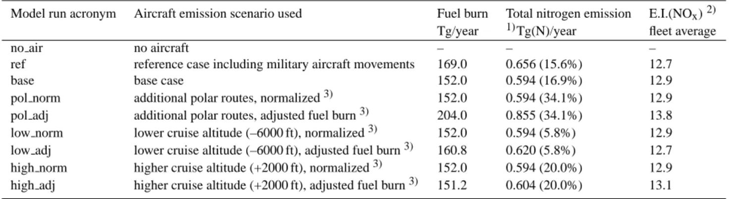
Table 1. Summary of the model simulations and TRADEOFF aircraft emission scenarios.

Model run acronym Aircraft emission scenario used Fuel burn Total nitrogen emission E.I.(NOx)2)

Tg/year 1)Tg(N)/year fleet average

no air no aircraft – – –

ref reference case including military aircraft movements 169.0 0.656 (15.6%) 12.7 base base case 152.0 0.594 (16.9%) 12.9 pol norm additional polar routes, normalized3) 152.0 0.594 (34.1%) 12.9 pol adj additional polar routes, adjusted fuel burn3) 204.0 0.855 (34.1%) 13.8 low norm lower cruise altitude (–6000 ft), normalized3) 152.0 0.594 (5.8%) 12.9 low adj lower cruise altitude (–6000 ft), adjusted fuel burn3) 160.8 0.620 (5.8%) 12.7 high norm higher cruise altitude (+2000 ft), normalized3) 152.0 0.594 (20.0%) 12.9 high adj higher cruise altitude (+2000 ft), adjusted fuel burn3) 151.2 0.604 (20.0%) 13.1 1) The fraction of aircraft emissions occurring in the stratosphere is given in parenthesis (see Sect. 4.2).

2) The NOxemission index, E.I.(NOx), is defined as grams of NOx(as NO2)emitted per kg of burnt fuel.

3) Changes in flight routing will in general imply changes in fuel burn. In the “adjusted fuel burn” cases this effect is taken into account, while the “normalized” scenarios use the same total fuel burn as in the “base” case.

−150 −100 −50 0 50 100 150 −60 −40 −20 0 20 40 60 80 2000 0 1 2 3 4 5 6

Fig. 1. Geographical distribution of aviation fuel burn in the TRADEOFF reference case (year 2000), vertically integrated for each 1◦×1◦column. Unit: log10[kg(fuel)/(day*1◦×1◦column)].

index, E.I.(NOx), equal to grams of NOx(as NO2)in the

ex-haust per kilograms of fuel burned. In the TRADEOFF refer-ence case for the year 2000, which is used in model run “ref” (see Table 1), both civil and military aircraft are included with a global annual fuel consumption of about 169 Tg and a global annual nitrogen emission of 0.656 Tg(N)/year, cor-responding to an average E.I.(NOx)of 12.7. The

geographi-cal distribution of the annual fuel consumption according to this scenario is plotted in Fig. 1, revealing peak emissions in the North Atlantic Flight Corridor, in North America, Eu-rope and the Far East. Using the NCEP tropopause height in

CTM2, about 16% of the global annual NOx output from

aviation is deposited directly into the stratosphere. How-ever, this fraction is strongly dependent on season and lati-tude due to variations in tropopause height. At low latilati-tudes, where the tropopause is high, aircraft operations occur en-tirely within the troposphere, while at high latitudes nearly all aircraft emissions are injected into the stratosphere. In mid-latitudes the tropopause height tends to be higher dur-ing summer leaddur-ing to a somewhat smaller fraction of strato-spheric emissions than during winter. This in reasonable agreement with what was found by Gettelman et al. (1999), who used both dynamical and thermal tropopause definitions for their analysis of the direct deposition of subsonic aircraft emissions into the stratosphere.

The novelty for the TRADEOFF work was the creation of seven scenarios for the investigation of the impact of po-lar routes and differing cruise altitudes: One base case and six perturbation cases. In contrast to the reference scenario (“ref”) these scenarios do not include military aircraft. In the TRADEOFF base case (labeled “base”), which corre-sponds to “ref” but excludes military aircraft, the global annual fuel consumption and nitrogen emission amount to about 152 Tg(fuel)/year and 0.594 Tg(N)/year. This dataset compares very well with more recent scenarios that were developed for the years 2000 and 2002, and also neglect military aircraft: 1) the “FAST-2000” inventory, which is based on actual flight movements of year 2000 and yields 152 Tg(fuel)/year and 0.618(N)/year, and 2) the AERO2K in-ventory, which represents year 2002 emissions and is used in the European Commission QUANTIFY Project. AERO2K yields 156 Tg(fuel)/year and 0.627 Tg(N)/year. Both inven-tories are described in Lee et al. (2005).

In two of the perturbation cases a selection of already ex-isting polar routes was substantially enhanced in order to in-vestigate the impact of increased polar routing. The first one

(model run “pol norm”) is normalized with respect to the “base” case, i.e. polar flights come as replacement of flights in lower latitudes and the global annual fuel burn and nitro-gen emission are identical to those in the “base” case. In the second one (model run “pol adj”), the enhanced polar routing comes in addition to conventional traffic, so that the global annual fuel consumption and nitrogen emission are substantially larger than in the “base” case. Also, the frac-tion of emissions occurring in the stratosphere is much larger in the polar route scenarios, reflecting the low tropopause height in high latitudes. The variation of E.I.(NOx)seen in

Table 1 is a “real” effect in the inventories. In case “pol adj”, the frequency of a small number of routes that goes near the pole (a particular subset of aircraft types) is magnified. By doing this, the overall inventory E.I.(NOx)changes as a

re-sult of changing the “population” of aircraft in the inventory. The four remaining scenarios addressed changes in cruis-ing altitude. In order to represent increased and decreased flight altitudes, increments of real flight levels were chosen, i.e. +2000 feet and –6000 feet (+610 m and –1830 m, respec-tively). The altitude decreases were specified by aircraft type and by mission distance. For the altitude increase some air-craft types for particular mission distances could not perform the flight. Thus, for this latter case, shifts in altitude were made only when feasible.

In the scenarios used for model runs “low norm” and “low adj”, the flight altitude is reduced. Again the first sce-nario features the same global annual fuel consumption and nitrogen emission as the “base” case, while in the second one, changes in fuel consumption and nitrogen emissions are taken into account. This approach reflects the impact resulting from alternative flight routing in a more realistic way than the normalized scenarios. Moreover, it allows for a separate calculation of the impacts of changed emission al-titude on the one hand and the concomitant change in fuel consumption on the other. As today’s cruise altitudes are determined by fuel efficiency considerations, a decrease of 6000 ft in cruise altitudes will lead to an increase in fuel con-sumption related to increased drag. Accordingly, the total NOxemission is slightly larger compared to the “base” case.

A considerable reduction is seen in the fraction of emissions released into the stratosphere, which in this case amounts to only 5.8% compared to 16.9% in the “base” case.

Finally, the emission scenarios applied in model runs “high norm” and “high adj” address an altitude increase of 2000 ft (610 m). A 2000 feet altitude increase is calculated to lead to a decrease in fuel consumption by 0.5% (owing to reduced drag), but to an increase in NOxemission of 1.6%.

This is due to the fact that those aircraft types that can fly 2000 feet higher have a higher average E.I.(NOx)at this

al-titude. In model run “high adj” these changes are taken into account, while in model run “high norm” the global annual fuel consumption and nitrogen emission are the same as in the “base” case run. Figure 2 shows the vertical distribution of aircraft NOxemissions in the “base” case and the four

sce-0 0.05 0.1 0.15 0.2 0.25 6.71 7.32 7.93 8.54 9.15 9.76 10.37 10.98 11.59 12.20 12.81 Tg(N)/(year*layer)

height of layer boundary (km) base_{low_norm} low_adj high_norm high_adj

Fig. 2. Total annual NOxinjection into flight levels between 6710 m

and 12 810 m according to the TRADEOFF scenarios “base”, “low norm”, “low adj”, “high norm”, and “high adj” (see Table 1), plotted as Tg(N)/(year*610 m-layer). Thin horizontal lines depict flight level boundaries.

narios dealing with changes in flight altitude. As not all air-craft types are able to fly at higher altitudes the emissions in the altitude range with maximum “base” case traffic (10.37– 10.98 km) is still large in the higher altitude scenarios, albeit reduced. By contrast, in the lower altitude scenarios no emis-sions occur in this region. The meteorology in all model sim-ulations of this study is taken from ECMWF short-term (12– 36 h) forecast data for the year 2000, which have been found to be better suited for the model than reanalyzed data. First, a five-year model spin-up is performed without aircraft to pro-vide an initial condition for the 3-dimensional fields of all modeled chemical species. Starting from this initial condi-tion, follow-up runs are integrated for three additional years without aircraft emissions and with aircraft emissions ac-cording to the various scenarios described above. The emis-sions and tropospheric boundary conditions used are sum-marized in Table 2. Surface emissions of CH4 in the year

2000 are mimicked by setting a constant mixing ratio in the lowermost 5 layers of CTM2 (up to about 200 m). 1790 and 1700 ppbv are chosen in the Northern and Southern Hemi-spheres, respectively.

Table 2. Emissions and boundary conditions used in the model simulations.

Species Mixing ratio/emission CH4 1745 ppbv

CO 547 Tg(CO)/year VOC 133 Tg(C)/year NOx– Biofuel 2.41 Tg(N)/year

NOx– Fossil Fuel 25.55 Tg(N)/year

NOx– Industry 2.01 Tg(N)/year

NOx– Biomass burning 5.84 Tg(N)/year

NOx– Soils 8.01 Tg(N)/year

NOx– Lightning 5.00 Tg(N)/year

NOx– Aircraft 0.59 – 0.71 Tg(N)/year (depending on scenario)

N₂O 318 ppbv Cly (ETCL)1) 3.54 ppbv Bry (ETBL)2) 16.34 pptv 1) Equivalent Tropospheric Chlorine Loading (WMO, 1999). 2) Equivalent Tropospheric Bromine Loading (WMO, 1999).

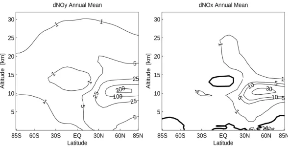
85S 60S 30S EQ 30N 60N 85N 5 10 15 20 25 30 Latitude Altitude [km]

dNOy Annual Mean

1 1 1 1 1 5 5 5 25 25 25 100200 85S 60S 30S EQ 30N 60N 85N 5 10 15 20 25 30 Latitude Altitude [km]

dNOx Annual Mean

−1 −1−1 1 1 1 1 1 5 5 ₅ 10 10 30

Fig. 3. Annually averaged changes in zonal-mean NOy(left) and NOx(right) due to aircraft emissions in the TRADEOFF reference case,

i.e. “ref minus no air” (units: pptv). Contours at –1, 0, 1, 5, 25, 100, 200 for NOy, and –1, 0, 1, 5, 10, 30 for NOx.

4 Results

4.1 Impact of aircraft emissions in the tradeoff reference case

Model simulations “no air” and “ref” are performed to as-sess the overall effect of NOx emissions from aircraft,

in-cluding military aircraft. Figure 3 shows annually averaged zonal-mean changes in NOy, i.e. total reactive nitrogen,

de-fined as the sum of NO, NO2, NO3, N2O5, HNO4, ClONO2,

BrONO2, HNO3, and PAN, and in NOx, which is the sum

of NO and NO2, due to military and civil aircraft emissions

in the year 2000. Notable perturbations are confined to the

Northern Hemisphere, reflecting the asymmetric distribution of aircraft emissions, with maximum increases amounting to 212 pptv for NOyand 45 pptv for NOx. In CTM2 most of

the NOy increase is present as HNO3, as is apparent from

the much smaller NOx increases. Small decreases of

near-surface NOxare modeled in some areas, probably related to

increases in ozone, which converts NOxinto NOy as found

in earlier aircraft studies (Stevenson et al. 1997). Regard-ing the seasonal variation and locations of the maximum per-turbation (not shown), NOyis substantially enhanced during

winter and spring with maximum increases between 250 and 300 pptv in the tropopause region in high Northern latitudes. In CTM2 this corresponds to a relative increase of about

Table 3. Changes in the total ozone column and, in parenthesis, the tropospheric ozone column, averaged over the globe and over the

Northern Hemisphere in the various model simulations discussed in this and the following sections (units: DU). In order to obtain ozone burden change in Tg, global averages and Northern Hemisphere averages (in DU) have to be multiplied by 10.93 Tg/DU and 5.47 Tg/DU, respectively.

Model run accronym Global average: Northern Hemisphere average:

δtotal ozone (DU) δtotal ozone (DU) δtotal ozone (DU) δtotal ozone (DU) with respect to with respect to with respect with respect the “no air” case the “base” case to the “no air” case to the “base” case ref +0.39 (+0.33) +0.68 (+0.58) base +0.34 (+0.29) +0.59 (+0.50) pol norm +0.33 (+0.27) –0.01 (–0.02) +0.59 (+0.48) +0.00 (–0.02) pol adj +0.45 (+0.37) +0.11 (+0.08) +0.81 (+0.66) +0.21 (+0.16) low norm +0.31 (+0.29) –0.03 (–0.00) +0.55 (+0.50) –0.04 (+0.00) low adj +0.33 (+0.30) –0.01 (+0.01) +0.57 (+0.52) –0.02 (+0.02) high norm +0.35 (+0.29) +0.01 (+0.00) +0.60 (+0.50) +0.01 (+0.00) high adj +0.35 (+0.30) +0.02 (+0.01) +0.61 (+0.51) +0.02 (+0.01)

40%. Throughout the year the maximum increase in zonal-mean NOyis located in mid- to high Northern latitudes

be-tween 10 and 12 km. During Northern Hemisphere Summer and in January the maximum increase is located at the North Pole (the northernmost latitude belt of CTM2 is centered at about 86 degrees N). In July and October the increases are al-most twice as small but still pronounced. The seasonal varia-tion of NOyperturbations is mainly related to meteorological

conditions, in particular the height of the tropopause, which is low in high Northern latitudes during winter allowing air-craft emissions to accumulate more efficiently, and convec-tive transport and washout of NOyin the troposphere. In

par-ticular during July, August, and September convective activ-ity and thus vertical mixing and washout processes in the tro-posphere are relatively vigorous in CTM2 leading to smaller maximum increases in NOyat mid latitudes, as was already

found in earlier CTM2 studies (Kraabøl et al., 2002). Thus the relatively smaller increase in high latitudes represents the maximum increase in NOyduring these months. Maximum

increases in NOxrange from about 40 to almost 70 pptv,

de-pending on season. At night and at large solar zenith angles, the NOx/NOyratio is low, leading to a notable displacement

of the maximum NOx increase towards the equator during

Northern Hemisphere winter.

The annual average of zonal-mean ozone and OH changes is shown in Fig. 4. The maximum increase in ozone is located in high Northern latitudes and amounts to 4.3 ppbv, while the maximum increase in OH is seen in mid Northern latitudes reaching 9.4×104molecules cm−3. Above about 20 km al-titude in high southern laal-titudes ozone is slightly reduced through catalytic NOx cycles, although this perturbation is

not pronounced. Regarding OH, NOx emissions lead to a

slight enhancement through the reaction of NO and HO2and

the increase of ozone, which is an OH precursor. Above a

certain height in the lower stratosphere, however, decreases in OH are modeled, albeit very small. This is probably con-nected to the reactions of HNO3 and HO2NO2 with OH,

which gain importance in the stratosphere in mid- to high latitudes in their competition with OH-producing reactions. The magnitude and latitude of the maximum ozone increase are plotted in Fig. 5. Owing to the close link between sun-light and ozone chemistry, the figure exhibits a strong sea-sonal variation. Maximum increases are seen during periods coinciding with low solar zenith angles, i.e. late spring and summer. The maximum is located in the northernmost lat-itude belt during summer, when the sun is present all day, while in winter it is displaced towards the equator, as far as 40 degrees North in the period December to February. The very high latitude of maximum increases during summer is explained by enhanced convective activity during summer, which reduces the ozone increase in mid-latitudes. Excess ozone produced from NOxemissions in the UTLS is

trans-ported into the lower troposphere where the chemical life-time of ozone is shorter and where it is lost through dry de-position.

The maximum zonal-mean increase in ozone is modeled in June amounting to nearly 8 ppbv, coincident with maxi-mum actinic flux. Relatively small ozone increases between 3 and 4 ppbv are modeled between September and January, resulting from a combination of less sunlight and lower NOy

perturbations due to meteorological conditions.

Table 3 lists changes in total ozone for all perturbations discussed in this paper. For the increase due to aircraft in the TRADEOFF reference case (“ref”) with respect to the “no air” simulation a global mean increase of about 0.39 DU is modeled, corresponding to an ozone burden in-crease of 4.24 Tg. For the Northern Hemisphere these values are 0.68 DU and 3.72 Tg, i.e. most of the increase in ozone

85S 60S 30S EQ 30N 60N 85N 5 10 15 20 25 30 Latitude Altitude [km]

dO3 Annual mean

0.1 0.1 0.1 0.1 0.1 0.1 0.5 0.5 0.5 1 1 2 2 3 4 85S 60S 30S EQ 30N 60N 85N 5 10 15 20 25 30 Latitude Altitude [km]

dOH Annual mean

−0.1 −0.1 0.1 0.1 0.1 0.1 0.1 1 1 1 1 3 3 75

Fig. 4. Annually averaged changes in zonal-mean ozone (ppbv) and OH (104molecules cm−3)due to aircraft emissions in the TRADEOFF reference case, i.e. “ref minus no air”. Contours at: –0.1, 0, 0.1, 0.5, 1, 2, 3, 4 for ozone and –1, –0.1, 0, 0.1, 1, 3, 5, 7, 9 OH.

3 4 5 6 7 8

Zonal−mean ozone perturbation

ppbv

JAN FEB MARAPR MAY JUN JUL AUG SEP OCT NOVDEC40 50 60 70 80 90 degrees North magnitude of max latitude of max

Fig. 5. Maximum increase in monthly averaged zonal-mean ozone due to aircraft in the TRADEOFF reference case as a function of season,

i.e. “ref minus no air”. Solid line: magnitude of the maximum (ppbv, left axis), dashed line: latitude at which the maximum increase occurs (degrees North, right axis).

burden is located in the Northern Hemisphere. Values for changes in the tropospheric ozone column are listed in paren-thesis. It is seen that most of the increase in the TRADEOFF reference case occurs in the troposphere. Concerning ozone column change, both the tropospheric and the total (i.e. sur-face to CTM2 lid) ozone columns are modeled to increase in all seasons and all latitudes. The maximum tropospheric and total column increases are modeled in mid- to high Northern Latitudes during May and amount to 1.15 DU (2.52%) and 1.34 DU (0.35%), respectively.

The results of this study can not easily be compared quan-titatively with earlier studies, because new aircraft emission scenarios are used here. However, the spatial distribution and seasonal variation of NOxand ozone changes are similar to

what was obtained in earlier studies (Wauben et al., 1997;

Stevenson et al., 1997; Berntsen and Isaksen, 1999; Kentar-chos and Roelofs, 2002). K¨ohler et al. (1997) obtained max-imum zonal-mean NOxincreases exceeding 50 pptv in both

January and July, i.e. somewhat larger than in the present study. This is due to the larger emission source used in their study (i.e. 0.85 Tg(N)/yr), but also to plume chem-istry processes reducing both NOy and NOx perturbations

in our study. Compared to the results of Kentarchos and Roelofs (2002), who used a total aircraft emission source of 0.56 Tg(N)/yr, our maximum ozone increase is further North in July and larger in magnitude, while the perturbations in NOxare in approximate agreement, especially in January

(al-though it has to be noted that Kentarchos and Roelofs include HNO4, NO3 and N2O5in the definition of their NOx). In

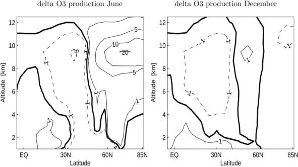
delta O3 production June delta O3 production December EQ 30N 60N 85N 2 4 6 8 10 12 Latitude Altitude [km] −5 −1 −1 −1 −1 −1 1 1 1 5 5 10 20 EQ 30N 60N 85N 2 4 6 8 10 12 Latitude Altitude [km] −1 −1 −1 −1 −1 1 1

Fig. 6. Change in net chemical ozone production (103molecules/cm−3s−1)due polar routes replacing conventional routes, i.e. “pol norm minus base” in June (left) and December (right). Contours at –5, 1, 0, 1, 5, 10, and 20.

on Aviation and the Global Atmosphere (Penner et al., 1999) and the final report of the TRADEOFF project (Isaksen, 2003), uncertainties between the models concerning ozone change appear quite large, but the results obtained in our study are well within the uncertainty range of the model-ing community. For example, in Penner et al. (1999, their Fig. 4-1) upper tropospheric ozone increases modeled for 2015 are typically in the range 5–10 ppbv, which compares well with the 4–5 ppbv obtained in our study, considering that the global aircraft NOxemission source is estimated about a

factor of two smaller in 2000 (0.65 Tg(N)/year) than what was used in Penner et al. (1999) for 2015 (1.25 Tg(N)/year). The same is true for perturbations in NOx, which amount to

about 45 ppbv at maximum in our study (Fig. 3) compared to 60–150 ppbv in the IPCC (1999, their Fig. 4-2) models for 2015 using a doubled emission total. What is new in the present study with respect to IPCC (1999) is that we are using a model including both tropospheric and stratospheric chem-istry, rather than prescribing stratospheric boundary condi-tions. In particular, both the ozone reducing effect from cat-alytic NOx cycles and the ozone producing effect of NOx

emissions in the lower stratosphere are included in the our model stratosphere. The ozone depleting effect reveals itself in Fig. 4 in the Antarctic stratosphere, although this effect is negligible compared to the ozone producing effect of NOx

emissions at lower altitudes.

4.2 Tradeoffs in enhanced polar routing

Six TRADEOFF scenarios were designed for comparison with the TRADEOFF base case (“base”), not including

mili-tary aircraft: two scenarios addressing polar routes and four dealing with changes in flight altitudes. The impact of air-craft emissions in the “base” case simulation is qualitatively the same as in the reference case (“ref”), which includes mil-itary aircraft and was discussed in the previous section. Due to the lower emission rate, however, the magnitudes of in-crease are slightly smaller, which is why the following dis-cussion focuses on the relative change of aircraft impact due to flight routing rather than the aircraft impact itself.

In recent years polar routes in the Northern Hemisphere have been increasingly used by long range aircraft. For in-stance, great circle (i.e. shortest) connections between city pairs in Europe and the Western part of North America or be-tween the Far East and the Eastern part of North America go through Arctic regions, and are/will be followed by airlines as closely as possible. Within TRADEOFF the impact of in-creased polar routing has been studied by enhancing already existing polar routes in the Northern Hemisphere signifi-cantly and by analyzing the model response. The polar envi-ronment differs from the mid-latitude regions because of the relatively low tropopause height, implying a larger fraction of the flight operations occurring in the stratosphere. This, in turn, implies a less efficient removal of NOx pollutants

through wash-out at cruise altitudes. Also, the strong de-pendence of chemistry on sunlight combined with the strong seasonality of insolation in high latitudes lead to a large sea-sonal variability in ozone impact due to aircraft in high lat-itudes, which is of particular importance when considering increased high latitude routing. Figure 6 shows the change in net chemical production due to polar routing replacing stan-dard routes. In June the impact is clearly revealed, while in

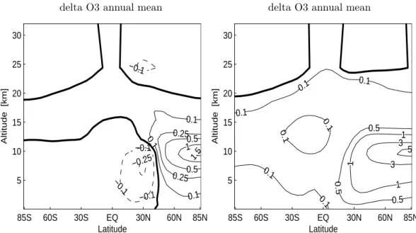
delta O3 annual mean delta O3 annual mean 85S 60S 30S EQ 30N 60N 85N 5 10 15 20 25 30 Latitude Altitude [km] −0.25 −0.1 −0.1 −0.1 −0.1 0.1 0.1 0.1 0.25 0.25 0.5 0.5 1 1.5 85S 60S 30S EQ 30N 60N 85N 5 10 15 20 25 30 Latitude Altitude [km] 0.1 0.1 0.1 0.1 0.1 0.1 0.1 0.5 0.5 0.5 1 1 1 3 3 5

Fig. 7. Annually averaged zonal-mean ozone change (ppbv) due to polar routes replacing conventional routes (left panel, “pol norm minus

base”) and the total impact due to aircraft emissions in the normalized polar route scenario (right panel, “pol norm minus no air”). Contours at –0.25, –0.1, 0, 0.1, 0.25, 0.5, 1, 1.5, 3, and 5 (in the right panel the 0.25 and 1.5 contours are omitted).

December in the absence of sunlight in high Northern lati-tudes, it is negligible. The slight decrease in mid-latitudes in this perturbation results from a reduction in mid-latitude traf-fic in this scenario. Annually averaged zonal-mean changes in ozone for the “pol norm” simulation are presented in Fig. 7 with respect to the “base” and the “no air” simula-tions. In the middle stratosphere signs of ozone depletion due to NOx emissions are seen, but this effect is negligible

in view of the large ambient ozone levels in these altitudes. The decrease of conventional routes manifests itself by the reduced ozone increase in mid- and low Northern latitudes in the troposphere with respect to the “base” case. The ozone impact with respect to the “no air” case reveals appreciable increases in the Arctic up to an altitude of about 20 km. Max-imum increases in the Arctic UTLS region with respect to the “no air” simulation exceed 5 ppbv, which is more than 30% larger a perturbation than is obtained in the “base” case.

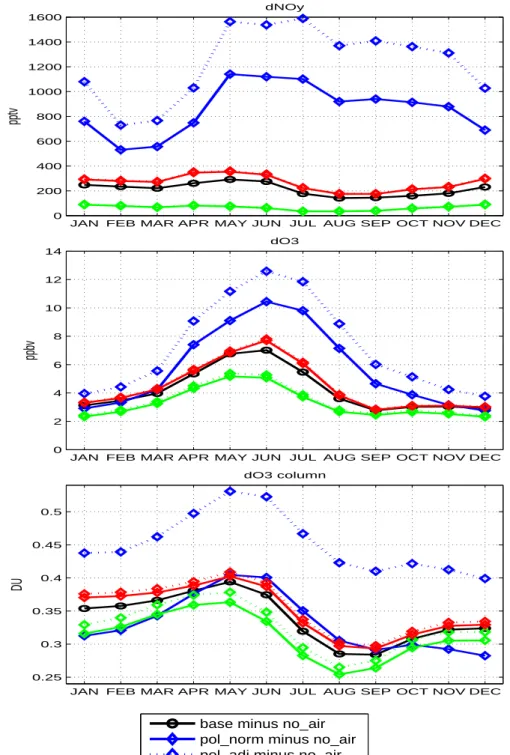
Figure 8 shows the seasonal variations of the maximum zonal-mean increases in NOy and ozone, together with the

global average increase in total ozone for the polar route sce-narios (blue lines) and the other TRADEOFF scesce-narios to be discussed in Sect. 4.3 (red and green lines), along with the “base” case perturbation (black line). As shown by the blue lines in the upper panel of the figure, NOy increases

drasti-cally in the polar route scenarios since washout of HNO3is

less important in high latitudes and absent in the lower strato-sphere, in which most of the additional high latitude emis-sions occur. The latitude of the maximum NOyincrease (not

shown) is north of 80◦N throughout the year. The maximum increase in zonal-mean ozone (blue line in the middle panel)

is strongly influenced by solar radiation, which is a maxi-mum during summer. As the seasonal variation of actinic flux is particularly strong in high latitudes the seasonality of the maximum ozone increase is much more pronounced than in the “base” case. Indeed, in the normalized polar route scenario during winter, zonal mean increases in ozone are even smaller than in the “base” case. This is even more pro-nounced in the total ozone increase shown by the blue lines in the bottom panel of the figure. In the Northern Hemisphere, a replacement of conventional routes by polar routes would re-duce the impact on the tropospheric column and increase the stratospheric column on an annual average since more emis-sions occur in the lower Arctic stratosphere. In the South-ern Hemisphere both the increases in tropospheric and strato-spheric columns are reduced with respect to the “base” case, as no high Southern latitude routes are introduced. Judging by the increase in global ozone burden only, a replacement of conventional routes by polar routes would reduce the envi-ronmental impact of aircraft with respect to the “base” case. However, this tradeoff is very small and subject to meteoro-logical conditions such as washout and tropopause height in the Arctic regions, which are subject to interannual variation. Concerning ozone column change due to polar rout-ing replacrout-ing standard routes (“pol norm minus base”), the aircraft-induced increase in both tropospheric and total ozone columns is reduced in low Northern latitudes due to the pole-ward shift of aircraft emissions. Substantial increases are confined to the summer season in high Northern latitudes. Regarding the ozone burden, the increases in ozone in high latitudes are not compensated by reductions in mid- and low

JAN FEB MAR APR MAY JUN JUL AUG SEP OCT NOV DEC 0 200 400 600 800 1000 1200 1400 1600 pptv dNOy

JAN FEB MAR APR MAY JUN JUL AUG SEP OCT NOV DEC 0 2 4 6 8 10 12 14 ppbv dO3

JAN FEB MAR APR MAY JUN JUL AUG SEP OCT NOV DEC 0.25 0.3 0.35 0.4 0.45 0.5 dO3 column DU

base minus no_air pol_norm minus no_air pol_adj minus no_air low_norm minus no_air low_adj minus no_air high_norm minus no_air high_adj minus no_air

Fig. 8. Maximum zonal-mean NOyincrease (upper panel, pptv), maximum zonal-mean ozone increase (middle panel, ppbv), and globally

averaged ozone column increase (bottom panel, DU) as a function of season for different TRADEOFF simulations with respect to the “no air” run.

delta NOy annual mean delta NOx annual mean EQ 30N 60N 85N 0 2 4 6 8 10 12 Latitude Altitude [km] −10 −10 −10 −8 −8 −8 −8 −6 −6 −6 −6 −6 −4 −4 ₋₄ −2 −2 −2 −2 −2 2 2 EQ 30N 60N 85N 0 2 4 6 8 10 12 Latitude Altitude [km] −2 −2 −1.5 −1.5 −1 −1 −1 −1 −1 −0.5 −0.5 −0.5 −0.5 0.5 0.5 1

Fig. 9. Annual-mean changes in concentrations of NOy(top left, 108molecules/cm−3)and NOx(top right, 108molecules/cm−3)in the

Northern Hemisphere due to a 1830 m reduction in flight altitude taking into account changes in fuel consumption, i.e. “low adj minus base”. Contours at –12, –10, –8, –6, –4, –2, 0, 2 for NOyand –2.5, –2, –1.5, –1, –0.5, 0, 0.5, 1 for NOx.

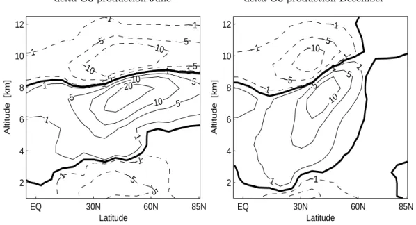
delta O3 production June delta O3 production December

EQ 30N 60N 85N 2 4 6 8 10 12 Latitude Altitude [km] −10 −10 −5 −5 −5 −5 −5 −5 −5 −1 −1 −1 −1 −1 −1 −1 −1 1 1 1 1 5 5 5 10 10 20 EQ 30N 60N 85N 2 4 6 8 10 12 Latitude Altitude [km] −10 −5 −5 −1 −1 −1 −1 −1 ₁ 1 1 5 5 10

Fig. 10. Change in net chemical ozone production (103molecules cm−3s−1)due to a 1830 m reduction in flight altitude, taking into account changes in fuel consumption, i.e. “low adj minus base” in June (left) and December (right). Contours at –20, –10, –5, –1, 0, 1, 5, 10, and 20.

latitudes. With respect to the “no air” case, the increase in ozone burden in the “pol norm” scenario is thus substantially larger than in the “base” case.

4.3 Tradeoffs in changing flight altitude

Since the effects of aircraft NOx emissions exhibit strong

altitudinal dependencies, it has been suggested that the

air-craft impact can be reduced by changing flight altitude. Changes in flight altitude will generally lead to modifica-tions in the height profile of ozone change, with the impact getting smaller in certain height regions and larger in others. This is partly a direct consequence of changed distributions of aircraft emissions, but is also connected to the changes in the ambient conditions where the flights are operated. In

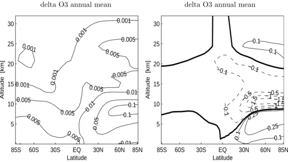
delta O3 annual mean delta O3 annual mean 85S 60S 30S EQ 30N 60N 85N 5 10 15 20 25 30 Latitude Altitude [km] 0.001 0.001 0.001 0.001 0.001 0.005 0.005 0.005 0.005 0.005 0.005 0.005 0.005 0.01 0.01 0.01 0.05 0.1 0.1 85S 60S 30S EQ 30N 60N 85N 5 10 15 20 25 30 Latitude Altitude [km] _−1.5 −1.5 −1.5 −1 −1 −0.5 −0.5 −0.5 −0.1 −0.1 −0.1 0.1 0.1 0.1 0.1 0.25 0.25

Fig. 11. Annually averaged zonal-mean ozone change (ppbv) due a 1830 m reduction in flight altitude. Left panel: “low adj minus

low norm”, i.e. separated effect of changes in fuel consumption, and right panel: “low adj minus base”, i.e. total effect of lowering the flight altitude.

particular, a higher cruise altitude will lead to a larger frac-tion of aircraft emissions occurring in the stratosphere where wash-out processes are largely absent and vertical motions are much slower. Thus NOxpollutants from aircraft can

ac-cumulate more efficiently leading to larger ozone perturba-tions. On the other hand ozone perturbations at lower alti-tudes become smaller as air traffic is reduced there. For the lower altitude scenarios the opposite is true. The key ques-tion to be addressed in this secques-tion is to what extent the neg-ative and positive effects cancel each other in terms of total ozone column change.

Not surprisingly, lowering the flight altitude reduces air-craft impact at standard flight altitudes, while increasing it at lower altitudes. Figure 9 shows the zonal-mean change in the concentrations of NOy and NOx due to a 1830 m

reduction in flight altitude taking into account changes in fuel consumption. In low to mid-Northern latitudes, we calculate decreases above 8 to 9 km altitude and in-creases below, which is a result of lowering the emission source. However, it is important to note that the increase at low altitudes is much smaller in magnitude than the de-crease at high altitudes, although the inde-crease in fuel con-sumption leads to a somewhat larger emission rate at the new altitude (the Figure shows changes in concentration rather than mixing ratios in order to make this relation clearer). In the case of NOy, maximum reductions are

modeled between 10 and 11 km altitude in Northern mid-latitudes, amounting to –11×108molecules/cm3, while the maximum increase between 6 and 8 km altitude remains below +3×108molecules/cm3. For NOx the

correspond-ing maximum changes are –2.5×108and +1.1×108, respec-tively. This asymmetry is, first and foremost, connected to washout of HNO3, which is much more efficient at low

alti-tudes, while being virtually absent in the lower stratosphere. The HOx partitioning (not shown) is shifted towards OH in

regions of enhanced NOxemissions, and towards HO2in

re-gions of reduced NOxemissions. In low latitudes, increases

in HO2are seen in the troposphere as well. These are regions

where HOxincreases as a whole due to the ozone increase.

As a result of these changes, the ozone net production, shown in Fig. 10, is enhanced below about 8 km, and reduced above. However, the effect is more pronounced during summer re-lated to larger photochemical activity. In particular, there is no reduction in chemical ozone production in the Arctic lower stratosphere during the winter season.

A normalized scenario for the lower flight altitude case was created to estimate the effect from changes in fuel con-sumption individually. Lowering the cruise altitude will in-crease air resistance because the air density inin-creases with decreasing altitude in the atmosphere. As a result, fuel con-sumption and NOxemissions will increase. Figure 11 shows

the separate effect of increasing fuel emission along with the total effect of reducing flight altitude on zonal-mean ozone. Although the magnitude of changes related to fuel consump-tion is much smaller than the total aircraft effect, it has to be noted that the increase covers all altitudes, i.e. there are no canceling effects between changes of opposite signs at dif-ferent altitudes. Therefore, in terms of total ozone change, the effect of increased fuel burn is large compared to the ef-fect from lowering the flight altitude alone.

delta NOy annual mean delta NOx annual mean EQ 30N 60N 85N 0 2 4 6 8 10 12 Latitude Altitude [km] −0.4 −0.2 −0.2 1 2 4 EQ 30N 60N 85N 0 2 4 6 8 10 12 Latitude Altitude [km] −0.2 −0.2 0.2 0.2 _0.2 0.4 0.4 _0.6 0.6 0.81

Fig. 12. Annual-mean changes in concentrations of NOy(top left, 108molecules cm−3)and NOx(top right, 108molecules cm−3)in the

Northern Hemisphere due to a 610 m increase in flight altitude taking into account changes in the total emission of nitrogen, i.e.“high adj minus base”. Contours at –0.4, –0.2, 0, 1, 2, 4 for NOyand –0.4, –0.2, 0, 0.2, 0.4, 0.6, 0.8, 1.0 for NOx.

delta O3 production June delta O3 production December

EQ 30N 60N 85N 2 4 6 8 10 12 Latitude Altitude [km] −1 −1 −1 −1 −1 −1 1 1 1 1 5 EQ 30N 60N 85N 2 4 6 8 10 12 Latitude Altitude [km] −1 −1 −1 −1 1 1 1

Fig. 13. Change in net chemical ozone production (103molecules cm−3s−1)due to a 610 m increase in flight altitude, taking into account changes in the total emission of nitrogen, i.e.“high adj minus base” in June (left) and December (right). Contours at –5, –1, 0, 1, 5.

As shown in Table 3, the total increase in the “base” case is +0.339 DU (+3.71 Tg). Reducing flight altitude alone (“low norm minus base”) leads to a decrease of – 0.0266 DU (–0.29 Tg) and increasing fuel use (“low adj minus low norm”) to +0.0131 DU (+0.14 Tg), so that the total increase due to aircraft in the lower flight altitude scenario (“low adj minus no air”) amounts to +0.3255 DU

(+3.56 Tg). These findings are in qualitative agreement with the results in a similar study of Grewe et al. (2002b), while the magnitudes of change cannot easily be compared because of the larger total emission from aircraft and the smaller al-titude decrease considered in the Grewe et al. study. Also, it has to be noted that the effect on column ozone is strongly dependent on both season and latitude, as reflected by the

delta O3 annual mean delta O3 annual mean 85S 60S 30S EQ 30N 60N 85N 5 10 15 20 25 30 Latitude Altitude [km] 0.001 0.001 0.001 0.001 0.005 0.005 0.005 0.005 0.005 0.01 0.01 0.01 0.05 85S 60S 30S EQ 30N 60N 85N 5 10 15 20 25 30 Latitude Altitude [km] −0.05 −0.05 −0.05 −0.05 0.05 0.05 0.05 0.05 0.05 0.1 0.1 0.4_0.4

Fig. 14. Annually averaged zonal-mean ozone change (ppbv) due a 610 m increase in flight altitude. Left panel: “high adj minus high norm”,

i.e. separated effect of changes in fuel consumption, and right panel: “high adj minus base”, i.e. total effect of increasing the flight altitude.

varying gap between the green dotted and the solid black lines in Fig. 8 (lower panel) and the latitudinal distribution of total ozone change (not shown). The reduction in flight altitude leads to decreases in the tropospheric ozone col-umn in low latitudes, which is a clear manifestation of the importance of washout processes. Both in the “base” case and in the lower-altitude case, virtually all low-latitude air-craft traffic is located in the troposphere, and the lowering of the aircraft emission source results in a larger fraction of emitted nitrogen emissions to be washed out. In contrast, an increase in the tropospheric ozone column is modeled at mid- to high Northern latitudes for the lower-altitude sce-nario (“low adj”). This is due to the enhanced fuel use, and the larger fraction emitted in the troposphere with respect to the “base” case. However, this increase is overcompen-sated by a corresponding stratospheric decrease during sum-mer and mid-winter so that the total ozone column change is negative in these seasons, as it is in all seasons at low lati-tudes. During summer the main reason for this is the high tropopause. A large fraction of aircraft emissions is occur-ring in the troposphere so that the increase of washout pro-cesses and the decrease of ozone lifetime with decreasing altitude are important. On the other hand, during spring and autumn the tropopause tends to be lower and even in the low altitude scenario a very large fraction of aircraft emissions occurs in the stratosphere, where washout does not play a role. The other effect, i.e. the decrease in residence times of pollutants in the lower stratosphere with decreasing altitude is not sufficiently important to compensate for the increases in the troposphere. The effect on the total column is thus positive, albeit only slightly. The next option, an increase in

flight altitude by 610 m, is investigated through model runs “high norm” and “high adj”. Figure 12 shows annually aver-aged zonal-mean changes in the concentrations of NOyand

NOxdue to a 610 m increase in flight altitude taking into

ac-count changes in fuel consumption and in the total emission of nitrogen. In Northern mid- to high latitudes we calcu-late increases above 8 to 9 km altitude and decreases below. Again, the effect at high altitudes is larger in magnitude than the effect at low altitudes. For instance, the maximum (high altitude) increase in NOy amounts to +4.5×108 molecules,

while the magnitude of the largest reduction is about ten times smaller, –0.43×108molecules/cm3. This can be in part explained by less efficient washout of excess NOyat the new

(and higher) altitude of emission. Also, the longer efflu-ent lifetime at higher altitudes allows for more pronounced increases and thereby to increased downward flux of NOy,

which partly compensates for the reduced in situ NOx

emis-sions at lower altitudes. Maximum changes in NOxand NOy

are displayed in Fig. 8. Slightly larger perturbations are ob-tained compared to the “base” case, with the fuel consump-tion effect being of minor importance.

By and large, increases of the OH/HO2ratio (not shown)

are seen in regions where the NOx emission is enhanced,

while reductions in NOxemissions are marked by lower OH

and higher HO2 concentrations. Qualitatively, the effect of

higher flight altitude is approximately opposite from what is obtained in the lower-altitude simulations. However, the magnitude of the effect is somewhat smaller, primarily be-cause the change in flight altitude is smaller. The same is true for changes in the chemical net production, which is shown in Fig. 13. The tendency is a reduction below about 8 to

−6000 −5000 −4000 −3000 −2000 −1000 0 1000 2000 −0.05 −0.04 −0.03 −0.02 −0.01 0 0.01 0.02 0.03

change in cruise altitude [feet]

[DU]

delta O3 column

low_norm − base − high_norm (trop) low_adj − base − high_adj (trop) low_norm − base − high_norm (strat) low_adj − base − high_adj (strat)

Fig. 15. Change in the Northern Hemisphere average tropospheric and stratospheric ozone columns (DU) due to changes in flight altitude,

based on the numbers given in Table 4. The increase in the “base” run is set to zero. E.g., the thin dashed line depicts the 0.0221 DU increase in tropospheric ozone column in simulation “low adj” with respect to “base” (at –6000 feet) and the 0.0080 DU increase in the tropospheric ozone column in simulation “high adj” with respect to “base” (at +2000 feet).

10 km, and an enhancement above, which is again most pro-nounced during summer, as it was in the lower-altitude case (Fig. 10).

Figure 14 shows the individual effect of changes in fuel consumption and the overall effect of increasing the flight altitude on zonal-mean ozone. The effect of the increased NOx emissions from fuel burn enhancement is positive at

all altitudes, while the overall effect is slightly negative at low altitudes, positive in the lower stratosphere and again negative in the middle stratosphere, probably due to ozone depletion mechanisms involving NOx, which is increased at

this altitude with respect to the “base” case run. As seen in Table 3 the overall effect on the ozone column due to in-creased flight altitude is positive both in the stratosphere and in the troposphere. Through the increase in flight altitude the ozone increase is enhanced by 0.0103 DU (0.11 Tg) globally (“high adj minus base”), while the increase in NOxemission

due to the higher E.I.(NOx)contributes another 0.0054 DU

(0.06 Tg) (“high adj minus high norm”), so that the overall effect increase represented by the difference “high adj minus base” amounts to 0.0157 DU (0.17 Tg). Averaged over the Northern Hemisphere the increase equals 0.0207 DU, corre-sponding to a 0.11 Tg increase of the hemispheric burden.

The effect on the globally averaged ozone column is de-picted by the red lines in Fig. 8 (bottom panel).

Concern-ing the latitudinal and seasonal variation of ozone column change (not shown), the results are, by and large, opposite in sign to what is obtained for a reduction in flight altitude. In the Southern Hemisphere and in low latitudes of the North-ern Hemisphere, there is an increase in both the tropospheric and the stratospheric columns. In mid- to high latitudes the effect on the tropospheric column is negative because of the relatively low tropopause causing a large reduction in tropo-spheric emissions in the high-altitude scenario. By contrast, due to the high summer tropopause a large fraction of emis-sion occurs in the troposphere even in the high altitude sce-nario allowing for increases in the ozone impact related to less efficient washout of pollutants. The effect of enhanced flight altitudes on the total ozone column is positive almost everywhere, except for high Northern latitudes in December. As this exception occurs in the absence of sunlight, it must be related to transport of air that is poorer in ozone compared to the “base” case.

In Fig. 15 the dependence of changes in tropospheric and stratospheric ozone columns on flight altitude is visu-alized relative to the changes calculated for the “base” case. The perturbations due to a 6000-feet reduction in flight al-titude are positive for the tropospheric and negative for the stratospheric ozone columns, which is a consequence of in-creased tropospheric and reduced stratospheric emissions,

respectively. The increase in tropospheric columns is much more pronounced when the increased fuel emission is taken into account.

A 2000-feet increase in flight altitude leads to increases in both the tropospheric and the stratospheric ozone column. Increases in the stratosphere are a direct consequence of in-creased emissions, while increases in the troposphere are mostly due to increased downward transport of NOyand

re-sulting increases in tropospheric ozone production.

5 Conclusions and future directions

In this paper we have presented results from an extensive model study performed for the TRADEOFF project focusing on the environmental impact of aircraft emissions and op-tions to reduce the impact for present condiop-tions (year 2000) and on the impact of aircraft emissions in a future (year 2050) atmosphere. We have used a 3-D chemical transport model including comprehensive chemistry schemes for the tropo-sphere and the stratotropo-sphere in order to take into account all chemical processes relevant for the UTLS.

In agreement with earlier studies, substantial perturbations in NOyand NOxare modeled in the tropopause region of the

Northern Hemisphere with a strong zonal variability in the case of NOx. The resulting maximum perturbations in

zonal-mean ozone range between about 3 and 8 ppbv, depending on season.

Emission scenarios regarding enhanced use of polar routes result in substantially enhanced increase in polar strato-spheric ozone. However, this increase is confined to the sum-mer season. Judging by ozone changes only, the aircraft im-pact could thus be reduced by enhanced use of high latitude routes during winter.

This study has also investigated the impact of changes in flight altitude based on realistic aircraft emission scenarios. Changes in flight altitude modify the vertical profile of ozone changes. In terms of annually averaged total ozone column change, an increase in flight altitude leads to a larger im-pact, while a reduction in flight altitude leads to a smaller impact than in the scenario assuming standard flight alti-tudes. However, these effects are highly dependent on sea-son, latitude, and local meteorological conditions. In mid- to high Northern latitudes during summer, lowering the flight altitude significantly reduces the aircraft impact on ozone, while in spring and autumn, larger ozone column increases are modeled. Increasing the flight altitude is calculated to result in larger total ozone increases in all seasons and lat-itudes, with the exception of high Northern latitudes in late autumn in the absence of sunlight.

Aircraft-induced changes in ozone and modifications in the height profile of ozone change will alter radiative forc-ing exerted by ozone. Radiative forcforc-ing calculations are be-ing performed based on the ozone perturbations discussed in this paper and changes in methane lifetime calculated by the

CTM2 (G. Myhre, University of Oslo, personal communi-cation) and will be published in the near future by Stordal et al. (2006)1. In addition, it is planned to run the CTM on a higher horizontal resolution and with meteorology from other years than 2000 (in order to assess the inter-annual vari-ation of the impact), to include PAN and acetone chemistry explicitly in the stratospheric chemistry package, and chlo-rine chemistry in the tropospheric module.

In terms of the potential climate impact from aircraft, it has to be noted that this study only deals with changes in ozone and methane. In order to make practical suggestions on how to reduce aircraft impact by changes in flight altitude and routing, these results have to be considered in connection with other aspects of aircraft impact on the environment. For example, changes in flight routing will, in general, lead to changes in fuel consumption and thus in emissions of CO2,

a major greenhouse gas. This effect will also be taken into account in the above mentioned Stordal et al. (2006) publi-cation. Contrails and cirrus clouds constitute another impor-tant climate impact from aircraft (e.g. Marquart et al., 2003; Isaksen et al., 2003). Their formation is largely controlled by the ambient meteorological conditions including pressure and humidity and therefore is strongly dependent on flight al-titude and laal-titude (Fichter et al., 2005). The resulting radia-tive forcing depends on their optical properties, solar zenith angle, and natural cloud cover, all of which need to be mod-eled accurately.

Following an integrated analysis of all aspects of aircraft impact for different atmospheric conditions and options for flight routing, suggestions on how to reduce the environmen-tal impact have to be examined together with safety consid-erations and air traffic restrictions before decisions can be taken. The present study has thus to be viewed as one im-portant input to the overall assessment of the environmental impact of civil aviation.

Acknowledgements. This study is a part of the TRADEOFF

project, which was supported by the European Commission through the Fifth Framework Programme. The model development was mainly funded by the Research Council of Norway through the COZUV project. NCEP Reanalysis data for tropopause pressure was provided by the NOAA-CIRES Climate Diagnos-tics Center, Boulder, Colorado, USA, from their Web site at http://www.cdc.noaa.gov/.

Edited by: F. J. Dentener

References

Airbus, S. A. S.: Global Market Forecast, 31 707 BLAGNAC CEDEX, France, Reference CB 390.0008/02, 2002.

1_{Stordal, F., Myhre, G., Gauss, M., et al.: TRADEOFFs in}

cli-mate effects through aircraft routing: Forcing due to radiatively ac-tive gases, in preparation, 2006.