HAL Id: hal-01505700
https://hal.archives-ouvertes.fr/hal-01505700
Submitted on 11 Apr 2017
HAL is a multi-disciplinary open access
archive for the deposit and dissemination of
sci-entific research documents, whether they are
pub-lished or not. The documents may come from
L’archive ouverte pluridisciplinaire HAL, est
destinée au dépôt et à la diffusion de documents
scientifiques de niveau recherche, publiés ou non,
émanant des établissements d’enseignement et de
SEEG dipole source localization based on an empirical
Bayesian approach taking into account forward model
uncertainties
Steven Le Cam, Radu Ranta, Vairis Caune, Gundars Korats, Laurent
Koessler, Louis Maillard, Valérie Louis-Dorr
To cite this version:
Steven Le Cam, Radu Ranta, Vairis Caune, Gundars Korats, Laurent Koessler, et al.. SEEG dipole
source localization based on an empirical Bayesian approach taking into account forward model
uncertainties. NeuroImage, Elsevier, 2017, 153, pp.1-15. �10.1016/j.neuroimage.2017.03.030�.
�hal-01505700�
SEEG dipole source localization based on an empirical
Bayesian approach taking into account forward model
uncertainties
S. Le Cama,b,∗, R. Rantaa,b, V. Caunea,b, G. Koratsa,b,c, L. Koesslera,b, L. Maillarda,b,d, V. Louis-Dorra,b
aUniversité de Lorraine, CRAN, UMR 7039, 54500 Vandoeuvre-lès-Nancy, France bCNRS, CRAN, UMR 7039, France
cVentspils University College, 101 Inzenieruiela, LV-3601, Ventspils, Latvia dCHU Nancy, Neurology Department, 54000 Nancy, France
Abstract
Electromagnetic brain source localization consists in the inversion of a forward model based on a limited number of potential measurements. A wide range of methods has been developed to regularize this severely ill-posed problem and to reduce the solution space, imposing spatial smoothness, anatomical constraint or sparsity of the activated source map. This last criteria, based on physiological assumptions stating that in some particular events (e.g., epileptic spikes, evoked potential) few focal area of the brain are simultaneously actives, has gained more and more interest. Bayesian approaches have the ability to provide sparse solutions under adequate parametrization, and bring a convenient framework for the introduction of priors in the form of probabilistic density functions. However the quality of the forward model is rarely questioned while this parameter has undoubtedly a great influence on the solution. Its construction suffers from numerous approximation and uncertainties, even when using realistic numerical models. In addition, it often encodes a coarse sampling of the continuous solution space due to the computational burden its inversion implies. In this work we propose an empirical Bayesian approach to take into account the uncertainties of the forward model by allowing constrained variations around a prior physical model, in the partic-ular context of SEEG measurements. We demonstrate on simulations that the method enhance the accuracy of the source time-course estimation as well as the sparsity of the resulting source map. Results on real signals prove the applicability of the method in real contexts.
Keywords: Electrical source imaging; Stereo-electroencephalography (SEEG);
Inverse problem; Variational Bayes; Intracerebral electrical Stimulation (ICS); Interictal spikes
∗Corresponding author
"NOTICE: this is the author’s version of a work that was accepted for publication in NeuroImage. Changes resulting from the publishing process, such as peer review, editing, corrections, structural formatting, and other quality control mechanisms may not be reflected in this document. Changes may have been made to this work since it was submitted for publication. A definitive version was subsequently published in NeuroImage, DOI: 10.1016/j.neuroimage.2017.03.030"
1. Introduction
Electromagnetic brain source localization consists in reconstructing the underlying cerebral activity from the electroencephalographic measurements. The recorded elec-tromagnetic field is generated by synchronized activities of local and compact sets of neuronal cells, each set being considered as an equivalent dipolar source at the macro-scopic level. The number of such equivalent sources is far higher than the number of recordings, making the reconstruction problem severely ill-posed. While the source localization problem has been extensively studied from non-invasive measurements, we have been recently working on solving this problem from intracranial measure-ments, based on Stereo-EEG (SEEG) setup (Caune et al. (2014, 2013); Le Cam et al. (2014)). SEEG consists of several electrode shafts (containing each up to eighteen aligned recording contacts) inserted in the brain volume within the structure of inter-ests. These recordings are often considered as direct measurements of local field po-tential in the direct neighborhood of the contacts. However the recorded popo-tentials are still produced by the mixing of several sources, including the projection of far sources of strong amplitudes. Thus a localization procedure is still of interest, while very few works have been developed on the subject (Chang et al. (2005); Yvert et al. (2005)). In comparison to surface EEG, the SEEG modality offers high Signal to Noise Ra-tio (SNR), because the sensors are closer to the generators and the signal do not have to propagate through the skull barrier. More precise identification of deep activated structures and reconstruction of their time-courses is expected, facilitating the sub-sequent functional or effective connectivity analysis of the underlying brain network, usually carried out from non-invasive EEG/MEG setup (David et al. (2006); Coito et al. (2015)). In a recent study (Caune et al. (2014)), we have thoroughly questioned the fea-sibility of a source localization from these intracranial measurements. In particular, we emphasized some important guidelines for confident electrical source localization in this particular context of aligned contacts on electrode shafts implanted in clusters.
While the temporal resolution of the (S)EEG modality is high, its spatial resolution is poor, and the set of activated sources cannot be determined based on the measure-ments alone (Nunez and Srinivasan (2006); Baillet et al. (2001)). A wide range of (physiological) constraints/priors can be imposed to regularize the problem, resulting in an abundant literature on this topic. Electrical Source Imaging (ESI) approaches have met high interests (Baillet et al. (2001); Michel et al. (2004)), offering visu-ally interpretable results and direct comparison with imaging modalities (fMRI, MRI, PET,etc...). They are based on distributed source models, in which a high number of dipoles are placed on a regular grid in the brain volume (possibly restricted to partic-ular area, usually to the cortical mantle). Under the commonly accepted hypothesis
of purely resistive propagation media, the inversion becomes a linear but severely ill-posed problem. Most of the methods mainly differs in the spatial/temporal constraints that are imposed on the underlying distribution of sources, imposing spatial smooth-ness of the source map (Loreta or sLoreta (Pascual-Marqui (2007)), or enforcing focal solutions (FOCUSS) (Gorodnitsky and Rao (1997)). In particular, the Bayesian frame-work has been extensively studied in this context (Baillet et al. (2001); Phillips et al. (2005); Trujillo-Barreto et al. (2008); Wipf and Nagarajan (2009); Lucka et al. (2012)), where hyper-parameters can be introduced to control the optimization of the model pa-rameters.
In each of the mentioned studies, the electromagnetic projections gains mapping the sources to the electrode contacts (i.e., the lead-field matrix) are supposed to be known. While the efforts have been focused on the localization of the sources and on the estimation of their time-courses, the accuracy of the propagation model should be also questioned, as it highly impacts the precision of the resulting source reconstruc-tion. The computation of sophisticated propagation models based on heavy numerical approaches (Finite Element Models (FEM)) has been widely explored and promoted in the last few years. In this purpose, a precise segmentation of the brain areas (scalp, skull, white and gray matters) is required, and for each of these areas the conductivi-ties are to be estimated (Acar et al. (2016)). We can mention also the consideration of anisotropy, mostly within the white matter where the directions of the fibers is consid-ered to influence the electric propagation (Wolters et al. (2006); Bangera et al. (2010)). These models rely on a large amount of parameters and pre-processing steps, each of them bearing their own uncertainties. The utility of such complex model is cur-rently a challenging topic as some discordant studies are appearing, stating that fitted sphere models yield similar source localization performance than more elaborated but still uncertain numerical models (Birot et al. (2014); Caune et al. (2014)). In addition, the solution space is continuous while the lead-field used in the distributed model en-codes the projections for a finite number of dipole positions, so it cannot capture all the possible projections for every single location in the brain volume, leading to a basis mismatch problem. Chi et al. (2011) demonstrate that the quality of the decomposition of a sparse physical field is considerably degraded in the presence of basis mismatch (a high number of basis elements are recruited to reconstruct the data), even when the assumed basis corresponds to a fine-grained sampling of the parameter space. In our particular application, it means that keeping the lead-field fixed can results in scattered solutions spread over a high number of dipolar elements.
Very few notable works have explored the opportunity to estimate simultaneously the source localization and the forward model. Hansen et al. (2016) exploit a corpus of forward models with varying conductivity parameters built from the structural scans of 16 subjects. Low-resolution anatomic information are extracted from this corpus through a Principal Component Analysis, and are used as priors within a Bayesian approach to produce estimate of the sources from the EEG measurements of a new par-ticipant (for which no anatomical information are available). Acar et al. (2016) directly optimize the conductivities of a numerical forward model computed on the MRI of the patient. The set of sources, assumed to be focal, are identified as independent dipolar-like scalp maps based on an Independent Component Analysis, and the estimation of the sources and of the conductivity parameters are iterated until convergence.
Unlike these two last studies, we do not tackle the brain tissue conductivities es-timation, we rather propose an optimization of the lead-field coefficients themselves within a Variational Bayes (VB) framework. The proposed method is to be directly compared with the SOFOMORE approach (Stahlhut et al. (2011)), where the source and the lead-field coefficients are simultaneously estimated within a hierarchical Bayesian framework. Independent univariate Gaussian priors of equal variance are attributed to each lead-field coefficient within a column, and conjugate prior distributions (gamma distributions) are assigned to these priors. The designing of the prior densities is, by their own admission, not properly carried out in their paper. In particular, no physio-logical constraint taking account of the source to contacts distance and of the sensors placement are embedded, and the plausibility of the posterior estimates are not explic-itly addressed.
The key difference with this previous work is the introduction of multivariate Gaus-sian likelihoods over each column of the lead-field (i.e., the forward field of one dipole on the lead-field grid), with non-diagonal precision matrix specifically designed for each column. These precision matrices explicitly encode the dependencies between the projection gains of each single forward field. This is of particular interest in the context of the SEEG recording setup, where aligned contacts are implanted in clusters, yielding high dependencies between the projection gains of a given source on the sen-sors. To be more specific, a gain variation of a source on a given sensor, either due to a variation of the source position/orientation, or to a forward model parameter error, will induce a correlated gain variation on its neighboring sensors. We then constrain the posterior means to remain close to a confident physical model prior, preventing from non-physiological posterior estimates. In contrast to Stahlhut et al. (2011), we give a particular attention to the designing of the lead-field column precision priors. We pro-vide a simple and fast method for their computation, considering both the uncertainties due to the sampling of the source space and to the forward model parameter errors. Fi-nally, a post-optimization strategy is proposed to map the obtained lead-field posterior estimates within the source space.
The Gaussian modeling of the model errors, as imperfect as it is, reflects the nu-merous uncertainties related to the resolution of the forward problem. Besides, such priors introduce additional degree of freedom for the Bayesian algorithms to express their sparse inclinations. Indeed, under adequate parametrization, Bayesian optimiza-tion strategies are known to produce sparse soluoptimiza-tions (e.g. Sparse Bayesian Learning (SBL), restricted Maximum Likelihood (reML), Automatic Relevance Determination (ARD) (Tipping (2001)). This aspect is observed in Stahlhut et al. (2011), and is con-firmed by our experiments. While sparse priors might not be desirable for all applica-tion, this is relevant when trying to localize a limited number of focal sources, such as inter-ictal epileptic events or in the case of controlled experiments implying localized evoked potentials (e.g., auditory evoked potential (Kiebel et al. (2008))), which can be summarized to the activation of few brain structures.
In the section 2.1, we present the data model and the probabilistic Bayesian frame-work. In section 2.2, the Variational Bayesian (VB) scheme is used for maximizing the log-likelihood of the model, simultaneously providing estimates of the sources and of the columns of the lead-field. In this section we also explain how the precision matrices over the lead-field columns can be computed, and we expose the Equivalent Current
Dipole (ECD) fitting to the posterior lead-field columns. In the evaluation section 3, we provide simulation results for different scenarios of underlying dipole configura-tions and noise. In particular, a FEM is used to produce the simulated data, while the inversion is based on a coarse One Sphere Model (OSM), simulating the uncertainties of the lead-field matrix both in term of source space sampling and of forward model imprecision. Finally, we demonstrate the reliability of the localization results in the context of real SEEG recordings of intracranial stimulations and interictal spikes.
2. Methods
In this section we present the general Bayesian formulation of the source local-ization problem, we specify the parameters of the model and we briefly remind the classical approach for maximizing the data likelihood of the model. We then introduce a probabilistic modeling of the lead-field columns, and we explicit their optimizations through the VB scheme. In the paper are given the main theoretical aspects of the method as well as the analytic expressions for the model parameter updates, more de-tailed developments of the equations being given in the appendix.
2.1. Bayesian modeling
It is widely assumed that a patch of synchronized neuronal cells can be approxi-mated by a single equivalent current dipole positioned within this region. The potential recorded on a contact is then modeled as a sum of linear and instantaneous projection of a high number Nsof dipolar activities covering the brain volume (commonly restricted to the cortical columns). Let consider X∈ RNc×T the N
cmeasurements of length T due to Nssources S∈ RNs×T:
X= AS +ε (1)
where S encodes the amplitudes of the sources, the columns of A∈ RNc×Ns
repre-sent the projection coefficients from the Nsfixed dipoles to the Nccontacts (thus encod-ing the dipole positions and orientations), andεis an additive noise. Within a Bayesian framework, both S andεare usually considered as random variables, generally as-sumed Gaussian. More specifically, general Gaussian scale mixtures are proposed for
S with arbitrary covariance components corresponding to given priors on the
depen-dencies between sources. In this paper we will make the assumptions that the sources are independent, without loss of generality (Wipf and Nagarajan (2009)). Let introduce the diagonal precision matrix (i.e., the inverse of the covariance matrix)ΓS= diag(γS),
withγS= [γs1, ...,γsNs] and such that p(S|ΓS) =
N
(0,Γ−1
S ). Let assumeεas a spatially
and temporally homogeneous white Gaussian noise. Its diagonal precision matrix is writtenΓε=γεINc (IN being the N× N identity matrix), and the data likelihood then
writes:
p(X|S,θ)∝exp−γε
2(X − AS)
⊤(X − AS) (2)
with⊤ the matrix transposition. The joint distribution of X and S with respect to
p(X, S|θ) = p(X|S,θ)p(S|ΓS) (3) Under this parametrization and considering thatΓSandγεare fixed and known, the
posterior probability p(S|X,θ) is also Gaussian with precision and mean given by:
ˆ
ΓS = ΓS+γεA⊤A (4)
ˆS = γεΓˆ−1S A⊤X (5)
and in this case the Maximum a Posteriori (MAP) solution is given by the source posterior mean ˆS. WhenΓSis diagonal, this solution is equivalent to theℓ2-Weighted
minimum norm solution (Dale and Sereno (1993)).
IfΓSandΓεare unknown, these parameters can be estimated through an
Expectation-Maximization (EM) procedure maximizing the marginal likelihood of the model (i.e., max-imizing eq.(3) integrated over S, the hidden data) (Bishop et al. (2006)). This algorithm is sometimes called Sparse Bayesian Learning (SBL) (Sato et al. (2004); Ramírez et al. (2006); Wipf and Rao (2007)), because it naturally provides sparse solutions by shrink-ing to zero the variance of irrelevant sources (Tippshrink-ing (2001); Friston et al. (2008)). The initial set of source candidates can be allowed to be very large, and we can rely on the optimization procedure to prune the superfluous elements and select the most appropriate set of sources.
2.2. Simultaneous optimization of A and S
On one hand, the simultaneous reconstruction of both the sources and the projection coefficients makes the EEG source reconstruction even more ill-posed, the solution space being broaden. On the other hand, the construction of the forward model involves lots of hypothesis, model reductions and uncertainties. Moreover the lead-field matrix
A represents a sampling of the source space, and there is few chances that the true
source positions (in term of equivalent dipole) will exactly match those of the A grid. By introducing precision parameters over the forward matrix A, we allow variations of its columns, and thus let the model be data-driven, i.e., adjust A to the true underlying propagation parameters of the medium. In the following, the columns of A will then be considered as latent variables and we will propose a Variational Bayesian (VB) approach to optimize the evidence of the model. Benefiting from the sparse property of the Bayesian approaches, we look for solutions that are not spread over a high number of fixed dipoles, but rather focused on a small number of dipoles with optimized lead-field projections.
2.2.1. Forward model likelihood
In the distributed approach, a lead-field is generated based on a given forward model, which can vary from simple analytical models (Infinite Homogeneous Model (IHM) or spherical models) to complex numerical model based on Boundary Element Modeling (BEM) or Finite Element modeling (FEM). Each column of the lead-field encodes the projection of a given elementary dipole within the brain volume. The positions of these dipoles are often assumed to be restricted to the cortical mantle, with orientations orthogonal to the cortical mantle surface. However in this work, we
do not impose prior anatomical constraint for the source localization. Np positions (i.e., Ns= 3 ∗ Npsources) are defined on a regular grid with a spatial resolution ofδp over the three spatial dimensions within the brain volume. The step of the gridδp (usually of the order of few millimeters) then defines the number of considered dipole positions Npin the field, usually up to several thousands. This model-based lead-field matrix, denoted A0in the following, will be now considered as a prior and we will let the algorithm optimize the values of A. We assume that the columns of A follow independent Gaussian distributions around the prior model A0:
p(A|A0,ΓA) =
Ns
∏
j=1N
(aj|a0 j,Γ−1aj ) (6)ΓAcontains Nsprecision matricesΓaj of size Nc× Nc, constraining the projection
coefficients in each of the Nscolumns ajto remain close to the prior model a0 jwith a given degree of freedom encoded inΓaj. These matrices can both describe the
uncer-tainty on the position of the dipole as well as the unceruncer-tainty of the used forward model (tissue segmentation, conductivities...).
We have tested several empirical methods to shape these precision parameters, based on the computation of second order statistics of forward model clusters repre-senting the variability of the projections for each dipole (e.g., by sampling the sur-rounding source space projection of each dipole using an analytical model (IHM or OSM), by computing the projection of each dipolar elements using several forward models and/or by sampling the conductivity parameters in given ranges (Hansen et al. (2016))). Such exploratory methods turned out to be computationally heavy, does not guaranty that the source space is covered and neither prevent from high overlapping between neighboring dipolar elements.
We propose here a fast empirical method inspired from the subspace correlation metric used in the MUSIC-type algorithms. To take account of the model uncertainties, we start by computing M forward models{Am
0, m ∈ {1, ..., M}} (e.g., by sampling the model parameters in physiological ranges (Hansen et al. (2016))). The columns of the prior mean forward model A0are set as the mean of these M model columns:
ai0= 1/M ∗ M
∑
m=1ami0 (7)
From each forward model Am0, and for each of the three orientations of a given position, we start by computing the closest (in term of correlation) dipole projections that can be coded within each of the surrounding three-dipole subspaces (K= 26 if we
consider all the grid points on the cube surrounding the current position). This can be done by a normalized back-projection of a regression of the current dipole projection
am
i0on each of the K 3-D surrounding subspaces Amk0∈ RNc×3:
amik=A m k0(A m+ k0 ami0) ||Amk0+ami0|| (8)
with Amk0+ the Moore-Penrose pseudo-inverse of the matrix Amk0. The inverse co-variance matrix of the resulting K× M dipole projections gives the precision matrix
Γ−1 ai = 1 M∗ K − 1 M
∑
m=1 K∑
k=1 (am ik− ai0)(amik− ai0)T (9) We insist on the importance of considering diagonal precision matrix, the non-null covariance imposing constraint on the re-estimation of the projection values, im-posing them to remain close from the prior physiologically plausible projection pattern encoded in A0. This will be further illustrated in the evaluation section 3. Provided that the source space has been adequately sampled, this empirical procedure is expected to bring a blanket of the source space, while restricting the influence of each dipolar dic-tionary element to their respective vicinity.2.2.2. Variational Bayesian optimization
ΓS
ΓA
A0
A S
X γǫ
Figure 1: Hierarchical Model
The set of latent variables of the problem is now the couple{S, A}. The joint
distribution of X, S and A writes:
p(X, S, A|θ) = p(X|A, S,θ)p(S|ΓS)p(A|A0,ΓA) (10) withθ= {ΓS,γε, A0,ΓA} the set of model parameters, as illustrated fig 1. The optimiza-tion of this set through the EM procedure becomes intractable because of couplings between A and S. We then propose a VB optimization scheme by introducing a set of candidate distributions q(.) ∈Ωsuch that q(S, A) = q(S)q(A), with q(S) =∏Ns
i=1q(si) and q(A) =∏Ns
i=1q(ai). The VB optimization procedure fits q(A, S) to the true poste-rior distribution p(A, S|X,θ) so that the Kullback-Leibler distance between these two
distributions vanishes. This is equivalent to finding the distributions{q(S), q(A)}
max-imizing the quantity
F
(q) =RA,Sq(A, S) lnpq(X,A,S)(A,S) , called the free energy, which is a lower bound of the model evidence (Friston et al. (2008); Wipf and Nagarajan (2009)). This results in a version of the SBL algorithm for simultaneous estimation of A and S, which we will denote as VBLF (Variational Bayes for Lead-Field re-estimation).Within the VB scheme, the candidate distributions are iteratively updated by evalu-ating the marginal expected values of the model joint probability (Bishop et al. (2006)): ln q(si) ∝ hln p(X, S, A|θ)iq(A)∏j6=iq(sj) (11)
Under the Gaussian prior parametrization adopted in this paper both for S and A, the approximated posteriors q(aj) of each column are Gaussians with precisions pa-rameters ˆΓaj and means ˆaj, given as (see Appendix A):
ˆ Γaj = Γaj+γεEˆsjINc (13) ˆaj = Γˆ−1aj (Γaja0 j+γεΛj) (14) where we define: ˆ Esj = (ˆsjˆs ⊤ j + T ˆγ−1sj ) (15) Λj = X ˆs⊤j − ˆA\. j( ˆΓ \ j. S. j+ ˆS \ j.ˆs⊤ j) (16)
where, for any matrix M, we write M. jthe jth column of M, M\. j the matrix M
minus its jth column and M\ j.the matrix M minus its jth line. ˆA= [ˆa1, · · · , ˆaNs] is the
VB updated version of the lead-field matrix A.
The posterior estimates of S must now includes the posterior covariances on the col-umn of A. We introduce the diagonal matrix DΓˆ−1
A ∈ R
Ns×Nscontaining the traces of the
lead-field column posterior covariance matrices on its diagonal: DΓˆ−1
Aii = trace( ˆΓ
−1
ai ).
The posterior mean and covariance of S now write: ˆ
ΓS = ΓS+γε( ˆA⊤Aˆ+ DΓˆ−1
A ) (17)
ˆS = γεΓˆ−1S Aˆ⊤X (18)
Updates of the source precisionsγsiand noise precisionγεare obtained by a
deriva-tion of the expected marginal likelihood (with respect to q(A) and q(S)) as:
γ−1 si = ˆ Esi T (19) γ−1 ε = T N1 c ||X − ˆA ˆS||2 F+ 1 Nc trace( ˆA ˆΓ−1S Aˆ⊤) + 1 T Nc Ns
∑
i=1 ˆ EsiDΓˆ−1 Aii (20)The algorithm consists in iteratively computing the equations (13) to (18) (the E-step) and (19) to (20) (the M-E-step) until convergence.
An important aspect of the variational approach is that it brings a quantitative way to carry out model selection through the free energy quantity
F
. Considering A as a latent variable, the free energy formulation becomes (see Appendix B):F
(q) = hln p(X, S, A|θ)iq(S),q(A)− hln q(S)iq(S)− hln q(A)iq(A) (21)with
hln p(X, S, A|θ)iq(S),q(A) = hln p(X|S, A,γε)iq(S),q(A)+ hln p(S|ΓS)iq(S)
+hln p(A|A0,ΓA)iq(A) (22)
2.2.3. Posterior forward field mapping
The Bayesian algorithm described above provides us with forward fields ˆai of dipoles ˆdiwith time-courses ˆsi. However the positions and orientations of these Equiv-alent Current Dipoles (ECD) ˆdiremain unknown. Indeed our method does not restrict these sources to the prior lead-field grid, and a post-optimization procedure is needed to fulfill our objective of mapping them in the brain volume. In addition, the dipole ˆdiis not necessarily unitary since A and S are simultaneously optimized and no such constrain is imposed in the model. Hence it is important to note that ˆA cannot be
con-sidered as a proper lead-field matrix in its most general acceptation1; the same applies for the time-course ˆsi which indeed represent the actual current density of the dipo-lar source ˆdi up to a scalar factor. The identification of these parameters (position, orientation and scalar factor) can be solved by an Equivalent Current Dipole proce-dure by fitting ˆai to a confident propagation model (Scherg et al. (1999); Caune et al. (2014)). The localization accuracy will still be subject to the inherent uncertainties of the used model, however this ECD fitting step maps the sources in the continuous so-lution space and the soso-lutions are not constrained to the lead-field grid. The constant factor scaling the chosen post-fitting propagation model to the posterior lead-field ˆai solves the scalar ambiguity between the true source amplitude and the corresponding unitary-dipole projection column.
In practice for each posterior forward field ˆai, the optimization algorithm (Sequen-tial Quadratic Programming) is ini(Sequen-tialized with the parameters of the prior ECD associ-ated to a0i, the new ECD being constrained to remain close to its prior version through the model-driven prior precision matrixΓai. The outcomes of this procedure are the
parameters of the fitted dipole ˆdi (position, orientation and scaling factor). Theoret-ically, this ECD assignment step has to be carried out for each of the Ns columns of
A. However such procedure would be neither computationally tractable neither
rele-vant for silent or low amplitude sources (for which the posterior forward field might be unreliable due to the relative low SNR ). Thus it will be applied only to the poste-rior columns{ˆai} associated to the set of active sources, i.e., those associated to the most powerful time-courses{ˆsi} (as defined in the evaluation section 3), resulting in a limited set of identified dipoles ˆd. An illustration of the global localization procedure including this post-optimization step is given fig.2.
3. Evaluation
We first validate the method on simulations and we compare the performance of our algorithm with several algorithms of the literature (SBL, SOFOMORE, Champagne and RAP-MUSIC). We then evaluate the methods when facing real data, first in the context of intracranial stimulation (ICS) and finally for the localization of interictal spikes event.
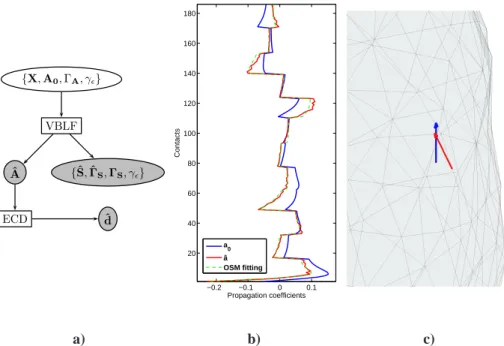
{X, A0, ΓA, γǫ} VBLF ECD {ˆS, ˆΓS, ΓS, γǫ} ˆ A ˆ d −0.2 −0.1 0 0.1 20 40 60 80 100 120 140 160 180 Propagation coefficients Contacts a0 â OSM fitting a) b) c)
Figure 2: a) Work-flow of the method including the ECD identification step, with ˆd the set of identified dipoles. b) Example of a posterior lead-field column mean ˆa (red) superimposed with its OSM fitting (dashed green) and its prior version a0(blue). c) Prior dipole (blue) and fitted dipole (red), 3.1mm distant one from the other in this case (with a prior lead-field resolution of 1cm).
3.1. Simulations
We use the adult MNI-ICBM152 averaged model (Fonov et al. (2011)) which is freely available for download on the web2. The forward model is computed using a five compartment Finite Element Model (FEM) for 509 source positions regularly sampling the gray matter volume. For more details on how the FEM has been computed, please refer to Caune et al. (2014).
To simulate the uncertainties of the forward model, we use One Sphere Models (OSM (Yao (2000))) to solve the inverse problem and build the lead-field prior A0 (with conductivities of 0.33 S/m). M= 17 different OSM are computed using locally
fitted spheres at 17 points3of the upper skull mesh, for which closed-form are avail-able (Zhang (1995)). For each of these 17 models, the lead-field is computed for a regular grid of freely oriented dipoles with 1cm resolution, situated within a 2cm en-velope of the gray matter mesh and with no overlap with the 509 previously sampled positions used form the forward FEM computation (in all, Np= 2214 possible dipole positions). The prior matrix A0and the associated precision matrices{Γai} are then
2http://www.ucl.ac.uk/medphys/research/borl/intro/headmodels/adult
3One on top of the head, 8 around the horizontal plane passing through the nasion, and one at mid-distance of each surface line linking these 8 previous points to the top one
computed using the procedure described section 2.2.1.
We have simulated a realistic SEEG implantation with the help of the neuro-physiologists of the Nancy CHU. The number of electrode shafts equals 12, on which 186 con-tacts are spread (about 14 to 18 per electrodes). Our prior OSM lead-field A0 en-codes the projections in the three directions for each source point, and is then of size
Nc× 3 ∗ Np= 186 × 6642.
Either three or five equivalent dipoles with random positions and orientations are selected among the set of 509 dipoles. We affect real time-courses to these seeded dipoles, taken from the SEEG recordings of an epileptic patient on bipolar montage (difference of two consecutive contacts of a same electrode shaft, assumed to catch the activity of a local source). A set of 200 windows with time-length 256ms (128 samples) have been selected, corresponding to background activities, inter-epileptic events, as well as various representative periods of the ictal events (from spike burst-ing to paroxystic rhythmic activities). Additive spatially independent white noise is simulated on the contacts, with standard deviations taken as:
σε = ||XS||F
T∗ Nc∗ ns∗ 10LSNR/20
(23) with XSthe potential due to the nssimulated sources, and LSNRthe desired SNR in dB which varies in the set{10, 5, 0, −5} in our simulations. The division by nsensure that the SNR for each dipole respectively is comparable on average from a simulation to another across the two source configurations ns= {3, 5}.
We evaluate the benefit of re-estimating the lead-field A by comparing the localiza-tion results based on the proposed VBLF approach (seclocaliza-tion 2.2.2) with a SBL approach (section 2.1). We also compare the performances with SOFOMORE4. While gaussian priors of equal variance are attributed to each projection gain of a given lead-field column in its original version (Stahlhut et al. (2011)), we set the variance values as estimated by our method (i.e., the diagonal values of the covariance matrices as com-puted in equation (9)). SOFOMORE is then a particular case of our approach with diagonal lead-field column precisions. This comparison is carried out to assess the im-portance of explicitly encoding physical model-driven constraints within the lead-field priors. We also compare the results using RAP-MUSIC (Mosher and Leahy (1998)) informed with the true number of sources, and another empirical Bayesian approach called Champagne (Wipf et al. (2010)) for which the true standard-deviation of the noise has been informed. For SBL, RAP-MUSIC, and Champagne, a local OSM lead-field is built: for each position of the lead-lead-field grid, the three cartesian projections are given by the OSM model (among the M= 17 previously computed) whose fitting point
on the skull mesh is the closest to the considered grid point.
3.1.1. Evaluation criteria
The performances of the different algorithms are evaluated based on two comple-mentary metrics. The first one is the Distance of Localization Error (DLE) (Yao and Dewald (2005); Becker et al. (2014)), which measure the localization accuracy of the
true sources while penalizing the presence of spurious sources (false positives). The DLE is given by:
DLE= 1 2nsi
∑
∈S minj∈ ˆS||xi− ˆxj|| + 1 2 ˆns∑
j∈ ˆS mini∈S||xi− ˆxj|| (24)with S and ˆS the set of simulated sources and of estimated sources respectively, xi the position of the ithsimulated source and ˆxjthe position of the jthestimated source, and nsis the number of simulated sources while ˆnsis the number of estimated sources. In this paper, a dipole is included in the solution ˆS if the standard-deviation of its estimated time-course is above a threshold given as the tenth of the largest standard-deviation in the current solution.
The second metric is the A′ metric (Snodgrass and Corwin (1988); Wipf et al. (2010)) which take into account both the ratio of successful source localization (hits) and the ratio of false positives. A simulated source is considered as recovered (true positive) if at least one dipole in the solution ˆS is less than 1cm far from this dipole. The hits rate is the number of true positives divided by the total number of simulated sources ns. Any dipoles in the solution ˆS farther than 1cm from all the true dipoles are considered as false positive. To define a false positive rate, a maximum number of possible false positives has to be defined. This maximum number has been arbitrarily set to 100 in Wipf et al. (2010). In this paper we decide to set it to 48, which is the highest number of false positives obtained in our simulations (Champagne algorithm with 5 dipoles in the−5dB case). Given these hit rates (Hr) and false positives rates
(FPr), the A′metric is computed as (Snodgrass and Corwin (1988)):
A′= (
0.5 + (Hr − FPr)(1 + Hr − FPr)/(4Hr(1 − FPr)), if Hr ≥ FPr
0.5 + (FPr − Hr)(1 + FPr − Hr)/(4FPr(1 − Hr)), if FPr > Hr (25)
In addition, we assess the ability of the methods in estimating the dipoles time-courses and projections on the contacts using the correlation coefficients between the estimations and the ground-truth. Finally, we also evaluate the sparsity of the methods by providing the number of dipoles ˆnsselected in the final solution ˆS.
3.1.2. Results
We iterate 400 simulations for each configuration (number of sources and noise level). For all the algorithm, the variance of the noise is initialized using a minimum description length (MDL) approach (except for RAP-MUSIC where the exact number of sources is given and Champagne to which the true noise variance is given). For all empirical Bayes algorithm, the prior source precisionΓSis set as the identity matrix.
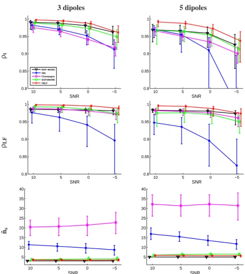
The performances in term of time-course and lead-field reconstructions (fig 3, rows 1 & 2) demonstrate the good performance of our approach. VBLF is indeed consis-tently the most accurate in median over all configurations, with significantly higher time-course correlation rates (ρt) compared to the other methods. The method is par-ticularly accurate in estimating the forward field coefficients, reaching correlation rates
3 dipoles 5 dipoles ρt 10 5 0 −5 0.8 0.85 0.9 0.95 1 SNR RAP−MUSIC SBL Champagne SOFOMORE VBLF 10 5 0 −5 0.8 0.85 0.9 0.95 1 SNR ρLF 10 5 0 −5 0.8 0.85 0.9 0.95 1 SNR 10 5 0 −5 0.8 0.85 0.9 0.95 1 SNR ˆns 10 5 0 −5 5 10 15 20 25 30 35 40 SNR 10 5 0 −5 5 10 15 20 25 30 35 40 SNR
Figure 3: Performance evaluation for 3 (first column) and 5 (second column) simultaneous dipoles. Medians of the correlation coefficients of the estimated time-course and lead-field projections with the ground-truth are given on resp. first (ρt) and second (ρLF) rows. The median number of significant dipoles in the solution
( ˆns) for each method are given on the third row. Error bars corresponding to first and third quartiles are also
given.
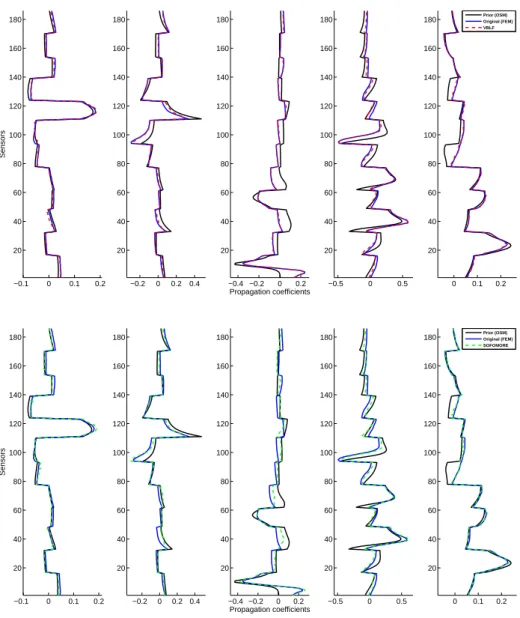
ρLF over 0.99 for 3 and 5 dipoles form 10 to 0dB SNR. If SOFOMORE manages to compete with both RAP-MUSIC and Champagne in the 3 dipoles case, it is less accu-rate than these two fixed lead-field methods in reconstructing the lead-field columns in the 5 dipoles case. This proves that it might be inappropriate to give degrees of freedom to the lead-field coefficients if the optimization procedure is not carefully constrained. On fig.4 are given an example of lead-field coefficients re-estimates (i.e., including the post-ECD scaling procedure) for both VBLF and SOFOMORE, for the 5 dipoles/10dB simulation case. Starting with an OSM prior, VBLF proves to be able to produce
rel-evant forward field posterior mean close to the true (simulated) one, here given by a FEM. The unconstrained version (i.e., SOFOMORE, diagonal precision matrix over the columns of A) brings less accurate estimates (see fig.4, 2ndrow 3rdcolumn in par-ticular, errors are visible between the blue and dashed green lines). Such bad estimates interfere with the estimates of the other simultaneous dipoles, impacting significantly the localization results.
One can notice the good performance of the Champagne algorithm in this recon-struction task, this method being originally dedicated to robust estimation of the source time-courses (Wipf et al. (2010)). RAP-MUSIC also manage to produce reliable esti-mates of the lead-field and time-courses, the method is successful in identifying the 3D subspaces best fitting the projections of each simulated dipole.
The performances of both SOFOMORE and VBLF in estimating the true number of sources are consistently very near the RAP-MUSIC reference (true number of sources informed), with a small but significant advantage for our VBLF approach considering the tight quartile values (see the ˆnsmetric, third row of fig 3). These methods are able to retrieve the true number of sources even in case of strong interferences (up to 5 simultaneous dipoles) and noise level (-5dB on average for each dipole), while Cham-pagne and SBL provides large over-estimations of the number of underlying sources. This can be explained by the basis mismatch issue as discussed in (Chi et al. (2011)), the true forward field of the sources being not perfectly aligned with any columns of the lead-field matrix, a high number of lead-field elements are necessary for the algo-rithm to reconstruct the observations. The re-estimation of these lead-field columns in SOFOMORE or VBLF brings a data-driven fitting of the lead-field to the true source projection, avoiding such scattering effects.
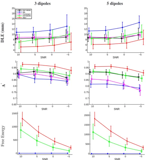
The performances in term of localization precision (DLE) and A’ metric are given fig 5. The informed version of RAP-MUSIC is expected to provide accurate results in this context of additive white Gaussian noise. The Champagne approach also provides very accurate localization results, with DLE below or very near to 1cm within each ns and SNR configurations. However as shown by the rather high number of significantly powerful sources in the solution (see fig 5), the number of false positives can be high as shown by the A′metric, especially in the ns= 5 dipoles case.
After applying the ECD fitting step (as described section 2.2.3), VBLF brings the best DLE performance, in concordance with the high accuracy of the source lead-field estimates. The DLE is decreased of about 2mm in median with respect to SOFOMORE over all configurations, which can be considered as a significant gain in accuracy con-sidering that the DLE are consistently below 1cm (representing roughly a gain in per-formance of about 20%). The true number of sources being accurately estimated by VBLF, very few false positives are produced, explaining the high A’ values. This is not observed for SOFOMORE, for which the rather low number of false positives are compensate by higher localization errors due to inaccuracies in the source lead-field estimates. The superiority of our method with respect to the SOFOMORE approach demonstrates the importance of constraining the dipole projections through the intro-duction of non-null off-diagonal values in eachΓai.
A last metric is given by the final values of the free energy function (equation (21)) which describe the relevance of the model to the data (Friston et al. (2008)). This lower bound of the model evidence can be evaluated for SBL, SOFOMORE and VBLF. While
−0.1 0 0.1 0.2 20 40 60 80 100 120 140 160 180 Sensors −0.2 0 0.2 0.4 20 40 60 80 100 120 140 160 180 −0.4 −0.2 0 0.2 20 40 60 80 100 120 140 160 180 Propagation coefficients −0.5 0 0.5 20 40 60 80 100 120 140 160 180 0 0.1 0.2 20 40 60 80 100 120 140 160
180 Prior (OSM)Original (FEM) VBLF −0.1 0 0.1 0.2 20 40 60 80 100 120 140 160 180 Sensors −0.2 0 0.2 0.4 20 40 60 80 100 120 140 160 180 −0.4 −0.2 0 0.2 20 40 60 80 100 120 140 160 180 Propagation coefficients −0.5 0 0.5 20 40 60 80 100 120 140 160 180 0 0.1 0.2 20 40 60 80 100 120 140 160
180 Prior (OSM)Original (FEM) SOFOMORE
Figure 4: An illustration of the lead-field coefficients estimates when using VBLF (top/dashed red) or SO-FOMORE (bottom/dashed green), in the 5 dipoles case - 10dB (one figure per dipole). The estimates are super-imposed with the true FEM lead-field (blue) and the prior column (black).
the actual values of this function has no meaning in itself, its comparison from a model to another can be used to determined which model is the most appropriate to explain the data (fixed lead-field (SBL), diagonal lead-field column covariance matrices (SOFO-MORE), and non-diagonal lead-field column covariance matrices (VBLF)). Using the values of the SBL free energy estimates as a reference (setting it to 0), VBLF provides
3 dipoles 5 dipoles D L E (m m ) 10 5 0 −5 4 6 8 10 12 14 16 18 20 SNR RAP−MUSIC SBL Champagne SOFOMORE VBLF 10 5 0 −5 4 6 8 10 12 14 16 18 20 SNR A ′ 10 5 0 −5 0.65 0.7 0.75 0.8 0.85 0.9 0.95 1 SNR 10 5 0 −5 0.65 0.7 0.75 0.8 0.85 0.9 0.95 1 SNR F re e E n er g y 10 5 0 −5 0 500 1000 1500 SNR 10 5 0 −5 0 500 1000 1500 2000 SNR
Figure 5: Performance evaluation for 3 (first column) and 5 (second column) simultaneous dipoles. Median of the DLE and A′metrics are given resp. on the first and second rows. On the third row is given the relative median values of the Free Energy for VBLF and SOFOMORE with respect to the SBL reference values. Error bars of first and third quartiles are superimposed.
the highest free energy values over all the configuration and confirms its relevance for this simulated source localization task (bottom figures of fig 3).
3.2. Intracranial Stimulations
The localization method is tested on Intracranial Stimulation (ICS) data, where two consecutive electrode contacts are used to inject a current in the brain volume. We will consider a data set from a 40-year-old man with presumed bitemporal lobe epilepsy. He was implanted with ten depth electrodes in the right temporal lobe and insular cortex
0 1 T’5 T’4 T’3 T’2 T’1 B’13 B’12 B’11 B’10 B’ 4 B’ 3 B’ 2 B’ 1 A’13 A’12 A’ 5 A’ 4 A’ 3 A’ 2 A’ 1
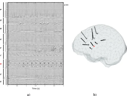
Figure 6: One second of SEEG signals recorded during an ICS session on TB’8-9. These 20 channels are used for the localization of the stimulation.
and four in the left temporal lobe. The reference was FPz surface electrode from the classical 10-20 system. The depth contacts coordinates were automatically determined using the procedure described in Hofmanis et al. (2011). We consider stimulations injected in the left (less implanted) hemisphere, using the contacts of the electrodes TB’.
Three ICS data-set are used, and correspond to a profound (TB’2-3), intermediate (TB’4-5) and superficial (TB’8-9) stimulation site. The stimulation is applied for about 4s for each site, and consists it in a train of 55 biphasic pulses/s. We have extracted 3s of signal centered within the stimulation window, and we cut it in 12 sub-windows of 250ms each (thus 13 to 14 pulses per window). The localization is applied separately on each sub-windows. While it is true that the ICS source is stronger than physiolog-ical sources, it may not be the dominant activity recorded by far electrodes on which local physiological activities are super-imposed. On figure 6, the time-courses of the potentials generated by the ICS dipoles for the stimulation site TB’8-9 are given. On the contact T’1, distant of 36mm from the stimulation site, the potentials due to the ICS source are visible but is clearly weaker than the surrounding physiological activity.
The lead-field matrix is built based on 17 locally fitted OSM using a 1cm resolu-tion grid (like in the simularesolu-tions), the spheres being fitted on 17 well distributed points on the upper part of the inner skull. The contacts of the electrode TB’ used for the stimulation are not considered. We aim at localizing the stimulation based only on a limited set of distant contacts. We restrict the used measurements to those of the hemi-sphere of the stimulation, thus 20 channels spread on 3 electrode shafts (A’,B’,T’, see fig 6). Using electrode shafts can pose a conditioning problem, as tackled in previous works (Caune et al. (2014)). We arrived to the conclusion that at least a dozen contacts from 3 different electrode shafts are needed to successfully carry out a brain source localization, such conditions being met in the particular case of this data set.
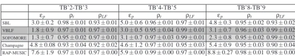
The position errorsεpare given in table 1, averaged over the 12 sub-windows local-ization results. After convergence, each algorithm generates solutions whose powers
TB’2-TB’3 TB’4-TB’5 TB’8-TB’9 εp ρt ρLF εp ρt ρLF εp ρt ρLF SBL 3.0 ± 0.2 0.98 ± 0.01 0.93 ± 0.01 5.0 ± 0.6 0.96 ± 0.01 0.97 ± 0.01 4.8 ± 0.3 0.95 ± 0.02 0.93 ± 0.02 VBLF 1.8 ± 0.9 0.97 ± 0.01 0.97 ± 0.01 3.0 ± 0.5 0.95 ± 0.04 0.99 ± 0.01 3.1 ± 0.7 0.96 ± 0.03 0.99 ± 0.02 SOFOMORE 1.3 ± 0.7 0.95 ± 0.02 0.97 ± 0.01 3.1 ± 0.7 0.97 ± 0.03 0.99 ± 0.01 2.3 ± 0.8 0.95 ± 0.02 0.99 ± 0.02 Champagne 4.8 ± 0.08 0.93 ± 0.04 0.92 ± 0.02 4.6 ± 1.2 0.97 ± 0.01 0.95 ± 0.03 5.4 ± 0.9 0.95 ± 0.03 0.90 ± 0.04 RAP-MUSIC 7.6 ± 1.9 0.97 ± 0.01 0.97 ± 0.00 5.9 ± 0.0 0.99 ± 0.00 0.97 ± 0.00 8.8 ± 0.27 0.98 ± 0.01 0.98 ± 0.00
Table 1: Performance values for the localization of three ICS dipoles (averaged over 12 windows of 250ms each) for five different algorithms: SBL, VBLF, SOFOMORE, Champagne and RAP-MUSIC. Position er-rorsεp are given in mm. Correlation coefficientsρt between the mean of the closest (<1cm) significant
source time-courses and the potential recorded on the electrode of stimulation next to the stimulated con-tacts. Correlation coefficientsρLFbetween the mean lead-field projections of the closest significant sources
(re-estimated in the case of VBLF and SOFOMORE) and an estimation of the true projection of the dipole of stimulation based on the One Sphere Model.
are concentrated around the position of the stimulation dipole. We retain the time-course and lead-field projection of the equivalent dipole of maximum power as this representing the stimulation dipole. In the table 1 are then given two additional perfor-mance values (averaged over the 12 sub-windows): ρt is the correlation coefficient between the estimated equivalent dipole time course and the potential recorded on a non-saturated (manually chosen) contact belonging to the electrode of stimulation.
ρLF is the correlation coefficient between the estimated equivalent dipole lead-field projection with an OSM estimated projection of the dipole of stimulation using its true position and orientation.
The performances of all five algorithms (SBL, VBLF, SOFOMORE, Champagne as well as RAP-MUSIC) are evaluated (considering the post-optimization of section 2.2.3 for both SOFOMORE and VBLF). The number of sources in RAP-MUSIC has been informed through an MDL approach (1 to 3 sources are estimated depending on the analyzed window). All algorithms are successful in localizing the stimulation dipole (under 1cm on average with small standard-deviation), with consistent advantages for SBL and SOFOMORE for which the regressed dipole is about 2 to 3 mm from the stimulation site (taken as the middle of the two stimulated contacts). These results are competing with the localization using an ECD approach applied on the averaged stimulation peaks within a window of 2.5s (see Caune et al. (2014)). This can be taken
as proofs that (i) the lead-field projection is indeed well recovered (further confirmed by theρLF correlation values) and (ii) the OSM indeed provides a reliable approximation of the head propagation medium when a precision of the order of few millimeters is needed. Relying on recent studies on the topic (Birot et al. (2014); Caune et al. (2014)), OSM is reported to provide a reliable approximation of the real propagation medium and is accurate enough to reach precise localization errors of the order of few millimeters, especially in this context of intracranial SEEG recordings where we are far less impacted by errors in the skull:brain ratio estimate than in the case of scalp recordings (Acar and Makeig (2013); Acar et al. (2016)).
3.3. Epileptic interictal spikes
We now evaluate the methods on a data set of interictal spikes recorded from a 28 year-old woman with drug-resistant insulo-opercular epilepsy (already included in a
0 0.5 1 1.5 2 2.5 3 S’6 S’5 S’4 S’3 S’2 S’1 C’ 12 C’ 11 C’ 10 C’ 9 C’ 8 C’ 7 C’ 6 C’ 5 C’ 4 C’ 3 C’ 2 C’ 1 R’10 R’9 R’8 R’7 R’6 R’5 R’4 R’3 R’2 R’1 L’8 L’7 L’6 L’5 L’4 L’3 L’2 L’1 F’ 8 F’ 7 F’ 6 F’ 5 F’ 4 F’ 3 F’ 2 F’ 1 X’12 X’11 X’10 X’9 X’8 X’7 X’6 X’5 X’4 X’3 X’2 X’1 B’ 10 B’ 9 B’ 8 B’ 7 B’ 6 B’ 5 B’ 4 B’ 3 B’ 2 B’ 1 T’7 T’6 T’5 T’4 T’3 T’2 T’1 P’18 P’17 P’16 P’15 P’14 P’13 P’12 P’11 P’9 P’8 P’7 P’6 P’5 P’4 P’3 P’2 P’1 Time (s) T’ B’ T’ X’ F’ L’ R’ C’ 1mv P’ S’ a) b)
Figure 7: a) SEEG signals of interictal spikes in common reference montage (FPz scalp electrode). Epileptic spikes are maximally visible on the contacts 5 and 6 of the depth electrode R’ (left central operculum). b) Mesh of the head and SEEG configurations. The labels are near the most profound contact of their corresponding electrode shaft, i.e., the contact 1.
previous paper (Caune et al. (2014))). She gave her informed consent prior to partici-pation. The intracranial EEG (SEEG) recording setup consists in ten electrode shafts implanted in the insulo-opercular regions (internal and lateral contacts, see fig.7(b)): P’, cingulum/parietal operculum ; T’, infero-anterior insula/ superior temporal gyrus ; B’, anterior insula/pre-motor cortex; X’, posterior insula/post-central gyrus; F’, and L’, anterior and posterior part of the inferior frontal sulcus/middle frontal gyrus; R’, middle insula/central operculum; C’, cingulum/middle frontal gyrus; S’, superior frontal sul-cus; M’, supplementary motor area/superior frontal gyrus. The inspection of the SEEG data on bipolar montage reveals the presence of interictal epileptic spikes near the R’ depth electrode, especially on the contacts R’5 and R’6, which also impact neighboring electrodes (especially T’ and X’), though with rather low signal to noise ratios. Within the time windows of spikes occurrence (about 100ms length), few other activities of lower amplitudes are impacting the electrodes. We then expect to localize the main generator(s) within a focal area surrounding the electrode shaft R’. Three seconds of interictal recordings on the 100 available contacts are given fig. 7(a).
Several OSM are computed to build the lead-field matrix used for the inversion. 17 local spheres are fitted on the inner skull of the patient following the procedure described above, and we use a regular 3D grid with 7mm resolution restricted to the
implanted hemisphere for the forward model computation, yielding 2322 source po-sitions (i.e., 6966 columns in the forward matrix A). The coordinates of the depth contacts were obtained as for the ICS localization described above. All the contacts, at the exception of those of the electrode R’, are used to perform the localization, i.e., 90 recording channels.
The bipolar analysis of the R’ shaft reveals a polarity inversion between R’6 and R’7, indicating a dipolar source situated in a plane between the two contacts and having a strong component oriented orthogonal to this plane. From the potential time course recorded on the contact R’6, 20 interictal spikes have been identified through a simple thresholding process and validated by the expert. The localization is carried out after averaging the 20 time windows of 64 samples (125ms), thus enhancing the signal to noise ratio of the inter-ictal activity of interest.
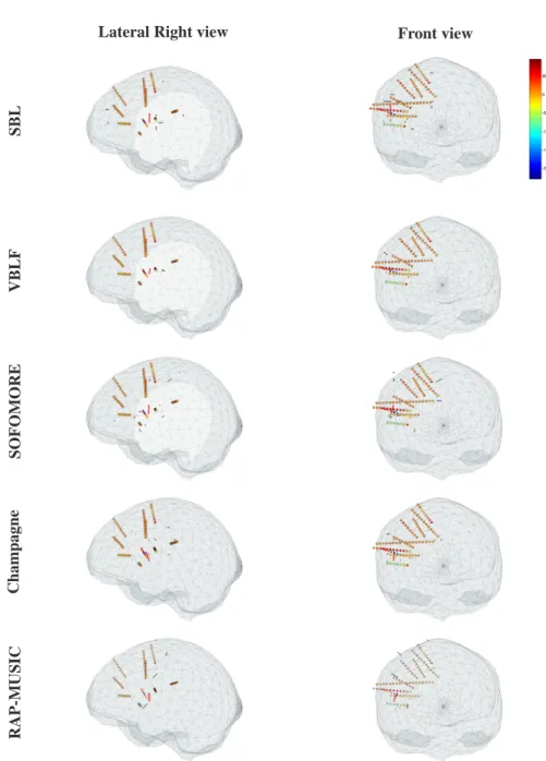
The same five algorithms were tested on this data set. Again, MDL is used for the initialization of RAP-MUSIC (resulting in 7 estimated sources). Figure 8 illustrates the localization map for each tested algorithm. The localization of the most intense equivalent dipole is concordant for all the methods, distant from 6.2mm to 9.8mm from
the R’6 contact, and with a maximum distance of 6mm between the two most distant solutions (SBL with RAP-MUSIC). It is also consistent with the localization results obtained using an ECD approach in a recent paper (Caune et al. (2014)), and validated by the expert.
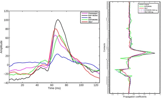
In particular, the localization map is very sparse for the VBLF approach, five co-ativated dipoles (i.e., with a standard deviation over the tenth of the most intense dipole) are found within the cloud of the electrodes, explaining co-occuring activities of low amplitudes. These dipoles are localized within the boundaries of the brain (gray matter) mesh. Champagne also provide a similarly sparse localization map, although yielding nine co-occuring equivalent dipoles. SOFOMORE as well as SBL are providing less sparse maps. Both approaches are estimating dipoles of relative high intensity and distant from the cloud of electrodes (out of the brain mesh in some case), while such results seem to be irrelevant for this given data for which the main activities are clin-ically presumed to take place near the electrode R’. Finally, VBLF and Champagne are producing very similar time courses for the main equivalent dipole, having their maximum peak at the same instant, while the activities estimated by the three other algorithms are delayed of a few samples (fig. 9 left).
When comparing the estimated lead-field projection given by the VBLF and the SOFOMORE approach (fig. 9 right), one can see the somewhat unplausible estimate of the lead-field projection produced by SOFOMORE, while the estimate of the VBLF approach is more relevant. This is confirmed when applying the fitting of both esti-mated columns using the OSM. The resulting mean squared error of the OSM fitting is of 0.01 for the VBLF estimate while it reaches 0.08 in the case of SOFOMORE.
4. Discussion
In this study we propose a distributed approach for simultaneous estimation of the brain source activities under controlled re-adjustment of their lead-field projections A, based on a Variational Bayesian (VB) scheme. The re-estimation of the columns are
Lateral Right view Front view S B L V B L F S O F O MO R E C h a m p a g n e R A P -MU S IC
Figure 8: Localization maps of averaged inter-ictal spikes (20 events) over a window length of 125ms (64 samples), centered on the maximum values of each spike (as recorded on the electrode R’6). The potential values (µV ) on the electrodes are given as colors (dark blue for negative values to dark red for positive values, see colorbar), and the contacts used for the localization are black circled (all electrodes except R’ on which the interictal spikes has been identified by the expert). Two views (lateral right and frontal) are given. The dipoles in red represent the equivalent dipoles identified as the estimated generators of the interictal spikes, while the dipoles in black represent the simultaneous activities estimated by each algorithm.
20 40 60 80 100 120 −40 −20 0 20 40 60 80 100 120 Time (ms) Amplitude Champagne RAP−MUSIC SBL SOFOMORE VBLF −1.5 −1 −0.5 0 0.5 1 1.5 2 2.5 3 P’1 P’2 P’3 P’4 P’5 P’6 P’7 P’8 P’9 P’11 P’12 P’13 P’14 P’15 P’16 P’17 P’18T’1 T’2 T’3 T’4 T’5 T’6 T’7 B’ 1 B’ 2 B’ 3 B’ 4 B’ 5 B’ 6 B’ 7 B’ 8 B’ 9 B’ 10X’1 X’2 X’3 X’4 X’5 X’6 X’7 X’8 X’9 X’10 X’11 X’12F’ 1 F’ 2 F’ 3 F’ 4 F’ 5 F’ 6 F’ 7 F’ 8L’1 L’2 L’3 L’4 L’5 L’6 L’7 L’8 C’ 1 C’ 2 C’ 3 C’ 4 C’ 5 C’ 6 C’ 7 C’ 8 C’ 9 C’ 10 C’ 11 C’ 12S’1 S’2 S’3 S’4 S’5 S’6 S’7 S’8 M’ 1 M’ 2 M’ 3 M’ 4 M’ 5 M’ 6 M’ 7 M’ 8 Propagation coefficients Contacts Original SOFOMORE VBLF SOFOMORE OSM reg. VBLF OSM reg.
Figure 9: Left: estimated time courses for the equivalent dipoles of maximum power for each algorithm. Right: original projection coefficients on the 90 contacts for the elementary dipole chosen by both VBLF and SOFOMORE, along with the lead-field optimization given by each algorithm, on which are super-imposed their OSM regressions (dashed lines).
controlled through covariance matrices, constraining the projections to remain physi-ologically plausible, i.e., preventing to deviate implausibly from prior projection pat-terns A0computed using a physical propagation model. We provide comparisons with several algorithms from the literature (SBL, SOFOMORE, Champagne, RAP-MUSIC) with several noise level configurations, giving quantitative facts on the benefits of tak-ing account of the forward model uncertainties.
The simultaneous optimization of the source time-courses and of the lead-field pro-jections implies that the estimated lead-field columns ˆA do not corresponds anymore
with the projection of unitary dipolar elements as initially encoded in A0, in term of positions, orientations and (unitary) amplitudes. The ambiguity in the estimated source parameters can be disentangled by a fitting of the posterior columns based on an ana-lytical model, such as the One Sphere model used in this study. In this perspective, the VBLF approach can be seen as a decomposition on a continuous dictionary where the dictionary atoms are iteratively learned from the observations (Yang et al. (2013)). The method separates the different sources contributing to the data, and optimizes their pro-jection gains on the contacts through a constrained data-driven procedure. The modi-fied projection gains are then mapped and scaled to their corresponding unitary dipolar components in the source space through a classical Scherg’s single-dipole inversion, providing the final source parameter estimates.
While this is a distributed approach in its formulation, our methods might be seen as an ECD approach where thousands of dipole candidates are simultaneously
opti-mized in their amplitudes, positions and orientations. This preclude the initialization issues (multi-start strategies, initial guess of the number of dipoles) encountered when dealing with the ECD approaches (Scherg et al. (1999); Kiebel et al. (2008); Caune et al. (2014)).
The gain in sparsity is significant when the lead-field is reconsidered (both for SOFOMORE and our method), and the size of the estimated source space is con-sistently very close to the true one in the simulated case. By offering such flexible framework, both the estimation of the equivalent dipoles projections and time-courses are enhanced, on condition that the correction of the projection coefficients is care-fully controlled. Indeed the unconstrained re-evaluation scheme (i.e., SOFOMORE) leads globally to less accurate estimation results than our constrained version (VBLF), especially for low SNR levels.
Our approach provides consistent results when applied on real data. First, its appli-cation to an Intracranial Stimulation (ICS) data set demonstrates its ability to provide accurate localization, time course estimation and lead-field projection estimates in a real context. Secondly, the method proves to produce plausible localization map in a case of inter-epileptic spikes localization. The result is concordant with the expertise of the neurologists. In this last case, the importance of using non-diagonal covari-ance matrix for modeling the lead-field column distribution is further illustrated, as the lead-field estimate produce by SOFOMORE is not physiologically relevant.
It is worth noticing that the localization accuracy could obviously be enhanced by introducing a finer grid of elementary dipole positions. However it would still remains a discrete sampling of the source space with uncertain model projections, thus prone to mismatch basis issues (Chi et al. (2011)). Also, it would result to a higher compu-tational burden. To give a quantitative comparison, in the simulated case our VBLF scheme takes about 2 minutes for 1000 iterations with the considered lead-field grid of 1cm resolution (6642 columns), while the SBL approach takes about 1 minute for the same number of iterations. Besides, the variational Bayesian optimization scheme is reported to be slow. As a faster alternative, modified versions of the gradient descent al-gorithms inspired from MacKay (1992); Miele and Cantrell (1969); Zheng et al. (2015) could be adopted, through a direct gradient optimization of the free-energy function.
The analysis of the confidence we can place in a localization result must be deep-ened, in particular in this difficult context of SEEG recordings where the conditioning of the electrode shafts and their positions with regard to the structures of interest are sensitive questions. Such issues have been tackled in a previous study (Caune et al. (2014)) in the case where a single dominant dipole is to be identified, based on a dipole fitting (ECD) procedure. The case of multiple simultaneous sources can now be studied through the use of the proposed distributed source models, with the aim to provide a clinical added value on how the electrode shafts has to be implanted for reaching confident localization results covering the whole brain volume, or at least for the brain structures suspected to contain the sources of interest. In this perspective, extended validation campaign on real recordings of interictal spikes, or more likely on evoked potential activities (for which the source positions, time courses and instant of apparition are perfectly controlled), must be carried out in close collaboration with neurophysiologists.
5. Acknowledgments
The authors thank Prof. S. Colnat-Coulbois (Nancy) for the neurosurgical contri-butions, and the project ANR SEPICOT for their financial support.
6. References
Acar, Z. A., Acar, C. E., Makeig, S., 2016. Simultaneous head tissue conductivity and EEG source location estimation. NeuroImage 124, 168–180.
Acar, Z. A., Makeig, S., 2013. Effects of forward model errors on eeg source localiza-tion. Brain topography 26 (3), 378–396.
Baillet, S., Mosher, J. C., Leahy, R. M., 2001. Electromagnetic brain mapping. Signal Processing Magazine, IEEE 18 (6), 14–30.
Bangera, N. B., Schomer, D. L., Dehghani, N., Ulbert, I., Cash, S., Papavasiliou, S., Eisenberg, S. R., Dale, A. M., Halgren, E., 2010. Experimental validation of the influence of white matter anisotropy on the intracranial eeg forward solution. Journal of computational neuroscience 29 (3), 371–387.
Becker, H., Albera, L., Comon, P., Gribonval, R., Wendling, F., Merlet, I., 2014. A per-formance study of various brain source imaging approaches. In: Acoustics, Speech and Signal Processing (ICASSP), 2014 IEEE International Conference on. IEEE, pp. 5869–5873.
Birot, G., Spinelli, L., Vulliémoz, S., Mégevand, P., Brunet, D., Seeck, M., Michel, C. M., 2014. Head model and electrical source imaging: a study of 38 epileptic patients. NeuroImage: Clinical 5, 77–83.
Bishop, C. M., et al., 2006. Pattern recognition and machine learning. Vol. 1. springer New York.
Caune, V., Le Cam, S., Ranta, R., Maillard, L., Louis-Dorr, V., 2013. Dipolar source localization from intracerebral SEEG recordings. In: Engineering in Medicine and Biology Society (EMBC), 2013 35th Annual International Conference of the IEEE. IEEE, pp. 41–44.
Caune, V., Ranta, R., Le Cam, S., Hofmanis, J., Maillard, L., Koessler, L., Louis-Dorr, V., 2014. Evaluating dipolar source localization feasibility from intracerebral SEEG recordings. NeuroImage 98, 118–133.
Chang, N., Gulrajani, R., Gotman, J., 2005. Dipole localization using simulated intrac-erebral EEG. Clinical neurophysiology 116 (11), 2707–2716.
Chi, Y., Scharf, L. L., Pezeshki, A., Calderbank, A. R., 2011. Sensitivity to basis mismatch in compressed sensing. Signal Processing, IEEE Transactions on 59 (5), 2182–2195.