HAL Id: hal-01879384
https://hal.laas.fr/hal-01879384
Submitted on 23 Sep 2018
HAL is a multi-disciplinary open access
archive for the deposit and dissemination of
sci-entific research documents, whether they are
pub-lished or not. The documents may come from
teaching and research institutions in France or
abroad, or from public or private research centers.
L’archive ouverte pluridisciplinaire HAL, est
destinée au dépôt et à la diffusion de documents
scientifiques de niveau recherche, publiés ou non,
émanant des établissements d’enseignement et de
recherche français ou étrangers, des laboratoires
publics ou privés.
Multi-Agent Cooperative Load Manipulation
Antonio Franchi, Antonio Petitti, Alessandro Rizzo
To cite this version:
Antonio Franchi, Antonio Petitti, Alessandro Rizzo. Distributed Estimation of State and Parameters
in Multi-Agent Cooperative Load Manipulation. IEEE Transactions on Control of Network Systems,
IEEE, 2018, �10.1109/TCNS.2018.2873153�. �hal-01879384�
Distributed Estimation of State and Parameters in
Multi-Agent Cooperative Load Manipulation
Antonio Franchi, Senior Member, IEEE, Antonio Petitti, Alessandro Rizzo, Senior Member, IEEE
Abstract—We present two distributed methods for the estima-tion of the kinematic parameters, the dynamic parameters, and the kinematic state of an unknown planar body manipulated by a decentralized multi-agent system. The proposed approaches rely on the rigid body kinematics and dynamics, on nonlinear observation theory, and on consensus algorithms. The only three requirements are that each agent can exert a 2D wrench on the load, it can measure the velocity of its contact point, and that the communication graph is connected. Both theoretical nonlinear observability analysis and convergence proofs are provided. The first method assumes constant parameters while the second one can deal with time-varying parameters and can be applied in parallel to any task-oriented control law. For the cases in which a control law is not provided, we propose a distributed and safe control strategy satisfying the observability condition. The effectiveness and robustness of the estimation strategy is showcased by means of realistic MonteCarlo simulations.
I. INTRODUCTION
In this paper, we propose what we believe is the first fully-distributed method for the estimation of all the quantities and parameters needed by a planar robotic multi-agent system to collectively manipulate an unknown load. In particular, the proposed algorithm provides the estimation of the kinematic parameters (equivalent to the grasp matrix), the dynamic parameters (relative position of the center of mass, mass, and rotational inertia) and the kinematic state of the load (velocity of the center of mass and rotational rate).
Most of the works on cooperative manipulation in the liter-ature assume the a priori knowledge of the inertial parameters of the load, even though this assumption does not always hold in real-world scenarios [1]–[5]. Collective manipulation tasks would benefit from the implementation of on-line estimation strategies of inertial parameters of unknown loads for at least two reasons: first, existing control strategies, such as force control and pose estimation, could be effectively applied with satisfactory performance and a reduced control effort. Second, time-varying loads could be effectively manipulated, toward the implementation of adaptive or event-driven control strategies in uncertain environments. Furthermore, similarly to
A. Franchi is with CNRS, LAAS, 7 avenue du colonel Roche, F-31400 Toulouse, France and Univ de Toulouse, LAAS, F-31400 Toulouse, France
A. Petitti is with the Institute of Intelligent Industrial Technologies and Systems for Advanced Manufacturing, National Research Council (STIIMA-CNR), 70126 Bari, Italy,[email protected]
A. Rizzo is with the Dipartimento di Elettronica e Telecomunicazioni, Politecnico di Torino, Corso Duca degli Abruzzi 24, 10129 Torino, Italy
This research was partially supported by the ANR, Project ANR-17-CE33-0007 MuRoPhen, by the Siebel Energy Institute, and by Compagnia di San Paolo.
other applications in multi-agent systems, a distributed and de-centralized implementation of such estimation strategies would provide robustness and scalability. Research on the estimation of inertial parameters is at its early stage, and main limitations of the existing approaches reside in their centralization and in the use of absolute position and acceleration measurements, which are hard and costly to achieve, especially if accurate and noise-free information is needed. Moreover, centralized strategies are notoriously poorly scalable and not robust, due to the existence of single points of failure [6]–[9].
In this paper we propose two algorithms that have instead the following characteristics: (i) there is no central processing unit; (ii) each agent is only able to exchange information with its neighbors in the communication network; (iii) the network, modeled as an undirected graph, can have any topology, provided that it is connected; (iv) each agent is able only to perform local sensing and computation; and (v) the amount of memory and number of computations per step needed by each local instance of the algorithm do not depend on the number of agents but only on the number of communication neighbors. The only assumptions needed are that each agent is able to apply a wrench to the load at its contact point and to measure the velocity of such contact point. Any other measure-ment (such as, e.g., position, distance, acceleration, and gyro measurements) is not available to the agents. Finally, nothing is known about the manipulated load. The approaches are totally distributed, and rely on the geometry of the rigid body kinematics, the rigid body dynamics, on nonlinear observation theory, and on consensus strategies.
Related works: In [10], a decentralized motion control approach based on force consensus, which does not rely on explicit communication among the agents, is proposed. However, the result is achieved at the expense of assuming the presence of a leader agent that steers the load and on an even number of agents arranged in a particular shape called by the authors ‘centrosymmetric’. On the contrary, here we assume that agents can actually communicate, yet we do not assume the presence of a leader and we allow for any unknown spatial arrangement of the contact points. A communication-less adaptive motion control strategy is proposed in [11], under the assumption of a centralized measurement of the center of mass velocity and the load angular velocity. In the methods proposed here, no centralized measurement is needed. Furthermore, differently from [10], [11] our two methods let each agent estimate all the parameters of the problem, thus paving the way for the utilization of any control task (e.g., motion control, force control, etc.) on top of the pro-posed estimation algorithm. The authors in [12] show how a ‘communication-less’ parameter estimation can be achieved by
contact point (CP) wrench applied to the CP
CP velocity communication link
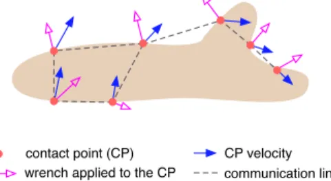
Fig. 1: Conceptual representation of a group of n agents manipulating an object on a plane. The orange dots represent the contact points of each agent, each blue arrow is the velocity of the contact point measured by each agent and each magenta hollow arrow is the wrench (force and torque) applied by each agent at the corresponding contact point. Dashed lines represent the communication links between agents, which all together constitute the communication graph.
adding some stronger assumptions. The method assumes initial parallel execution of synchronized control sequences by all the agents, which requires a form of centralization, prevents the simultaneous estimation of the parameters while performing the control task, and is not suited to estimate time-varying parameters. In our two methods, a-priori synchronization is not required, and the second method (see Sec. VI) can estimate time-varying parameters while performing any control task. The method in [12] assumes also that the robot are localized in position and orientation on a common frame and that they have enough strength to perform a hybrid position/force control and to lift the load from the ground, exploiting the gravity to estimate the mass. Such assumptions are absent in our setting. In fact, our main contribution is to demonstrate that if communication is available then it is possible to solve the estimation in a fully distributed way with minimal sensing.
II. MODEL ANDPROBLEMSTATEMENT
In this section, we formally define the problem of dis-tributively estimating all the parameters and the time-varying quantities that are present in the mechanical model of a team of n planar robotic agents that cooperatively manipulate an unknown planar load, as illustrated in Fig. 1. We assume n to be constant and known to all robots. This assumption can be easily relaxed by implementing one of the several algorithms for the distributed estimation of a graph size [13].
We denote the inertial frame with W = O xy and the load body frame with B = C xByB, where C is the
center of mass (CoM) of the unknown body, indicated with B. We indicate with pC 2 R2 and vC = ˙pC the position
and velocity of C expressed in W, respectively, and with ! 2 R the intensity of the load angular velocity, hereafter called simply angular rate. The dynamics of the manipulated load is described by the rigid body dynamical equation
M ˙⌫ + g = u, (1)
where ⌫ = (v>
C !)> 2 R3 is the twist of B; M =
diag(m, m, J) 2 R3⇥3 is the inertia matrix with m > 0
and J > 0 being the mass and the rotational inertia of the load, respectively; g 2 R3 is the wrench resulting from the
environmental forces such as friction or gravitation. Without
loss of generality, in this work we set g = 0. This is equivalent to assume a horizontal workspace and a wheeled load, for which the friction effects are negligible [14]. Finally, u 2 R3
denotes the external wrench applied by the agents to B, which will be characterized in the following. All the previous quantities are expressed with respect to the frame W.
Each agent i contributes to the overall manipulation by exerting a wrench ui= (fi>⌧i)>2 R3, expressed in W, with
i = 1 . . . n. The force fi2 R2is applied by agent i to a contact
point Ciof B, and ⌧i 2 R is the intensity of the torque applied
about the normal direction to the plane xy. We assume that contact points do not overlap, i.e., Ci 6= Cj, 8i, j = 1 . . . n.
The total external wrench applied to B is u =Pn
i=1Giui=
G¯u, where Gi2 R3⇥3is the partial grasp matrix, G 2 R3⇥3n
is the grasp matrix, and ¯u = u1>, . . . , un> >is the stacked
applied wrench vector that groups the generalized contact force components transmitted through the contact points [15]. The partial grasp matrix is defined as Gi = PiR¯i, where
Pi =
h I2⇥2 02⇥1
[(pCi pC)?]> 1
i
and ¯Ri = I3⇥3, in our setting,
for all i = 1 . . . n. Here, pCi 2 R
2 is the position of C i in
W. The operator (·)? rotates a vector by an angle of ⇡/2,
as is defined as q? = Qq = [ qy qx]> where Q =⇥0 1 1 0
⇤ . Hence, the dynamics (1) of the manipulated load is given by
˙vC ˙! = n X i=1 m 1I 2⇥2 02⇥1 J 1⇥(p Ci pC)? ⇤> J 1 fi ⌧i . (2)
Let pG 2 R2 represent the position of the geometric
center G of the contact points expressed in W, i.e., pG = 1
n
Pn
i=1pCi. We compactly define zi = pCi pG and
zC = pG pC. Hence, substituting pCi pC = zi+ zC in (2) we obtain ˙vC ˙! = n X i=1 m 1I 2⇥2 02⇥1 J 1z? i > J 1 fi ⌧i + 0 2⇥1 J 1z? C > fi. (3)
Inspecting the dynamics (3), it is possible to see [16] that in order to effectively manipulate the load by controlling its velocity vCand angular rate !, it is of fundamental importance
that each agent i has an estimate of the constant parameters m and J, the time-varying vectors zi(t) and zC(t), and the
quantities to be controlled, i.e., vC(t) and !(t).
Finally, the communication network among agents is mod-eled as a connected undirected graph G, whose both node and link set are assumed to be time-invariant. The set Ni denotes
the se of one-hop neighbors of agent i in the communication graph, while A denotes the graph adjacency matrix.
The problem under investigation is formally stated next. Problem (Distributed Estimation in Multi-Agent Cooperative Manipulation). Given n agents communicating through an ad-hoc network and manipulating an unkown load B; assume that each agent i can only
1) locally measure the velocity vCi of the contact point Ci,
2) locally know the applied wrench ui acting on Ci,
3) communicate with its one-hop neighbors in the commu-nication network.
Design a fully-distributed algorithm such that each agent i is able to estimate the following six quantities:
1) the (constant) mass m of the load,
2) the (constant) rotational inertia J of the load,
3) the (time-varying) relative position zi(t) of Ci with
respect to the geometric center G of the contact-points, 4) the (time-varying) relative position zC(t) of the Center
of Mass (CoM) C of B with respect to G, 5) the (time-varying) velocity vC(t)of C, and
6) the (time-varying) angular rate !(t) of B.
In this work, we consider a strict definition of distributed algorithm, such that it is highly scalable with respect to the number of agents n. The main requisite of such an algorithm is that the complexity of the computations performed locally by each agent (in terms both of the number of elementary operations and of size of the input/output data) has to be constant with respect to the number of agents n [17].
In the next sections we shall constructively prove that the Problem is solvable as long as the communication network is connected, i.e., there exists a multi-hop communication path from any agent to any other agent in the network.
III. OVERVIEW OF THE TWOALGORITHMS
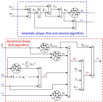
An overview of the first proposed distributed estimation algorithm is given in the scheme of Fig. 2. Each rectangular box in the scheme corresponds to a computation performed locally by each agent i. Each circle, instead, corresponds to a consensus-like distributed algorithm that is used to compute the only five global quantities that we shall prove to be needed in the distributed estimation process. The number of these global quantities is independent from the number of agents, and they can be estimated using standard distributed algorithms. Therefore, the overall distributiveness of the ap-proach is ensured. The convergence of the adopted distributed algorithms requires only that the overall communication graph is connected (no all-to-all communication is required). The same applies for our distributed estimation algorithm.
To better understand the overall functioning of the algo-rithm, it is convenient to logically decompose its structure in a purely kinematic phase, followed by a dynamical one. In the former, only the rigid body kinematics constraints and the velocity measurements are used. After this phase, each agent i is able to estimate the time-varying quantities zi(t)and !(t).
In the latter, the applied wrench and the rigid body dynamics are also used. After this phase, each agent is able to estimate the remaining quantities, i.e., J, zC(t), vC(t), and m. The
two phases are described in Sections IV and V, respectively. All the estimation blocks are cascaded, hence conver-gence/inconsistency issues of feedback estimation structures do not affect our scheme. A clarification about the convergence of our strategy is in order. Some steps of the estimation pro-cedure are achieved through averaging consensus algorithms, which are known to converge asymptotically. Although this aspect theoretically yields infinite convergence times, an ✏-approximate global consensus [18], up to an arbitrary accu-racy, can be achieved after a convenient finite time interval.
The first estimation algorithm assumes constant J and m and represents the best choice, in terms of noise filtering, in that case. The estimation of J requires a special wrench
fi= kzz?i zi 7 8 kz n X i=1 kzik2 J fi fmean ⌘1 zC 9 10 ! vCi vC fmean m 12 13 14 zi ! 11 ⌘2 ⌧i vCi vCj ˙zij ~yij dij zij 1 2 3 4 5 6 zi !
kinematic phase (first and second algorithm)
dynamical phase (first algorithm)
Fig. 2: Overview of the first proposed distributed estimation algo-rithm.Top (dashed blue box): purely kinematic phase, where only the velocity measurements and the rigid body kinematics are used. After this phase, the estimates of the time-varying quantities zi(t)and !(t)(in blue) become available to each agent i.Bottom (dashed red box): dynamical phase, where also the knowledge of the wrenches and the rigid body dynamics are used. After this phase, the quantities J, zC(t), vC(t), and m (in red) become available to each agent i.
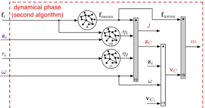
input, which prevents the use of another control algorithm in that phase. To overcome such possible drawbacks, a second estimation algorithm is also proposed. The second algorithm is designed as a variant of the first one, and described in Sec. VI, see Fig. 3. It can deal with changing J and m and does not require any particular wrench in any of its phases.
IV. KINEMATICPHASE
The objective of this phase is to distributively compute an estimate of the time-varying quantities zi(t) and !(t), based
only on the locally measured velocities and the rigid body kinematic constraints. The basic idea of this phase is to split the estimations of zi(t) and !(t) in two parts. The former
is common to both estimations and essentially consists of the estimation of zij(t) = pi(t) pj(t). This part is described
in Sec. IV-A. The latter comprises two separate estimators of zi(t)and !(t) and is described in Sec. IV-B
The reason for passing through the estimation of the quan-tities zij is briefly explained in the following. In [19], a
dis-tributed algorithm is proposed that allows the estimation of the centroid of the positions of a network of agents by only mea-suring the relative positions between pairs of communicating agents. This algorithm can be used to distributively estimate zi(t) if each pair of neighbors know the relative position of
the contact points Ci and Cj, i.e., zij(t). Nevertheless, here
each agent only measures the velocity of its contact point and not its position. Our first contribution is to show that, thanks to the rigid body constraint, it is possible to estimate zij(t)
to enhance readability, we shall drop the time dependence of variables where such a dependence is clear from the context. A. Estimation of zij(t)
The time-varying vector zij(t)that we want to estimate has
to obey to the nonlinear rigid body constraint
z>ijzij = const. (4)
This implies that, even though the direction of zij(t)may vary
in time, its norm kzijk is constant. Taking the time derivative
of both sides of (4) yields ˙z>
ijzij = 0, which implies that
the directions of zij and ˙z?ij = Q ˙zij coincide. We can then
explicitly decompose zij in two factors
zij = dij~yij, (5)
where ~yij = ˙z?ij k˙z?ijk 2 S1 is the unit vector denoting the
time-varying oriented line (axis) along which zij lies, and
dij 2 R is the coordinate of zij on ~yij.
Let each agent i send to all j 2 Nithe (measured) velocity
of its contact point vCi using the one-hop communication
links. Then, each agent i can compute the velocity difference ˙zij= vCi vCj, (6)
and the corresponding orthogonal vector ˙z?
ij, for each j 2 Ni.
As a consequence, ~yij is locally available to each agent i,
8j 2 Ni. This is the first milestone of our algorithm, which
is formally stated in the following result.
Result 1. The axis ~yij along which zij lies is directly
com-puted from local measurements and one-hop communication as ~yij = ˙z?ij/k˙z?ijk = (vCi vCj)?/kvCi vCjk, as long as
k˙zijk = kvCi vCjk 6= 0.
To obtain the sought zij, only the estimation of dij is left.
Due to the rigid body constraint (4), |dij| = kzijk = const
holds, i.e., dij is either equal to kzijk or to kzijk, depending
on the fact that ~yij and zij have the same or the opposite
direction. However, since in (5) both zij(t) and ~yij(t) are
continuous functions of time (for ~yij this holds in any open
interval in which k˙zijk 6= 0), we have that sign(dij) =
const 8t 2 T , as long as k˙zijk 6= 0, 8t 2 T . Thus, in any
time interval T in which k˙zijk 6= 0 and under the reasonable
assumption that the input wrenches are continuous in t over T, we can differentiate both sides of (5), thus obtaining
˙zij = dij˙~yij, (7)
which forms a linear estimation problem that agent i can locally solve to estimate the sought dij. In fact, among the
quantities that appear in (7), agent i knows the quantity ˙zijand
the time integral of d
dt~yij, i.e., ~yij. Therefore, the estimate of
dij can be carried out using a standard online linear estimation
technique described, e.g., in [20], and summarized in the Appendix of [21]. This technique has also the property of averaging out the possible measurement noise. To this aim, the time interval T can be tuned on the basis of the noise level that has to be averaged out in the velocity measurements.
Note that after the first estimation of dij there is no need to
further estimate |dij|, since this is a constant quantity. Thus,
the only signal to keep track of is sign(dij). This can be
in-stantaneously achieved by implementing two linear observers of the dynamic system (7): one that assumes sign(dij) = 1
and the other assuming sign(dij) = 1. Then, it is sufficient
to select, at each time-step, the observer that provides the best estimate in terms of, e.g., measurement residual.
To conclude the description of the algorithm, every time it happens to be k˙zijk = 0, the last estimate of zij is kept
frozen. In a real implementation the introduction of a suitable threshold to cope with the possible noise is recommended.
We summarize the results of this section in the following. Result 2. The vector zij is estimated locally by agent i and
j by the separate computation of two quantities
• ~yij(time-varying axis), computed directly from vCi vCj
(see Result 1)
• dij(norm-constant coordinate along ~yij), computed from
vCi vCj by solving (7) via filtering and applying online
Linear Least Squares (LLS).
This part of the algorithm is referred with blocks 1, 2, 3, and 4 in the diagram of Fig. 2.
B. Estimation of zi(t)and !(t)
The estimated quantities zij(t) provide a straightforward
way to estimate zi. This estimation phase corresponds to block
5 in the diagram of Fig. 2.
Result 3. Once the estimate of zij(t) is available to each
agent i, 8j 2 Ni, each agent i estimates zi by using the
centroid estimation algorithm described in [19].
In order to estimate the angular rate !, we use the following relation from rigid body kinematics
!zij= ˙z?ij, (8)
where ˙z?
ij is locally computed from (6), and zij is locally
estimated, as shown in Sec. IV-A. Multiplying both sides of (8) by z>
ij, we obtain that, for each pair of communicating agents
iand j, an estimate of ! is directly given by ! = z>ij˙z?ij z>ijzij
1
. (9)
Result 4. ! is locally computed using (9), where ˙zij comes
from direct measurement and one-hop communication and zij
from Result 2.
This part of the algorithm corresponds to block 6 in the diagram of Fig. 2. The use of (9) provides agent i with as many estimates of ! as the number of its one-hop neighbors |Ni|. In the ideal case of noiseless velocity measurements,
all those estimates are identical. In the case of noisy velocity measurements, this redundancy can be exploited to average out the noise either at the local level (e.g., by averaging the different estimates corresponding to each neighbor) or at the global level (by, e.g., using some dynamic consensus strategy among all agents [22]). Clearly, the order of the dynamic consensus algorithm used is strictly related to the time variations of ! and, therefore, to the time variations of its estimates [22]. Moreover, such consensus will theoretically
converge asymptotically. However, dynamic consensus algo-rithms, able to track the average of their dynamic inputs up to a given bound, can be used [23].
Clearly, a measurement of the angular rate ! can also be obtained equipping each agent with a gyroscope placed at the contact point. Nevertheless, one of the goals, and contributions, of our work is to show that this additional sensor is not strictly needed to accomplish the estimation task. Remark IV.1. This estimation approach relies on the agree-ment on a common reference frame. In fact, the measured velocities vCi used to estimate zi, are referred to the same
ref-erence frame. Two possible approaches can be put forward in real-world applications: i) agents should communicate to agree on a common reference frame, or ii) agents use additional sensors (i.e., vision, compass, or infrared array) to perform conversions between quantities related to different frames.
V. DYNAMICALPHASE
The objective of this phase (corresponding to the dashed red box in Fig. 2) is to estimate the remaining quantities, i.e., the (constant) rotational inertia J, the (time-varying) position zC(t) of the CoM of B relative to the geometric center G
of the contact points, the (time-varying) velocity of the CoM vC(t), and the (constant) mass m. The order in which they are
estimated follows a dependency hierarchy, since some phase needs information about the outcome of previous ones. Thus, the order of estimation cannot be altered without preventing the correct execution of the proposed strategy. This phase makes use of the velocity measurements vCi, the applied
wrench ui, as well as the rigid body kinematics and dynamics.
The basic operations executed in this phase are summarized in the following:
1) (estimation of J) we exploit the knowledge of zito apply
a particular input wrench that cancels the effect of zC
in (3), thus, obtaining a reduced dynamics in which J is the only unknown; then, we estimate J using LLS; 2) (estimation of zC(t)) we use all the previously estimated
quantities, the rotational dynamics in (3), and the rigid body constraint to recast the estimation of zC to a
nonlinear observation problem that can be locally solved by each agent with an observer designed by us;
3) (estimation of vC(t)) we use rigid body kinematics to
compute vC(t)from all the quantities estimated so far;
4) (estimation of m) we use a distributed estimation of the total force produced by the agents and vC(t) to finally
estimate the constant m using LLS. A. Estimation of J
Assuming J as a constant quantity, our strategy is to impose a specific wrench for a short time interval in order to let its estimate converge close enough to the real value. After this finite time interval, any wrench can be applied again. This feature enables the concurrent execution of estimation and ordinary manipulation tasks.
Let us isolate the rotational dynamics from (3) ˙! = 1 J n X i=1 z?i >fi+ 1 Jz ? C >Xn i=1 fi+ 1 J n X i=1 ⌧i, (10)
where: (i) J is the constant to be estimated; (ii) !(t) is locally known by each agent thanks to Result 4; (iii) zi(t)
is locally known by each agent thanks to Result 3; (iv) fi and
⌧i are locally known by each agent, since they are applied
by the agent itself; (v) zC is still unknown. If we were able
to eliminate zC from (10), then J would become the only
unknown in (10). It is easy to verify that the influence of zC
in (10) is eliminated if each agent i applies a force fi such
that Pn
i=1fi = 0. A possible choice is to set fi = kzz?i ,
where kz 6= 0 is an arbitrary constant. In fact, this choice
implies Pn
i=1fi = kz
Pn
i=1z?i = kzPi=1n (pCi pG)? =
kzQPni=1(pCi pG) = 0. Note that this force can be
computed by each agent in a distributed way, since ziis locally
known thanks to Result 3.
By applying fi = kzz?i , the rotational dynamics (10)
becomes ˙! = kzJ 1Pni=1kzik2+ J1Pni=1⌧i. In order to
further simplify the distributed computation, let us also impose ⌧i = 0, 8i = 1 . . . n, limited to the time interval in which J
is estimated. Hence, (10) is further simplified in ˙! = J 1kz
n
X
i=1
kzik2. (11)
Equation (11) expresses a linear relation where the only unknown is the proportionality factor J 1. In fact, ! and
kzkzik2 are locally known to each agent i, which implies
that the constant quantity kzPni=1kzik2 can be computed
distributively through an average consensus [24] right after the moment in which each agent is able to estimate zi (block
7 in the diagram of Fig. 2). Therefore, the estimation of J is recast in (11) as a LLS estimation problem that can be solved resorting to the same strategy used to estimate dijin (7) (block
8 in the diagram of Fig. 2). A summary follows.
Result 5. Each agent distributively computes the constant sum kzPni=1kzik2 using zi from Result 3 followed by average
consensus. Then, each agent i applies a force fi = kzz?i for
a given time interval, the moment of inertia J is distributively computed by solving the LLS problem (11).
Ideally, in a noise-free setting, every agent concludes this phase with the same estimate of J. In realistic settings, where noise is present, each agent may have a slightly different estimate of J. Hence, a standard average consensus algorithm can be executed to average out the noise and improve the esti-mate of J. Also, in this case such consensus will theoretically converge asymptotically, but the convergence to a bounded ball centered in the average can be achieved in finite time and detected by means of suitable distributed strategies [25]. B. Estimation of zC
The main idea behind the estimation of the time-varying quantity zC(t) is to rewrite (10) in order to let only the
following kinds of quantities appear (in addition to zC(t)): • global quantities that can be distributively estimated; • local quantities available from the problem setting
(mea-surements or inputs) or from the previous results. Next, we demonstrate that such a rewriting is possible and also that the estimation of zC(t)boils down to a solvable nonlinear
observation problem. Let us first decompose the local force fi(t)in two parts and recall two important identities
fi(t) = 1 n n X i=1 fi(t) + fi(t) = fmean(t) + fi(t), (12) n X i=1 z?i > = 0 and n X i=1 fi= 0. (13)
We can then rewrite (10), using (12) and (13), as ˙! = J 1⇣Pn i=1z?i >⌘ fmean + nJ 1z?C > fmean(t) + J 1Pn i=1z?i > fi+ + J 1z?C >Pn i=1 fi+ J 1Pni=1⌧i= nJ 1z?C > fmean | {z } z? C>¯f + J 1 n X i=1 z?i > fi | {z } ⌘1 + J 1 n X i=1 ⌧i | {z } ⌘2 , i.e., ˙! = z?C >¯f + ⌘ 1+ ⌘2. (14)
The global quantities1
• ¯f = n Jfmean, • ⌘1= J 1Pni=1z?i > fi= J 1Pni=1z?i > fi, and • ⌘2= J 1Pni=1⌧i
can be all distributively estimated in parallel using three instances of the dynamic consensus algorithm [22] (blocks 9, 10, and 11 in the diagram of Fig. 2). The choice of the specific dynamic consensus algorithm strongly depends on the nature of the tracked signals. A dynamic consensus algorithm like the one presented in [23] enables the estimate of its convergence time given the rate of convergence. The only mild assumption made is that the input signals are continuous and bounded (in [23], Theorem 5.1). The global quantity !(t) is known thanks to Result 4. The only unknown in (14) is zC(t).
Define ⌘ = ⌘1+ ⌘2. The following result holds:
Result 6. The rotational dynamics is given by ˙! = z?C
>¯f + ⌘,
(15) where !(t) is known thanks to Result 4 and ¯f(t) and ⌘(t) are locally known to each agent through distributed computation. We use Eq. (15) to form a dynamical system where ! and zC(t) are the state variables and ¯f and ⌘ are the inputs.
Recalling that zC is a constant-norm vector, rigidly attached
to the object, the following holds:
˙zC = ! z?C. (16)
Combining (15) and (16), we obtain the nonlinear system 8 > < > : ˙x1= x2x3 ˙x2= x1x3 ˙x3= x1u2 x2u1+ u3 , y = x3, (17) where zC= (zCx z y
C)> = (x1x2)>is the unknown part of the
state vector, ! = x3 is the measured part of the state vector
and, consequently, can be considered as the system output, and ¯f = ( ¯fxf¯y)> = (u1u2)>, ⌘ = u3 are known inputs.
1The same considerations made in Remark IV.1 are in order.
Result 7. Estimating zC(t)is equivalent to observe the state
(x1x2)> of the nonlinear system (17) with known output y =
x3= ! and known inputs u1= ¯fx, u2= ¯fy, and u3= ⌘.
In [26], we studied the observability of (17):
Proposition 1. If x36⌘ 0 and (u1u2)> 6⌘ 0, then system (17)
is locally observable in the sense of [27]. Proof. Given in [26].
Note that the applied torques ⌧i, for i = 1 . . . n (which
are included in u3) have no influence on the observability
of zC(t). In [28], an observability condition that involves
the angular velocity is also given. However, the condition expressed in [28] pertains the estimation of the kinematic parameters and requires that the direction of the angular velocity does not remain constant over the time, while in our setting the direction is constant and we only require that the norm is not constantly zero. In [26], we also proposed a nonlinear observer for system (17), which is summarized in the following result.
Proposition 2. Consider the following dynamical system 8 > < > : ˙ˆx1= xˆ2x3+ u2(y xˆ3) ˙ˆx2= ˆx1x3 u1(y xˆ3) ˙ˆx3= ˆx1u2 xˆ2u1+ ke(y xˆ3) + u3 , (18)
where ke > 0. If y(t) 6⌘ 0 and (u1(t) u2( t))> 6⌘ 0,
then (18) is an asymptotic observer for (17). Hence, defining ˆ
x = (ˆx1 xˆ2 xˆ3)> and x = (x1 x2 x3)>, one has that
ˆ
x(t)! x(t) asymptotically. Proof. Given in [26].
Thanks to Proposition 2 we can state the following result: Result 8. The relative position of the CoM w.r.t. the center of the contact points, i.e., zC(t), is distributively computed by
using the observer (18) and thanks to the local knowledge of n, J, !, fmean, and Pni=1z?i
>
fi from the previous results.
The estimation of zC(t) described beforehand is
schema-tized in blocks 9, 10, 11 (dynamic consensus algorithms) and 12(observer introduced in (18)) in the diagram of Fig. 2.
The inputs u1,2,3 of the observer arise from a dynamic
consensus phase. As already stated, dynamic consensus al-gorithms converge asymptotically, thus, only the convergence to a ball centered in the average of the values of nodes can be guaranteed in finite time, in dependence of the convergence rate [23]. For this reason, it is important to analyze what hap-pens to the observer’s state when an additive input disturbance is present. To this aim, we define eui= ui+"i, with i = 1, 2, 3
and analyze the dynamics of e = x xˆ 8 > < > : ˙e1= e2x3+eu2e3 ˙e2= e1x3 ue1e3 ˙e3= e1eu2 e2eu1 kee3 "3 . (19)
Defining the class K function2 (r) = r
ke(✓ 1), where 0 <
✓ < 1 and ke> 0, the following result holds.
Proposition 3. The error system of (18), i.e., (19), is Input-to-State Stable (ISS) with (r) = r
ke(✓ 1), where 0 < ✓ < 1
and ke> 0, according to Definition 4.7, [29].
Proof. Provided in the technical report associated with this paper, which can be downloaded at: https://arxiv.org/abs/1602. 01891
C. Estimation of vC
The velocity of the center of mass vC(t)is estimated locally
by each agent i using the rigid body constraint d
dt(pC pCi) =
!(pC pCi)?, which can be rewritten as
vC(t) = vCi(t) !(t)(zC(t) + zi(t))
?, (20)
whose right-hand-side elements are all known since:
• vCi(t) is locally measured by agent i
• !(t), zC(t), and zi(t)are known by each agent i thanks
to Results 4, 8, and 3, respectively.
Result 9. The CoM velocity vC(t)is distributively computed
using (20) and the knowledge of vCi(t), !(t), zC(t), zi(t).
Block 13 in the diagram of Fig. 2 represents this part. D. Estimation of the mass m
The estimation of the mass m is a straightforward conse-quence of the estimation of the vCi(t) and average force. In
fact, rewriting (2) as ˙vC=m1 Pni=1fi= mnfmean, we obtain
˙vC= m 1n fmean, (21)
where i) n is known, ii) fmeanis distributively estimated from
fi using dynamic consensus (as in Result 6), and iii) vC
is known locally by each agent i thanks to Result 9. Thus, the problem is recast as the linear least square estimation problem (21) that can be solved resorting to the same strategy used to estimate dij in (7) and J in (11).
Result 10. The mass m is distributively computed from the knowledge of v and n, and fmean by solving an online linear
least square problem via filtering (21).
Block 14 in the diagram of Fig. 2 represents this part. VI. INERTIA ANDMASSCHANGING DURING THETASK
In some particular cases, it might happen that the values of J and m change during the manipulation because, e.g., an object which was part of the load is dropped or, viceversa, a new object is added to the load. Such changes cause discrete jumps at certain instants in the values of J and m, which could be estimated again using the methods proposed in Sections V-A and V-D. However, in order to do so the robots would need to detect that J and m have changed and to trigger again the estimation algorithms. Furthermore, the estimation of J proposed in V-A requires that each agent applies a
2According to Definition 4.2, [29], a continuous function ↵ : [0, a) !
[0,1) is said to belong to class K if it is strictly increasing and ↵(0) = 0.
zi J fi fmean ⌘1 zC 9 10 ! vCi vC fmean m 15 13 16 zi ! 11 ⌘2 ⌧i dynamical phase (second algorithm)
Fig. 3: Overview of the dynamical phase for the second algorithm. Compared to the dynamical part of the first algorithm (Fig. 2) the consensus 7 and the step estimator 8 blocks are removed; while block 12is replaced by the new estimator (24) (new gray block 15); and block 14 is replaced by the new estimator (26) (new gray block 16).
specific force fi= kzz?i . However, in some cases it might be
inconvenient to temporarily pause the manipulation and apply such forces for estimating again J.
In order to deal with such possibilities we propose here a variant of the first estimation algorithm which is based on two new estimators, see Fig. 3. The first is an alternative observer that extends (18) including J in the state vector. Such estimation method can run in the background during the manipulation, thus overcoming all the aforementioned possible pitfalls. The second is a new observer for m that can also run in the background and does not need any trigger or special coordination among agents. Both observers are derived next.
Assuming that J is not known, Result 6 can be recast as: Result 11. The rotational dynamics is given by
˙! = J 1z?C
>˜f + J 1⌘,˜ (22)
where !(t) is known thanks to Result 4, and ˜f = nfmeanand
˜
⌘ = J⌘1+ J⌘2 =Pni=1z?i >
fi+Pni=1⌧i are locally known
to each agent through distributed computation.
Combining (22) and (16), and knowing the fact that ˙J = 0 at any time except in the few isolated instants in which the unknown load inertia undergoes discrete, step-like changes, we obtain an extended version of (17)
8 > > > < > > > : ˙x1= x2x3 ˙x2= x1x3 ˙x3= x4x1u2 x4x2u1+ x4u3 ˙x4= 0 , y = x3, (23) where (x1 x2)> = zC = (zCx z y
C)> and x4 = J 1 are the
unknown parts of the state vector, x3= !is its measured part
and, consequently, can be considered as the system output, and (u1u2)>= ˜f, u3= ˜⌘ are known inputs.
Proposition 4. Consider the following dynamical system ˙ˆx1= xˆ2x3+ u2(y xˆ3)
˙ˆx2= ˆx1x3 u1(y xˆ3)
˙ˆx3= ˆx1u2 xˆ2u1+ ˆx4u3+ ke(y xˆ3)
˙ˆx4= u3(y xˆ3),
where ke > 0. If y(t) 6⌘ 0, u3(t) 6⌘ 0 and (u1(t) u2(t))> 6⌘
0, then (24) is an asymptotic observer of a modified version of (23), in which the following change of variable is performed x1! x1x4, x2! x2x4. Thus, defining ˆx = (ˆx1 xˆ2 xˆ3 xˆ4)>
and x = (x1x4 x2x4 x3 x4)>, one has that ˆx(t) ! x(t)
asymptotically, which in turn implies that (ˆx1/ˆx4 xˆ2/ˆx4)!
(x1 x2)asymptotically.
Proof. Provided in the technical report associated with this paper, which can be downloaded at: https://arxiv.org/abs/1602. 01891
In the ideal case, the estimates carried out by all the robots are identical. In the case of noisy measurements, the noise can be averaged out by means of a dynamic consensus algorithm [23], as done for the estimation of !.
In order to observe m, we design an observer for the following nonlinear dynamical system
(
˙z1= z2u
˙z2= 0
, y = z1, (25)
which is easily derived from (21) by defining z1= vC,x+vC,y,
z2= m 1, u = fmean,x+fmean,y, and by imposing ˙m = 0 for
the same reasons for which it was previously assumed ˙J = 0. Proposition 5. Consider the following dynamical system
˙ˆz1= ˆz2u + k1(y zˆ1)
˙ˆz2= k2(y zˆ1),
(26) where k1, k2 2 R. If k1 > 0, k2u > 0, and k12> 4k2uhold,
then (26) is an asymptotic observer of (25).
Proof. Provided in the technical report associated with this paper, which can be downloaded at: https://arxiv.org/abs/1602. 01891
The same observation made for the estimation of a time-varying J is valid in this case: in the ideal case of noiseless measurements, the estimates carried out by all the robots are identical. In the case of noisy measurements, the noise can be averaged out by means of a dynamic consensus algorithm [23]. VII. DECENTRALIZEDOBSERVABILITY-BASEDCONTROL
In the previous sections, we have shown how to solve the Problem in Sec. II. Apart from the phase of the first-algorithm in which J is estimated (Sec. V-A), in all the other phases we did not suggest any control input to move the load and perform the estimation. The user of the algorithm is free to use any control input, as long as it ensures the observability conditions, i.e., non-zero angular rate ! and non-zero average force fmean.
In each phase, either one or both of the two conditions are needed to ensure a convergent estimation.
In the following, we prove that an extremely basic control strategy satisfies, under very mild conditions, the aforemen-tioned observability requirements. Furthermore, this control strategy: (i) can be implemented relying only on local perception and communication (it is, therefore, distributed); and (ii) does not require the knowledge of parameters and quantities that are the objectives of the distributed estimation
(it is estimation-‘agnostic’). Hence, it can be applied during the estimation process and independently from it.
Proposition 6. Assume that the following local control rule is used: fi = f⇤= const, ⌧i = 0, 8i = 1 . . . n, and denote with
!0 the rotational rate at t = 0, then
1) !(t) remains bounded, in particular: |!(t)| q!2
0+ 4nJ 1kf⇤kkzCk 8t 0 (27)
2) 9¯t 0 such that ! becomes ! ⌘ 0 8t ¯t, if and only if the following condition hold
2nzC(0)>f⇤ J!2(0) = 2nkzCkkf⇤k. (28)
Thus, the proposed control law is suitable for the estimation process apart from a zero-measure case implied by (28). Proof. Provided in the technical report associated with this paper, which can be downloaded at: https://arxiv.org/abs/1602. 01891
The use of the local control action in Proposition 6 ensures the sought observability conditions under the very mild con-ditions specified in (28). However, it causes the load CoM velocity to grow linearly over time (see, e.g., (21)). Therefore, it is wise to modify the proposed control action by periodically changing the direction of the common force (i.e., switching between f⇤ and f⇤ on a periodical basis). In this way, the
CoM velocity will boundedly oscillate around zero.
It is also important to define a control strategy that is able to stop the load motion if needed (like, e.g., at the end of all the estimation phases). This is provided in the following. Proposition 7. Assume that the following local control rule is used: fi = bvCi, ⌧i= 0, 8i = 1 . . . n, with b > 0. Then, both
!and vC converge asymptotically to zero with a convergence
rate that is proportional to b.
Proof. Provided in the technical report associated with this paper, which can be downloaded at: https://arxiv.org/abs/1602. 01891
VIII. NUMERICALRESULTS
This section and the Appendix show numerical results that validate our approach. First, we demonstrate the working prin-ciples of the first algorithm simulating a network of n = 10 agents manipulating an unknown load on a plane. Then, the validity of the first algorithm is extensively assessed through a detailed simulation campaign in a wide range of operational conditions. Finally we show some simulations for the second algorithm using time-varying mass and inertia observers. A. Manipulation of an unknown load by a team of 10 agents
We consider a planar load with m = 50 kg and J = 86.89kg m2, manipulated by a team of n = 10 agents
communicating over a line-topology network. Such a topology is the worst case for the algorithm convergence rate, which is an increasing function of the network diameter [30]. The velocity measurements are affected by an additive zero-mean Gaussian noise with covariance matrix ⌃i = 2I2⇥2, and
t6= 180 t5= 135 t4= 80 t3= 40 t2= 30 t1= 10
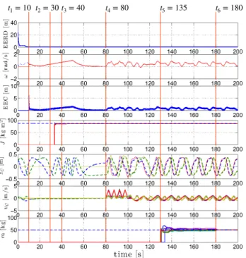
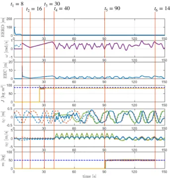
Fig. 4: An illustrative simulation of the whole estimation algorithm described in Secs. IV and V. From top to bottom, respectively: the trend of the EERD index, the estimates of !, the trend of the EEC index, the estimates of J, the observations of zC, the estimates of vC, and the estimates of m. Dashed lines indicate true values, while solid lines indicate estimates.
= 0.3 m/s. The quantities involved in the execution and assessment of the first algorithm are illustrated in Fig. 4.
As a first step, starting from t0 = 0, each agent applies
an arbitrary force and executes the procedure described in Sec. IV-A to estimate the relative distances between contact points. We observe that the presence of noise in the velocity measurements can make the signal-to-noise ratio too small to make an effective use of acquired measurement. In this case, we opt for keeping the last valid measurement as constant, and not to update the measurement with quantities that are too noisy to be useful. The signal-to-noise ratio threshold in order to consider the measured velocity is set to k˙zijk 0.5
m/s. The first plot of Fig. 4 reports the convergence to zero of the Estimation Error Relative Distance (EERD) index, defined as EERD(t) =Pn 1
i=1
Pn
j=iA(i, j)k(zij(t) ˆzij(t))k2, where
variable ˆzij indicates the estimate of zij. Consistently, here
and henceforth, the estimate of a quantity ? is indicated with a superimposed hat, i.e., ˆ?. Dynamic consensus blocks have been implemented by means of the Fist Order Input Dynamic Consensus Filter [23] with parameter values set as ✏ = 0.01 and = 10. Static average consensus detection is detected by means of the method presented in [25]. Starting from t1 = 10s, each agent applies the control rules given in
Propositions 6 and 7, which guarantee both the observability and boundedness of ⇥v>
C !
⇤>. At t
1= 10s, ! and zi start to
be estimated, as described in Sec. IV-B. The second and third plots of Fig. 4 illustrate, respectively, the trend of the angular velocity ! and its estimate ˆ!, and the quadratic performance index on the estimation of the relative distance to the center of mass, i.e., EEC(t) =Pn
i=1k(zi(t) ˆzi(t))k2. At t = 20 s,
the first step of the dynamical phase is executed, as described in Sec. V-A. First, each agent runs an average consensus in order to locally estimate the constant value kzPni=1kzik2.
Such consensus will theoretically converge asymptotically. However, we use the technique presented in [25] to assess a suitable stopping condition. Specifically, we distributively determine when the consensus has been reached within a given error bound, which in our experiment is set to 0.001 m. At t3 = 30s each agent i runs a least square estimation of
J using also the knowledge of ˆ!. Each agent checks the convergence of the least squares estimation evaluating the variance of the estimator [31]. From t3 = 40s, the local
estimates are transmitted over the network and an average consensus is run to agree on a common estimate, which in our case is ˆJ = 85.67kg m2 (fourth plot in Fig. 4). Also in this case, we use the technique presented in [25] with error bound set to 0.01 kg m2. Then, the angular rate is brought to
zero (Proposition 7). Afterwards, at t4= 80s each agent starts
the nonlinear observation of zC described in Sec. V-B. The
observer errors reach zero at about t5 = 135s, as illustrated
in the fifth plot of Fig. 4. The estimate ˆvC is then computed
using (20) (sixth plot of Fig. 4), which in turn allows to compute ˆm, as explained in Sec. V-D, by a preliminary collections of samples and local least squares estimations. An average consensus phase, starting at t6 = 180s, leads to an
accurate estimate of m at tf = 200s (seventh and last plot of
Fig. 4). The same techniques previously described to detect consensus convergence [25] is applied here using a bound of 0.01kg. The duration of the entire algorithm is 200 s, of which a large portion is needed to collect samples to run the local least squares and the consensus algorithms for the constant parameters m, J and dij. The duration of these phases depends
on the noise level. Ideally, in the absence of noise, a single sample would be sufficient to perform the estimation, while in the real, noisy case, a trade-off between robustness [20] and duration of the estimation phase is necessary. Finally, also the convergence time of ˆzC can be shortened by acting on the
value of ke in (18), and the gains of the consensus algorithms
can be tuned in order to speed up the agreement [24]. Additional extensive results are given in the Appendix.
IX. CONCLUSIONS
In this paper, we propose two fully-distributed methods for the estimation of the parameters needed by a planar multi-agent system to collectively manipulate an unknown load, i.e., the kinematic and dynamic parameters, as well as the estimate of the kinematic state of the load, i.e., the velocity of the center of mass and its rotational rate. The approaches are totally distributed and rely on the geometry of the rigid body kinematics, on the rigid body dynamics, on nonlinear observation theory, and on consensus strategies. They are based on a sequence of steps that leads to states in which all agent agrees on the estimated parameters, during such steps any motion control law can be used (apart from a single step in the first algorithm). The only requirements are related to the communication network, which is only required to be connected, and to the capability of each agent to control
t1= 8 t 2= 16
t3= 30t
4= 40 t5= 90 t6= 140
Fig. 5: Simulation with the same setup as in Fig. 4, but with a fully connected topology and noise = 0.3m/s.
the local force applied to the load, while measuring the velocity of the contact point. Extensive numerical simulations confirm the effectiveness of our approach and its robustness to measurement noise and system size. Future works will deal with the manipulation of 3D objects in the aereal domain, extending the aerial manipulation methods in [32]–[34].
APPENDIX
A. Manipulation of an unknown load by a team of 10 agents Figures. 5 and 6 illustrate the same simulation setup of Sec. VIII-A in the case of a fully connected topology and two different levels of noise. Comparing the time sequence t1. . . t6, we observe that a more connected topology and a
lower noise level are factors that sensibly reduce the execution time of each
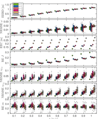
step.-B. Performance Assessment and Uncertainty Propagation We analyze the performance of the algorithm by running a Monte Carlo simulation campaign. Specifically, a wide range of operational conditions is considered, defined by the pair (n, ) where n indicates the number of agents in the network and the standard deviation defining the covariance of a zero-mean Gaussian noise, added to velocity measurements, as ⌃i= 2I2⇥2, for each agent i = 1, . . . , n.
The two parameters assume values over a 2D grid formed with the values n 2 {5, 8, 11, 14, 17, 20} and 2 {0.1, 0.2, 0.3, . . . , 1} m/s. Fifty independent simulations are run for each parameter pair. To ensure consistency of compar-ison in each simulation the mass is set as m = 5 n kg (and the inertia J is computed accordingly). The agents communicate over the worst-case line-topology.
Figure 7 illustrates the results, where each box-plot cor-responds to the 50 independent simulations executed for a
t1= 2 t2= 10t3= 14 t4= 30 t5= 63 t6= 95
Fig. 6: Simulation with the same setup as in Fig. 4, but with a fully connected topology and noise = 0.0001m/s.
given parameter pair. For consistency of comparison across the changing n, we use the Normalized Root Mean Square Error (NRMSE) and the Relative Error (RE), respectively for time-varying and constant parameters. The results show that the estimation accuracy decreases with an increasing noise level for the EERD, the EEC, the estimation of !, the estimation of vC, and the estimation of J. On the contrary, the
degradation in the estimation accuracy is of minor importance in the estimation of m. We observe that the error in the estimation of J is strongly dependent on n: fixing a value for , the estimation accuracy increases with an increase in the number of agents. This is related to the use of the consensus algorithm for averaging out the noise, as will be better shown later in this section. On the other hand, fixing the value for , the dispersion of the RE in the estimation of m increases with increasing n. This behavior is related to the greater number of noisy measurements used to estimate vC, used in turn to
estimate m. The degree of dispersion of the estimation of ! is clearly influenced by the noise level, the dispersion is close to zero for the EERD, EEC, and for the error in the estimation of J. Finally, fixing the number of agents n, the degree of the dispersion is constant with respect to the noise variation for the estimation error of vC and m, confirming that the estimation
of vC and m is strongly influenced by the level of noise.
As already mentioned in Sec. V-A, for the estimation of constant parameters, such as J and m, an average consensus algorithm is executed to average out the noise and improve the estimate. Figure 8 shows the box-plots of the RE of the estimation of J and m, before (on the left side) and after (on the right side) the average consensus run. We observe that the application of the average consensus algorithm decreases sig-nificantly the average estimation error and also the dispersion.
0.1 0.2 0.3 0.4 0.5 0.6 0.7 0.8 0.9 1 EERD [m] 0 0.5 1 1.5 n=5 n=8 n=11 n=14 n=17 n=20 0.1 0.2 0.3 0.4 0.5 0.6 0.7 0.8 0.9 1 NR M S E ω 0 0.01 0.02 0.03 0.1 0.2 0.3 0.4 0.5 0.6 0.7 0.8 0.9 1 EEC [m] 0.15 0.2 0.25 0.3 0.1 0.2 0.3 0.4 0.5 0.6 0.7 0.8 0.9 1 RE J 0.1 0.2 0.3 0.1 0.2 0.3 0.4 0.5 0.6 0.7 0.8 0.9 1 NR M S E vCx 0 0.05 0.1 0.1 0.2 0.3 0.4 0.5 0.6 0.7 0.8 0.9 1 NR M S E vCy 0 0.1 0.2 0.3 σ[m/s] 0.1 0.2 0.3 0.4 0.5 0.6 0.7 0.8 0.9 1 RE m 0 0.2 0.4 0.6
Fig. 7: Box-plots obtained by running the whole algorithm in different operational conditions, selected by setting the pair (n, ). The bottom of a box indicates the first quartile, while the top indicates the third quartile. The dot inside a box is the second quartile, i.e., the median. The whisker at the bottom/top of a box indicates the lowest/highest data within 1.5 of the Interquartile Range of the lower/upper quartile.
RE J 0.1 0.15 0.2 0.25 0.3 n=5n=8 n=11 n=14 n=17 n=20 0.1 0.15 0.2 0.25 0.3 σ[m/s] 0.1 0.2 0.3 0.4 0.5 0.6 0.7 0.8 0.9 1 RE m 0 0.5 1 1.5 σ[m/s] 0.1 0.2 0.3 0.4 0.5 0.6 0.7 0.8 0.9 1 0 0.5 1 1.5
Fig. 8: Box-plots of the Relative Error (RE) of the estimation of m and J obtained by running the whole algorithm in different conditions described by the pairs (n, ). The left and right column show the RE’s before and after running the average consensus, respectively.
C. Inertia Moment and Mass Changing along the Task To show the ability of the second algorithm to deal with changing m and J we simulate a planar load with m = 50 kg and J = 86.89 kg m2, manipulated by a team of n = 10 agents
communicating over a line-topology network and implement-ing the observers introduced in Sec. VI. A zero-mean Gaussian noise with covariance matrix ⌃i= 2I2⇥2and = 0.3 m/s is
added to the velocity measurements . After 100s, we simulate a step-like decrease of mass m and, consequently, a decrease of the moment of inertia J. Simulation results are illustrated in Fig. 9. As theoretically proven, both the observers converge
0 50 100 150 200 m − 1[kg − 1] 0 0.1 0.2 0.3 0 50 100 150 200 J − 1[kg − 1m − 2] 0 0.1 0.2 0.3
Fig. 9: Simulation of the performance of the observer for the time-varying inertial parameters described in Sec. VI. To: estimates of m 1. Bottom: the estimates of J 1. Dashed lines indicate true values, while solid lines indicate estimates.
to a bounded region around the new true values. REFERENCES
[1] K. I. Kim and Y. F. Zheng, “Two strategies of position and force control for two industrial robots handling a single object,” Robotics and Autonomous Systems, vol. 5, no. 4, pp. 395–403, 1989.
[2] S. A. Schneider and R. H. Cannon, “Object impedance control for cooperative manipulation: theory and experimental results,” IEEE Trans. on Robotics and Automation, vol. 8, no. 3, pp. 383–394, 1992. [3] I. D. Walker, R. A. Freeman, and S. I. Marcus, “Analysis of motion and
internal loading of objects grasped by multiple cooperating manipula-tors,” Robotics and Autonomous Systems, vol. 10, no. 4, pp. 396–409, 1991.
[4] J. Szewczyk, F. Plumet, and P. Bidaud, “Planning and controlling cooperating robots through distributed impedance,” Journal of Robotic Systems, vol. 19, no. 6, pp. 283–297, 2002.
[5] D. Sieber, F. Deroo, and S. Hirche, “Formation-based approach for multi-robot cooperative manipulation based on optimal control design,” in 2013 IEEE/RSJ Int. Conf. on Intelligent Robots and Systems, Tokyo, Japan, Nov. 2013, pp. 5227–5233.
[6] Y. Yong, T. Arima, and S. Tsujio, “Inertia parameter estimation of planar object in pushing operation,” in 2005 IEEE Int. Conf. on Information Acquisition, Hong Kong and Macau, China, June 2005, pp. 356–361. [7] D. Kubus, T. Kroger, and F. M. Wahl, “On-line estimation of inertial
parameters using a recursive total least-squares approach,” in 2008 IEEE/RSJ Int. Conf. on Intelligent Robots and Systems, Nice, France, Sep. 2008, pp. 3845–3852.
[8] S. Erhart and S. Hirche, “Adaptive force/velocity control for multi-robot cooperative manipulation under uncertain kinematic parameters,” in 2013 IEEE/RSJ Int. Conf. on Intelligent Robots and Systems, Tokyo, Japan, Nov. 2013, pp. 307–314.
[9] J. Markdahl, Y. Karayiannidis, X. Hu, and D. Kragic, “Distributed cooperative object attitude manipulation,” in 2012 IEEE Int. Conf. on Robotics and Automation, St. Paul, MN, May 2012, pp. 2960–2965. [10] Z. Wang and M. Schwager, “Multi-robot manipulation with no
com-munication using only local measurements,” in 54rd IEEE Conf. on Decision and Control, Osaka, Japan, Dec. 2015, pp. 380–385. [11] P. Culbertson and M. Schwager, “Decentralized adaptive control for
collaborative manipulation,” in 2018 IEEE Int. Conf. on Robotics and Automation, Brisbane, Australia, May 2018, pp. 278–285.
[12] A. Marino and F. Pierri, “A two stage approach for distributed coopera-tive manipulation of an unknown object without explicit communication and unknown number of robots,” Robotics and Autonomous Systems, vol. 103, pp. 122–133, 2018.
[13] G. Tel, Introduction to Distributed Algorithms. Cambridge University Press, 2000.
[14] B. Francis and M. Maggiore, “Models of mobile robots in the plane,” in Flocking and Rendezvous in Distributed Robotics, B. Francis and M. Maggiore, Eds. Springer, 2017, pp. 7–23.
[15] D. Prattichizzo and J. C. Trinkle, “Grasping,” in Springer Handbook of Robotics, B. Siciliano and O. Khatib, Eds. Springer, 2008, pp. 671–700. [16] A. Petitti, A. Franchi, D. Di Paola, and A. Rizzo, “Decentralized motion control for cooperative manipulation with a team of networked mobile manipulators,” in 2016 IEEE Int. Conf. on Robotics and Automation, Stockholm, Sweden, May 2016, pp. 441–446.
[17] P. Robuffo Giordano, A. Franchi, C. Secchi, and H. H. B¨ulthoff, “A passivity-based decentralized strategy for generalized connectivity maintenance,” The International Journal of Robotics Research, vol. 32, no. 3, pp. 299–323, 2013.
[18] N. E. Manitara and C. N. Hadjicostis, “Distributed stopping for average consensus in digraphs,” IEEE Trans. on Control of Network Systems, 2017.
[19] R. Aragues, L. Carlone, C. Sagues, and G. Calafiore, “Distributed cen-troid estimation from noisy relative measurements,” Systems & Control Letters, vol. 61, no. 7, pp. 773–779, 2012.
[20] J. J. E. Slotine and W. Li, Applied nonlinear control. Prentice Hall, 1991.
[21] A. Franchi, A. Petitti, and A. Rizzo, “Distributed estimation of the inertial parameters of an unknown load via multi-robot manipulation,” in 53rd IEEE Conf. on Decision and Control, Los Angeles, CA, Dec. 2014, pp. 6111–6116.
[22] M. Zhu and S. Martinez, “Discrete-time dynamic average consensus,” Automatica, vol. 46, no. 2, pp. 322–329, 2010.
[23] S. S. Kia, J. Cort´es, and S. Mart´ınez, “Singularly perturbed algorithms for dynamic average consensus,” in 2013 European Control Conference, Zurich, Switzerland, Dec. 2013, pp. 1758–1763.
[24] R. Olfati-Saber, J. A. Fax, and R. M. Murray, “Consensus and coop-eration in networked multi-agent systems,” Proceedings of the IEEE, vol. 95, no. 1, pp. 215–233, 2007.
[25] V. Yadav and M. Salapaka, “Distributed protocol for determining when averaging consensus is reached,” in 2007 45th Allerton Conf. on Commu-nications, Control and Computing, Monticello, IL, Sep. 2007, p. 715720. [26] A. Franchi, A. Petitti, and A. Rizzo, “Decentralized parameter estimation and observation for cooperative mobile manipulation of an unknown load using noisy measurements,” in 2015 IEEE Int. Conf. on Robotics and Automation, Seattle, WA, May 2015, pp. 5517–5522.
[27] R. Hermann and A. J. Krener, “Nonlinear controllability and observ-ability,” IEEE Trans. on Automatic Control, vol. 22, no. 5, pp. 728–740, 1977.
[28] F. Aghili, “Adaptive control of manipulators forming closed kinematic chain with inaccurate kinematic model,” IEEE/ASME Trans. on Mecha-tronics, vol. 18, no. 5, pp. 1544–1554, 2013.
[29] H. K. Khalil, Nonlinear Systems, 3rd ed. Prentice Hall, 2001. [30] A. Olshevsky and J. N. Tsitsiklis, “Convergence speed in distributed
consensus and averaging,” SIAM Review, vol. 53, no. 4, pp. 747–772, 2011.
[31] S. Van de Geer, “Least squares estimators,” ser. Encyclopedia Statistics in The Behavioral Sciences, B. Everitt and D. Howell, Eds. John Wiley, 2005.
[32] G. Gioioso, A. Franchi, G. Salvietti, S. Scheggi, and D. Prattichizzo, “The Flying Hand: a formation of UAVs for cooperative aerial tele-manipulation,” in 2014 IEEE Int. Conf. on Robotics and Automation, Hong Kong, China, May. 2014, pp. 4335–4341.
[33] G. Gioioso, M. Ryll, D. Prattichizzo, H. H. B¨ulthoff, and A. Franchi, “Turning a near-hovering controlled quadrotor into a 3D force effector,” in 2014 IEEE Int. Conf. on Robotics and Automation, Hong Kong, China, May. 2014, pp. 6278–6284.
[34] B. Y¨uksel, C. Secchi, H. H. B¨ulthoff, and A. Franchi, “Reshaping the physical properties of a quadrotor through IDA-PBC and its application to aerial physical interaction,” in 2014 IEEE Int. Conf. on Robotics and Automation, Hong Kong, China, May. 2014, pp. 6258–6265.
Antonio Franchi (S’07-M’11-SM’16) received the Ph.D. degree in system engineering from Sapienza University of Rome, Rome, Italy, in 2010 and the Habilitation to Direct Research (HDR) in Sciences from National Polytechnic Institute of Toulouse, Toulouse, France, in 2016. In 2009, he was a Visiting Scholar with University of California at Santa Bar-bara, Santa BarBar-bara, CA, USA. From 2010 to 2014, he was Research Scientist, Senior Research Scientist, and the Project Leader of the Autonomous Robotics and Human Machine Systems Group, Max Planck Institute for Biological Cybernetics in T¨ubingen, Germany. Since 2014, he has been a Tenured CNRS Researcher with the RIS team, LAAS-CNRS, Toulouse, France. He published more than 120 papers in peer-reviewed international journals and conferences. His main research interests include robotic systems, with a special regard to control of for aerial robots and multiple-robot systems. Dr. Franchi received the IEEE RAS ICYA Best Paper Award in 2010. He is an Associate Editor for IEEE TRANSACTIONS ON ROBOTICS. He is the co-founder of the IEEE RAS Technical Committee on Multiple Robot Systems and of the International Symposium on Multi-Robot and Multi-Agent Systems.
Antonio Petitti received the B.S. and M.S. (Laurea Specialistica) degrees (summa cum laude) in Au-tomation Engineering from Politecnico di Bari, Italy, in 2008 and 2010, respectively. From June 2011 to May 2018, he was Research Assistant at the Insti-tute of Intelligent Systems for Automation (ISSIA) of the National Research Council (CNR), Italy. In 2015, he received the Ph.D. degree in Electrical and Information Engineering at Politecnico di Bari, Italy, and the joint Ph.D. degree of high qualification Scuola Interpolitecnica di Dottorato in Information and Communication Technologies. In 2013 and 2014 he was Visiting Research Fellow at ARHMS group, Max Planck Institute for Biological Cybernetics, T¨ubingen, Germany, and at RIS group LAAS-CNRS, Toulouse, France, respectively. Since June 2018, he has been Researcher at the Institute of Intelligent Industrial Technologies and Systems for Advanced Manufacturing (STIIMA) of the CNR, Bari, Italy. His scientific interests are focused on consensus theory and applications, distributed estimation, modeling and control of robotic networks.
Alessandro Rizzo received the Laurea degree (summa cum laude) in computer engineering and the Ph.D. degree in automation and electronics engineer-ing from the University of Catania, Italy, in 1996, and 2000, respectively. He is an Associate Professor at Politecnico di Torino, Italy, where he is engaged in conducting and supervising research on cooperative robotics, complex networks and systems, modeling and control of nonlinear systems. Since 2012, he has also been a Visiting Professor at the New York University Tandon School of Engineering, Brooklyn, NY, USA. He is the author of two books, two international patents, and more than 130 papers on international journals and conference proceedings. Prof. Rizzo has been the recipient of the award for the best application paper at the IFAC world triennial conference in 2002 and of the award for the most read papers in Mathematics and Computers in Simulation (Elsevier) in 2009. Prof. Rizzo is also a Distinguished Lecture of the IEEE Nuclear and Plasma Science Society. More details can be found at the website staff.polito.it/alessandro.rizzo.
Proofs of Propositions
Technical report associated with the paper:
“Distributed Estimation of State and Parameters in Multi-Agent Cooperative Load Manipulation”
IEEE Transactions on Control of Network Systems
Antonio Franchi, Antonio Petitti, Alessandro Rizzo
Abstract—This document is a technical attachment to [1]. Here, we present the proofs of the Propositions.
I. HOW TOCITE THISWORK
This technical report is accompanying the IEEE Transac-tions on Control of Network Systems paper [1]. If you wish to reference this work, please cite this paper as follows:
@ A r t i c l e { F r a n c h i 1 9 t c n s ,
a u t h o r = {A. F r a n c h i and A. P e t i t t i and A. Rizzo } ,
t i t l e = { D i s t r i b u t e d E s t i m a t i o n of S t a t e and P a r a m e t e r s i n Multi Agent C o o p e r a t i v e Load M a n i p u l a t i o n } , j o u r n a l = {{IEEE} T r a n s a c t i o n s on C o n t r o l o f Network Systems } , y e a r = {TBD} , d o i = {TBD} , }
Proof of Proposition 3 in [1]. In the ideal case withe1,2,3=
0, the origin of the system in (19) is asymptotically stable (Theorem V.1, [2]). Consider the following Lyapunov function V (e) =1 2e>e, then ˙V = e1e2x3+e1eu2e3+e2e1x3 e2ue1e3+ . . . e3e1ue2 e3e2eu1 kee23 e3e3 = kee23 e3e3 kee23+|e3||e3|. (TR.1) We observe that kee23+|e3||e3| = = kee23+|e3||e3| + kee21 kee21+kee22 kee22 = kekek2+|e3||e3| + kee21+kee22. (TR.2) Considering that kek |e3| and keeek |e3|, we have that
˙V kekek2+|e3||e3| + kee21+kee22
kekek2+kekkeeek + kee21+kee22.
(TR.3)
A. Franchi is with CNRS, LAAS, 7 avenue du colonel Roche, F-31400 Toulouse, France and Univ de Toulouse, LAAS, F-31400 Toulouse, France
A. Petitti is with the Institute of Intelligent Industrial Technologies and Systems for Advanced Manufacturing, National Research Council (STIIMA-CNR), 70126 Bari, Italy,[email protected]
A. Rizzo is with the Dipartimento di Elettronica e Telecomunicazioni, Politecnico di Torino, Corso Duca degli Abruzzi 24, 10129 Torino, Italy
This research was partially supported by the ANR, Project ANR-17-CE33-0007 MuRoPhen, by the Siebel Energy Institute, and by Compagnia di San Paolo.
Moreover, considering that kekek2 kee21+kee22, we can write
˙V kekek2+kekkeeek + kee21+kee22
kekek2+kekkeeek + kekek2. (TR.4)
Thus, we rewrite the foregoing inequality as
˙V ke(1 q)kek2 keqkek2+kekkeeek + kekek2, (TR.5)
where 0 < q < 1. The inequality keqkek2+kekkeeek +
kekek2 0 holds if kek ke(q 1)keeek . Thus,
˙V ke(1 q)kek2,8kek k keeek
e(q 1). (TR.6)
Hence, the system is ISS (Theorem 4.19, [3]).
Proof of Proposition 4 in [1]. Define the error vector as e = [e1e2e3e4]> =
[(x1x4 ˆx1) (x2x4 ˆx2) (x3 ˆx3) (x4 ˆx4)]>. After some
algebra, the error dynamics is given by ˙ e = 2 6 6 4 0 x3 u2 0 x3 0 u1 0 u2 u1 ke u3 0 0 u3 0 3 7 7 5e = [U + diag(0,0, ke,0)]e, (TR.7) where U is skew symmetric, i.e., U + U>=0. Define the
following candidate Lyapunov function: V (e) = 1
2e>e, whose
time derivative along the system trajectories is ˙V = e>e = e˙ >Ue kee2
3= kee23, (TR.8)
which is negative semidefinite. Now in order to study the invariant set that ensures that ˙V = 0 we impose that e3⌘ 0,
which implies, in particular, that e3=0, ˙e3=0, and ¨e3=0.
Considering, for simplicity, the case in which inputs are stepwise constant, the last three equations (24)–(TR.8) result in the following system of linear equations:
2 4 xu32u1 xu3u12 u03 x2 3u2 x23u1 0 3 5 2 4ee12 e4 3 5 = E 2 4ee12 e4 3 5 = 2 400 0 3 5. (TR.9) The determinant of E is u3x33(u21+u32). If the assumptions
of the theorem hold, then E is nonsingular and therefore the only trajectory of the system that ensures ˙V = 0 ise = 0. Proof of Proposition 5 in [1]. Define the error vector e = (e1 e2)>= (z1 ˆz1z2 ˆz2)>. The error dynamics is given by
˙
e = k1 u