HAL Id: insu-02403865
https://hal-insu.archives-ouvertes.fr/insu-02403865
Submitted on 11 Dec 2019
HAL is a multi-disciplinary open access archive for the deposit and dissemination of sci-entific research documents, whether they are pub-lished or not. The documents may come from teaching and research institutions in France or abroad, or from public or private research centers.
L’archive ouverte pluridisciplinaire HAL, est destinée au dépôt et à la diffusion de documents scientifiques de niveau recherche, publiés ou non, émanant des établissements d’enseignement et de recherche français ou étrangers, des laboratoires publics ou privés.
Mapping gas exchanges in headwater streams with
membrane inlet mass spectrometry
Camille Vautier, Ronan Abherve, Thierry Labasque, Anniet M. Laverman, Aurélie Guillou, Eliot Chatton, Patrick Dupont, Luc Aquilina, Jean-Raynald
de Dreuzy
To cite this version:
Camille Vautier, Ronan Abherve, Thierry Labasque, Anniet M. Laverman, Aurélie Guillou, et al.. Mapping gas exchanges in headwater streams with membrane inlet mass spectrometry. Journal of Hydrology, Elsevier, 2020, 581, pp.124398. �10.1016/j.jhydrol.2019.124398�. �insu-02403865�
Journal Pre-proofs
Research papers
Mapping gas exchanges in headwater streams with membrane inlet mass spec-trometry
Camille Vautier, Ronan Abhervé, Thierry Labasque, Anniet M. Laverman, Aurélie Guillou, Eliot Chatton, Pascal Dupont, Luc Aquilina, Jean-Raynald de Dreuzy
PII: S0022-1694(19)31133-3
DOI: https://doi.org/10.1016/j.jhydrol.2019.124398
Reference: HYDROL 124398 To appear in: Journal of Hydrology
Received Date: 26 July 2019 Revised Date: 20 November 2019 Accepted Date: 22 November 2019
Please cite this article as: Vautier, C., Abhervé, R., Labasque, T., Laverman, A.M., Guillou, A., Chatton, E., Dupont, P., Aquilina, L., de Dreuzy, J-R., Mapping gas exchanges in headwater streams with membrane inlet mass spectrometry, Journal of Hydrology (2019), doi: https://doi.org/10.1016/j.jhydrol.2019.124398
This is a PDF file of an article that has undergone enhancements after acceptance, such as the addition of a cover page and metadata, and formatting for readability, but it is not yet the definitive version of record. This version will undergo additional copyediting, typesetting and review before it is published in its final form, but we are providing this version to give early visibility of the article. Please note that, during the production process, errors may be discovered which could affect the content, and all legal disclaimers that apply to the journal pertain.
1 Mapping gas exchanges in headwater streams with membrane inlet mass
2 spectrometry
3 Camille Vautier a*, Ronan Abhervé a,b , Thierry Labasque a,c , Anniet M.
4 Laverman d , Aurélie Guillou c , Eliot Chatton a,1 , Pascal Dupont e , Luc Aquilina a ,
5 Jean-Raynald de Dreuzy a,c
6 a Univ Rennes, CNRS, Géosciences Rennes, UMR 6118, 35000 Rennes, France
7 b Centre Eau Terre Environnement, INRS, Quebec City, Canada
8 c Univ Rennes, CNRS, OSUR (Observatoire des sciences de l’univers de Rennes),
9 UMS 3343, 35000 Rennes, France
10 d Univ Rennes, CNRS, Ecobio, UMR 6553, 35000 Rennes, France
11 e LGCGM, INSA Rennes, 35000 Rennes, France
12 Corresponding Author
13 * [email protected]
14 Present Addresses
15 1 Sorbonne Universités, UPMC Univ Paris 06, CNRS, Laboratoire d'Océanographie
17 ABSTRACT
18 Using continuous injections of helium coupled to in-situ continuous flow membrane
19 inlet mass spectrometry (CF-MIMS), we mapped the gas exchanges along two
low-20 slope headwater streams having discharges of 25 L s-1 and 90 L s-1. Mean reaeration 21 rate coefficients (k2) were estimated at 130 d-1 and 60 d-1, respectively. Our study 22 revealed that gas exchanges along headwater streams are highly heterogeneous. The
23 variable morphology of the streambed causes gas exchanges to be focused into small
24 areas, namely small cascades made up of stones or wood, with reaeration rate
25 coefficients up to 40 times higher than in low-turbulent zones. As such, cascades 26 appear to be hot spots for both oxygenation and greenhouse gases emissions.
27 Additional O2 and CO2 measurements effectively showed fast exchanges between 28 the stream and the atmosphere in the cascades, following the partial pressure
29 gradients. These cascades allow a fast oxygenation of the eutrophic streams depleted
30 in O2, which sustains respiration. Simultaneously, cascades release the oversaturated 31 CO2 originating from groundwater inputs to the atmosphere. By comparing 32 measured reaeration rate coefficients to ten predictive equations from literature, we
33 showed that all equations systematically underestimate reaeration rate coefficients,
34 with significantly higher discrepancies in cascades than in low-turbulent zones. The
36 equations to have poor predictive capabilities, leading to a global underestimation
38 KEY-WORDS
39 - headwater stream
40 - membrane inlet mass spectrometry (MIMS)
41 - reaeration
42 - gas exchange
43 - greenhouse gas emission
44 - CO2 evasion
45 HIGHLIGHTS
46 - In-situ membrane inlet mass spectrometry allows real-time mapping of gas
47 exchanges along headwater streams.
48 - Gas exchange rate coefficients are highly heterogeneous along low-slope
49 headwater streams.
50 - Predictive equations of gas exchanges are generally reliable in low-turbulent
51 zones, but underestimate gas exchanges in small cascades.
52 - Small cascades can be viewed as hot spots for both stream oxygenation and
53 CO2 emission.
54 - Overlooking small cascades in global CO2 calculations leads to an
56 1. INTRODUCTION
57 Streams continuously exchange gases with the atmosphere. The reaeration process,
58 which characterizes the exchange of oxygen between streams and atmosphere,
59 provides ecosystem services by sustaining in-stream respiration (Aristegi et al. 2009;
60 Knapp et al. 2015). Air-water gas exchanges also control CO2, CH4 and N2O release 61 or uptake by streams (Tranvik et al. 2009) and thus influence the global greenhouse
62 gas budgets of terrestrial systems. Global CO2 emissions from inland water, 63 estimated at 2.9 PgC y-1, are of the same order of magnitude as terrestrial C sinks of 64 3.1 PgC y-1. Among inland water CO2 fluxes, recent studies highlighted the 65 importance of inputs from headwater streams, because of their ubiquity (Bishop et
66 al. 2008), their connection to biologically active compartments and their high level
67 of turbulence (Duvert et al. 2018; Natchimuthu et al. 2017; Öquist et al. 2009; Wallin
68 et al. 2011). Crawford et al. (2014) showed that even in a lake-rich landscape of the
69 Northern Highland Lake District (Michigan, US), streams emitted roughly the same
70 CO2 mass as lakes. The same study highlighted that streams may also be substantial 71 sources of CH4 (Crawford et al. 2014). With respect to warming potential, CH4 72 emissions by streams corresponded to 26% of the total estimated CO2 flux. All these 73 studies call for a better quantification of greenhouse gas emissions in lower-order
74 streams.
75 Quantification of gas exchanges is also crucial in surface water ecology, especially
76 for open-channel metabolism calculations (Aristegi et al. 2009; Knapp et al. 2015).
78 groundwater discharge estimations (Avery et al. 2018; Cartwright et al. 2014; Cook
79 et al. 2003; Gilfedder et al. 2019; Gleeson et al. 2018). Gas exchange rate
80 coefficients can be measured directly by performing gas tracer release
81 experiments (Benson et al. 2014; Genereux and Hemond 1992; Hall and Madinger
82 2018; Knapp et al. 2019; Wanninkhof et al. 1990). Inert gases such as propane, SF6 83 or helium are injected in the stream, often in conjunction with a non-volatile tracer
84 to account for dispersion and dilution effects. Since these injections are time- and
85 cost-intensive, predictive equations, either empirical (Churchill et al. 1964;
86 Goncalves et al. 2017; Melching and Flores 1999; Tsivoglou and Neal 1976) or 87 process-based (Gualtieri and Gualtieri 2000; Gualtieri et al. 2002), have been
88 developed to propose straightforward estimates of gas exchange rate coefficients.
89 The gas exchange rate coefficients are expressed as a function of hydrodynamic
90 characteristics such as water depth, flow velocity, slope, discharge and in some cases
91 dimensionless numbers (e.g. Froude, Reynolds, Sherwood numbers). A wide
92 diversity of equations may be found in literature, but each equation appears to be
93 specific to the hydrological conditions for which it has been defined, making them
94 poorly reliable at a large scale or in different settings (Melching and Flores 1999;
95 Palumbo and Brown 2014).
96 The diversity of empirical equations existing in literature reflects the variability of
97 gas exchanges in headwater catchments. Lower-order streams are characterized by
98 the great diversity in small-scale morphological structures, including pools, riffles,
100 scales. In larger rivers, cascades have been shown to trigger gas exchanges by
101 creating air bubbles (Cirpka et al. 1993). High tracer gas losses have been measured
102 in dams (Caplow et al. 2004). Flume experiments have evidenced that spillways and
103 cascades critically increase water oxygenation (Baylar et al. 2006; Khdhiri et al.
104 2014; Tebbutt 1972), generating gas exchanges that may be several orders of
105 magnitudes higher than in low-turbulent channels (Baylar et al. 2006). Drops in CO2 106 partial pressure downstream from waterfalls have additionally been shown in studies
107 focused on global carbon budget estimates (Wallin et al. 2011) and on river water
108 hardness in karstic systems (Chen et al. 2004). In most studies focused on headwater 109 streams, though, a unique gas exchange rate coefficient is estimated for the whole
110 stream, whatever the diversity of its hydrodynamic conditions.
111 Here we focus on headwater streams and investigate the impact of small-scale
112 morphological traits on global predictions of gas exchange rate coefficients and CO2 113 evasion fluxes. We hypothesize that the heterogeneity of the streambed, which is a
114 characteristic feature of headwater streams, explains the difficulty in predicting gas
115 exchanges and CO2 emissions. By coupling continuous helium injections and 116 membrane inlet mass spectrometry, we map gas exchanges along two low slope
117 headwater streams that display a diversity of morphological structures. We
118 additionally measure dissolved O2 and CO2 to characterize the impact of natural 119 cascades and riffles on stream oxygenation and greenhouse gas emissions in
121 2. MATERIAL AND METHODS
122 The two headwater streams were selected based on the diversity of their
123 morphological structures (i.e. the presence of low-turbulent zones and cascades).
124 Helium (an inert gas tracer) and NaCl (a conservative tracer) were injected
125 continuously and monitored at several distances from the injection site using a
126 continuous flow membrane inlet mass spectrometer (CF-MIMS) and an electrical
127 conductivity (EC) probe. Experiments were performed in spring 2018.
128 2.1. Study site
129 The two streams belong to a crystalline catchment located in Pleine-Fougères 130 (Brittany, Western France) (Kolbe et al. 2016). The catchment (figure 1a) is part of
131 the Long‐Term Socio‐Ecological Research (LTSER) site “Zone Atelier Armorique”. 132 Both streams present typical low-slope headwater stream morphologies, featuring
133 small cascades and low-turbulent areas (figure 1c). Both streams are located in
134 agricultural fields and have riverine vegetation dominated by brambles and diverse
135 herbaceous species such as Kentucky bluegrass and buttercups. Stream A (locally
136 called “Le Ronan”) is a first-order stream with a mean depth of 0.16 m, a mean width 137 of 0.8 m, and a discharge rate of 25 L s-1, as measured by the NaCl slug injection 138 performed the day of the experiment. Stream B (“Le Petit Hermitage”) is a second
139 order stream with a mean depth of 0.25 m, a mean width of 1.8 m, and a discharge
140 rate of 90 L s-1. Their streambeds were covered by heterogeneous detrital elements, 141 such as coarse-grain sediments, small rocks and decaying branches, which led their
143 was deduced from the altitude of the upstream and downstream ends of the reach.
144 The precise topography was then determined by measuring the height of each
145 cascade with a tape. Each reach was divided into several uniform sub-reaches (e.g.
146 low-turbulent zone, cascade). Reach A (total length of 52 m) showed a succession
147 of low-turbulent zones and small cascades (5 to 15 cm high). It was divided into 6
148 sub-reaches (A1 to A6) measuring 3 to 12 meters. Reach B (total length of 98 m) was 149 flat and homogeneous along its first 95 meters, and displayed a 35 cm high cascade
150 at its downstream end, between 95 and 98 meters. It was divided into 3 sub-reaches
151 (B1 to B3): two similar segments in the flat zone (B1 and B2), and one short segment 152 around the fall (B3) (figure 1b).
Figure 1. (a) Localization and map of the Pleine-Fougères catchment, (b) Streambed
topographic profiles of reaches A and B, and (c) Pictures of the less turbulent zone (left) and of the highest cascade (right) in reach A (up) and in reach B (down). On the topographic profiles (b), dashed lines indicate sub-reaches limits, colors indicate visually-determined turbulence levels of each sub-reach.
153 2.2. Tracer injection
154 Helium was chosen as gaseous tracer for the following reasons. (1) As a noble gas,
155 it is non-reactive. (2) It is non-toxic. (3) Its concentration in the atmosphere is very
156 low (around 5 ppm), allowing a high concentration difference between stream and
157 atmosphere during injections. (4) It can be accurately measured with CF-MIMS and
158 gas chromatography. (5) It is highly volatile, increasing the accuracy of degassing
159 estimations. (6) It is not expensive. (7) Unlike other tracers such as SF6 (Benson et 160 al. 2014), it is not a greenhouse gas. A non-volatile conservative tracer was also
161 needed to account for potential dilution due to groundwater discharge (Genereux and 162 Hemond 1990; Kilpatrick et al. 1987; Tobias et al. 2009). We used chloride from 163 NaCl, which is classically chosen for its low cost and simple use (Genereux and
164 Hemond 1990; Genereux and Hemond 1992).
165 Helium and NaCl were injected continuously at a constant rate for 2 hours in
166 stream A and for 1 hour in stream B. Helium was injected from a 100% liquid
167 helium bottle through bubbling on the stream bottom (Supplementary data, Figure
168 A.1). A precision manometer and a pressure regulator ensured the stability of the
169 injection. The background helium concentration of both streams was around
170 8.10-9 mol L-1. Upon injection, it increased to 1.10-7 mol L-1 in stream A and to 171 8.10-7 mol L-1 in stream B. 10 kg of NaCl were dissolved in a 300 L can filled with 172 stream water. The NaCl solution was then injected into the stream at a flow rate of
173 2 L min-1 using a peristaltic pump. The background electrical conductivity, 174 measured at the injection site, before and after the experiments, was 270 µS cm-1 in
175 stream A and 204 µS cm-1 in stream B. Upon injection, it increased to 330 µS cm-1 176 in stream A and to 229 µS cm-1 in stream B.
177 2.3. Measurement
178 In-situ measurements of helium were performed using continuous flow membrane
179 inlet mass spectrometry (CF-MIMS). In-situ membrane inlet mass spectrometry has
180 been shown to improve the determination of gas exchange rate coefficients based on
181 tracer injections (Knapp et al. 2019). It was also used recently by Weber et al. (2019)
182 to derive gas exchange rate coefficients from direct measurements of dissolved
183 atmospheric gases. The CF-MIMS used here (modified from HPR40 - Hiden 184 Analytical) is described in details in Chatton et al. (2017). The gas inlet is ensured
185 by a membrane (X44® 99) connected to the vacuum of a Quadrupole Mass
186 Spectrometer (QMS around 10-5 Torr), allowing the direct permeation of dissolved 187 gases from water to spectrometer. Inside the QMS, gases are ionized using an oxide
188 coated iridium filament that allows the selection of ionization energies (between 4
189 and 150 eV) and emission intensities (between 20 and 5000 μA). Ionized gases are
190 then separated by the quadrupole according to their mass to charge ratios. Then, the
191 detection of gases is performed either by a Faraday cup or a single channel electron
192 multiplier (SCEM). The instrumental relative standard deviation is 2% for He and
193 0.2% for N2, O2 and CO2, indicating high measurement sensitivity.
194 The spectrometer was installed a few meters away from the stream. Stream water
195 was pumped continuously (MP1 Grunfoss pump, 5 L min-1) and brought to the 196 spectrometer membrane through a nylon tubing system preventing any contact with
197 the air. The pump was attached to a float so that stream water was pumped at a
198 constant depth, approximately 10 cm below the surface. Helium was measured by
199 the spectrometer in real time, with a 10 second timestep. During injection, the pump
200 feeding the CF-MIMS was moved step by step from the downstream end to the
201 upstream end of the reach to map the loss of helium along the stream. To make sure
202 that the injection rate was constant, the pump was first installed at the downstream
203 end of the reach until helium concentrations reached a stable plateau for 20 minutes.
204 Then, the pump was moved a few meters upstream to the next measurement location.
205 After a few minutes of unstable measurements due to pump and tubing manipulation, 206 the helium concentration stabilized at a new stable plateau. From that time, the pump
207 was maintained at this location during 10 minutes to gather a significant number of
208 helium measurements (60 to 70) and make sure the injection rate was constant. Then
209 the pump was moved upstream to the next measurement location, and the procedure
210 was reiterated up to the uppermost measurement location. Moving the pump
211 upstream avoided perturbation from one measurement location to the next one. The
212 stability of the injection and the consistency of the measurements were checked
213 continuously using real-time data visualization provided by the in-situ CF-MIMS
214 system. This system allowed real-time mapping of the degassing taking place along
215 the streams. Major atmospheric gas concentrations (N2, O2, Ar, CO2), water vapor 216 pressure (H2O) and temperature were simultaneously measured with the CF-MIMS 217 to correct helium data for external and instrumental deviations. CF-MIMS data,
219 external calibration with micro-gas chromatography (µGC) measurements on grab
220 samples. Two samples intended for µGC analysis were taken at each location, in
221 500 mL glass bottles. To ensure the synchronicity of CF-MIMS and µGC data,
222 samples were collected directly at the CF-MIMS outlet. The tube filling the glass
223 bottles was immerged in a bucket to avoid any contact with the atmosphere. All µGC
224 measurements were performed less than 48 hours after sampling. The instrument
225 relative standard deviation of the µGC is 3%. Detailed description of CF-MIMS
226 measurements, corrections and the calibration procedure can be found in Chatton et
227 al. (2017). As a proxy for NaCl, electrical conductivity was monitored using two 228 Hatch® probes. The relative standard deviation of EC measurements is 5%. One EC 229 probe was moved together with the pump. The probe and the pump were attached to
230 the same float to ensure they sampled the same water. The second EC probe was
231 permanently installed 10 meters downstream from the injection site to check the
Figure 2. Experimental set up. Upstream, helium and salt are injected continuously
at a stable level during the whole duration of the experiment. Downstream, at decreasing distances from the injection site, helium concentrations are measured continuously and visualized in real-time using a CF-MIMS fed by a pump. Chloride concentrations are measured with an EC probe. First, the pump and the EC probe are installed at the downstream end of the reach (t0). Once the concentration in helium
reaches a plateau, the pump and the EC probe are moved upstream to the next measurement location (t1). Once a new plateau in concentration is reached,
instruments are moved upstream again (t2). The procedure is reiterated up until the
last measurement location to map helium losses along the whole length of the reach. In order to calibrate CF-MIMS measurements, two bottles are sampled from the CF-MIMS outlet at each measurement location for µGC analysis.
234 Degassing is commonly assumed to be linearly proportional to the air-water
235 concentration difference (Kilpatrick et al. 1987). Thus, the variation in helium
236 concentrations through time can be expressed by the 1D advection-dispersion
237 equation: ∂𝐶𝐻𝑒 ∂𝑡 + 𝑈 ∂𝐶𝐻𝑒 ∂𝑥 = 𝐷𝑥 ∂2𝐶𝐻𝑒 ∂𝑥2 ― 𝑘𝐻𝑒(𝐶𝐻𝑒― 𝐶 𝑒𝑞 𝐻𝑒) (1)
238 where CHe (mol L-1) is the helium concentration, 𝐶𝑒𝑞𝐻𝑒 (mol L-1) is the helium
239 concentration in a stream at equilibrium with the atmosphere, kHe (s-1) is the air-water 240 gas exchange rate coefficient of helium, U (m s-1) is the water velocity and D
x
241 (m2 s-1) is the longitudinal dispersion coefficient. Since helium has a low 242 atmospheric concentration, its equilibrium concentration in stream is low (around 243 8.10-9 mol L-1). Thus, during helium injections, stream helium concentration 244 becomes at least one order of magnitude higher than the equilibrium concentration,
245 and 𝐶𝑒𝑞𝐻𝑒 can be neglected. The variations in chloride concentrations through time can
246 be expressed using the same advection-dispersion equation without the degassing
247 term: ∂𝐶𝐶𝑙 ∂𝑡 + 𝑈 ∂𝐶𝐶𝑙 ∂𝑥 = 𝐷𝑥 ∂2𝐶𝐶𝑙 ∂𝑥2 (2)
248 where CCl (mol L-1) is the chloride concentration. Assuming that the advection and 249 dispersion parameters for chloride are similar than for helium (Genereux and
251 and 2 leads to the solution proposed by Kilpatrick et al. (1987), in which dilution
252 effects are taken into account by the ratio in chloride concentrations:
𝑘𝐻𝑒= 𝑈 𝐿𝑙𝑛
(
C𝑢𝑝𝐻𝑒 C𝑑𝑜𝑤𝑛𝐻𝑒 C𝑢𝑝𝐶𝑙 C𝑑𝑜𝑤𝑛𝐶𝑙)
(3)253 where C𝑢𝑝𝐻𝑒 and C𝑢𝑝𝐶𝑙 (mol L-1) are the upstream concentrations, C𝑑𝑜𝑤𝑛𝐻𝑒 and C𝑑𝑜𝑤𝑛𝐶𝑙
254 (mol L-1) are the downstream concentrations, U (m s-1) is the mean stream velocity 255 and L (m) is the distance between the two locations.
256 The gas exchanges depend on the nature of the gas and on water temperature. Gas
257 exchange rate coefficients can be scaled from one gas to another using the ratio of
258 their Schmidt numbers (Jähne et al. 1987b). The Schmidt number (Sc) is a
259 dimensionless number corresponding to the ratio of kinematic viscosity to mass
260 diffusivity. To enable comparison with previously published results, gas exchange
261 rate coefficients calculated for helium, kHe, are scaled to the reaeration rate 262 coefficient k2, defined as the gas exchange rate coefficient for O2 at 20°C:
𝑘2 = 𝑘𝐻𝑒
(
𝑆𝑐𝑂2 𝑆𝑐𝐻𝑒)
―0,5
(4)
263 where ScO2 is the Schmidt number for oxygen at 20°C and ScHe is the Schmidt 264 number for helium at stream temperature. The equations from which the Schmidt
266 Table 1. Schmidt numbers used in this study.
Gas Reference Equation
He Wanninkhof (1992) based on data from Jähne et al. (1987a) 𝑆𝑐𝐻𝑒= 377.09 ― 19.154 𝑇 + 0.50137 𝑇2― 0.005669 𝑇3 O2 Baird and Davidson (1962); Carlson (1911); Raymond et al. (2012); Wise and Houghton (1966) 𝑆𝑐𝑂2= 1568 ― 86.04 𝑇 + 2.142 𝑇 2― 0.0216 𝑇3 CO2 Wanninkhof (1992) 𝑆𝑐𝐶𝑂2= 1911 ― 118.11 𝑇 + 3.453 𝑇 2― 0.0413 𝑇3
267 2.5. Comparison with predictive equations
268 Gualtieri et al. (2002) performed a dimensional analysis to identify the physical
269 parameters that control gas exchange rate coefficients in streams. They showed that
270 gas exchange rate coefficients k (d-1) can be expressed as a direct function of the 271 Froude number Fr, the channel slope i, the Reynolds number Re, the ratio between
272 the stream depth h (m), the mean velocity U (m s-1), and a dimensionless gas
273 exchange factor λ:
𝑘 =𝑈
with: 𝐹𝑟 = 𝑈
𝑔ℎ ; 𝑅𝑒 =
𝑈 ℎ 𝜈
274 where g (m s-2) is the gravitational acceleration and ν (m2 s-1) is the kinematic 275 viscosity. Gualtieri et al. (2002) reformulated 20 empirical and semi-empirical
276 equations from literature as a function of these parameters. It was shown that all
277 equations physically contain the velocity over depth ratio, the slope and the Froude
278 number. Some of them additionally involve the Reynolds number. Their
process-279 based analysis pointed out that stream depth is a crucial parameter in any gas
280 exchange rate coefficient equation: it influences in the velocity over depth ratio as
281 well as the Froude and Reynolds numbers. Thus, application of these equations
282 implicitly assumes the existence of a water layer with a well-defined thickness. In
283 cascades, such a layer cannot be defined. A cascade can be seen as a succession of a
284 ramp, where gas exchanges occur at the free surface of the water layer, and a
285 receiving basin, in which gas exchanges are controlled by air bubbles (Cirpka et al.
286 1993). In the ramp section of the cascade, the supercritical flow regime implies that
287 the water layer is very thin and uneven. In the receiving basin portion of the cascade,
288 the falling jet penetrating the water generates high turbulence and uneven flows.
289 Thus, the empirical and semi-empirical equations of gas exchange rate coefficient
290 are theoretically not applicable in cascades. Cirpka et al. (1993) developed
291 alternative semi-empirical equations to describe gas exchanges specifically within
292 cascades in large rivers. Their equations account for gas exchanges through the free
294 requires extensive in-situ tracer experiments with the simultaneous injections of four
295 different gases.
296 This raises the question of the suitability of predictive equations for global
297 estimations of gas exchange rate coefficients. Indeed, since most headwater streams
298 display both cascades and low turbulent zones, the unreliability of equations in
299 cascades is likely to distort the gas exchange rate coefficient at the stream scale. To
300 test if the presence of a few cascades significantly distorts global gas exchange
301 predictions over a stream reach, we compared measured k2 values with values 302 calculated using predictive equations developed for small streams (table 2). We 303 considered the historical equation of O'Connor and Dobbins (1958). Among the
304 many other empirical equations that have been proposed ever since, we chose the
305 relationships that were calibrated with the largest datasets. The semi-empirical
306 equation from Melching and Flores (1999) is based on a large USGS data set and
307 was further used in several studies (Haider et al. 2013; Ritz et al. 2017). The seven
308 semi-empirical equations from Raymond et al. (2012) are based on the same USGS
309 data set and on four additional data sets (Bernot et al. 2010; Bott et al. 2006;
310 Mulholland et al. 2001; Tsivoglou and Neal 1976), making them, to our knowledge,
311 the equations based on the largest amount of data (Lauerwald et al. 2015). We also
312 considered the process-based equation proposed by Gualtieri and Gualtieri (2000)
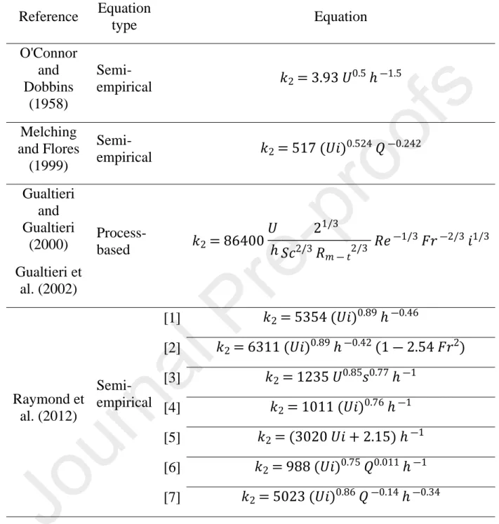
Table 2. Predictive equations considered in this study. All formulas were converted
into the reaeration rate coefficient k2 (d-1).
Reference Equation type Equation O'Connor and Dobbins (1958) Semi-empirical 𝑘2= 3.93 𝑈 0.5 ℎ―1.5 Melching and Flores (1999) Semi-empirical 𝑘2= 517 (𝑈𝑖) 0.524 𝑄―0.242 Gualtieri and Gualtieri (2000) Gualtieri et al. (2002) Process-based 𝑘2= 86400 𝑈 ℎ 21/3 𝑆𝑐2/3 𝑅𝑚 ― 𝑡2/3 𝑅𝑒―1/3 𝐹𝑟―2/3 𝑖1/3 [1] 𝑘2= 5354 (𝑈𝑖)0.89 ℎ―0.46 [2] 𝑘2= 6311 (𝑈𝑖)0.89 ℎ―0.42 (1 ― 2.54 𝐹𝑟2) [3] 𝑘2= 1235 𝑈0.85𝑠0.77 ℎ―1 [4] 𝑘2= 1011 (𝑈𝑖)0.76 ℎ―1 [5] 𝑘2= (3020 𝑈𝑖 + 2.15) ℎ―1 [6] 𝑘2= 988 (𝑈𝑖)0.75 𝑄0.011 ℎ―1 Raymond et al. (2012) Semi-empirical [7] 𝑘2= 5023 (𝑈𝑖)0.86 𝑄―0.14 ℎ―0.34
314 To compare measured gas exchange rate coefficients with gas exchange rate
315 coefficients obtained using predictive equations, the hydraulic parameters of each
317 evaluated at the reach scale and local parameters were evaluated for each sub-reach.
318 Stream discharge was calculated using a NaCl slug injection. Velocity was measured
319 using a field velocimeter (FP111 Global Water Flow Probe). The slope was derived
320 from the altitude gradient between upper and lower reach ends. Depth was measured
322 2.6. Reactive gases
323 In conjunction with helium, O2 and CO2 were measured by CF-MIMS at several 324 distances from the injection site. Measurements were externally calibrated using
325 micro-gas chromatograph (µGC) measurements, in the same way as for helium. In
326 both streams, the helium enrichment due to the injection was less than 1 µmol L-1, 327 so it did not induce significant degassing of O2 or CO2. In stream B, O2 and CO2 328 measurements failed because of a calibration error of the µGC.
329 CO2 evasion was calculated using the measured CO2 concentrations and the gas 330 exchange rate coefficient derived from the helium injection. Gas exchange rate 331 coefficients were first converted from He to CO2 based on the ratio of their Schmidt 332 numbers (equation 4). The Schmidt number for CO2 is given in table 1. The CO2 333 evasion rate at the stream-atmosphere interface (mol m-2 s-1) was then calculated 334 using the flux equation first developed for reaeration by Young and Huryn (1998)
335 and later derived for CO2 evasion (Billett et al. 2004; Hope et al. 2001; Öquist et al. 336 2009; Wallin et al. 2011) :
𝐶𝑂2 𝑒𝑣𝑎𝑠𝑖𝑜𝑛= (𝐶𝑂2 𝑠𝑡𝑟𝑒𝑎𝑚 ― 𝐶𝑂2 𝑒𝑞) × 𝑘𝐶𝑂2×
𝑄
337 where CO2 stream is the measured CO2 concentration (mol L-1), CO2 eq is the 338 concentration at equilibrium with the atmosphere (mol L-1), k
CO2 is the gas exchange 339 rate coefficient for CO2(s-1), Q is the stream discharge (L s-1), U is the mean velocity 340 of the water (m s-1) and w is the stream width (m).
341 2.7. List of the parameters
342 The parameters used in the paper are listed in table 3.
Table 3. List of parameters used in the paper.
Symbol Variable Unit
CCl concentration of chloride mol L-1
𝐶𝑑𝑜𝑤𝑛𝐶𝑙 downstream concentration of chloride mol L-1
𝐶𝑢𝑝𝐶𝑙 upstream concentration of chloride mol L-1
CHe concentration of helium mol L-1
𝐶𝑒𝑞𝐻𝑒 concentration of helium
at equilibrium with the atmosphere mol L
-1
𝐶𝑑𝑜𝑤𝑛𝐻𝑒 downstream concentration of helium mol L-1
𝐶𝑢𝑝𝐻𝑒 upstream concentration of helium mol L-1
Dx longitudinal dispersion coefficient m2 s-1
E Aeration efficiency []
Fr Froude number []
g standard acceleration due to gravity m s-2
h water depth m
i slope []
k gas exchange rate coefficient s-1
k2
gas exchange rate coefficient for O2 at
20°C
(also called reaeration rate coefficient)
kHe
gas exchange rate coefficient for He
at the stream temperature s
-1
L stream length m
Q stream discharge m3 s-1
Re Reynolds number []
Rm-t
mass transfer Reynolds number
(fitted with data) []
ScCO2 Schmidt number for CO2 []
ScHe Schmidt number for He []
ScO2 Schmidt number for O2 []
T stream temperature °C
t time s
U Stream velocity m s-1
x Distance m
w Stream width m
Dimensionless gas exchange factor []
ν kinematic viscosity m2 s-1
343 3. RESULTS
344 3.1. Gas exchange mapping
345 In both streams (A and B), measurements at several distances from the injection
346 site show a decrease in helium concentrations from upstream to downstream
347 (figure 3). In stream A, the helium concentrations decrease from 140 nmol L-1 at 348 14 m from the injection site to 84 nmol L-1 at 52 m downstream. A light rain event 349 occurred at the end of the experiment, just before the pump was set up at the most
350 upstream measurement location (9 m). The rain increased the gas exchanges at the
352 nmol L-1) than at 14 m (140 nmol L-1). In stream B, helium concentrations decrease 353 from 820 nmol L-1 at 15 m from the injection site to 650 nmol L-1 at 98 m
354 downstream. The CF-MIMS semi-continuous measurements allowed visualization
355 and quantification of the uncertainty in helium concentration estimates. The relative
356 standard deviation (RSD) of the 60 to 70 measurements available at each distance
357 was comprised between 1.7 and 4.5% in stream A, and between 0.9 and 1.5% in
358 stream B, attesting the stability of helium concentrations at each location. The lower
359 RSD in stream B is probably due to the higher helium injection rate. The large
360 number of measurements allows to perform a trend analysis on each plateau. It 361 reveals the absence of systematic decrease or increase of the helium concentration
362 upon a plateau (Supplementary data, Table A.2). In stream A, 4 plateaus have a slight
363 increasing trend and 3 plateaus have a slight decreasing trend. In stream B, 3 plateaus
364 have a slight increasing trend and one plateau has a slight decreasing trend. This
365 suggest an overall stability of the injection rate. Electrical conductivity can be
366 considered as stable along the streams, since its variation from upstream to
367 downstream is lower than the instrumental relative standard deviation. EC stability
368 thus shows the absence of major groundwater inputs prone to modify the helium
369 signal. In stream A, where measurements of O2 and CO2 are available, the 370 consistency in the variations of He, O2 and CO2 further confirms the absence of 371 disturbance of the gas content by groundwater inputs. CO2 concentrations in 372 groundwater, as measured at a small spring located 20 meters upstream from the
374 Inputs of such concentrated groundwater along the studied reach would have
375 induced a sharp increase in CO2 concentrations in the stream. However, CO2 376 concentrations follow a general decreasing trend, from at 299 µmol L-1 at 14 m to 377 288 µmol L-1 at 52 m, suggesting that there are no major inputs of groundwater along 378 the studied reach. Salt injections had to be stopped before the end of the experiments
379 because of a deficit in salt injection solution. It is unlikely to bias the conclusions
380 reached here, as EC does not change between the downstream and upstream ends of
Figure 3. Monitoring of helium in stream A (up) and B (down). Blue lines represent
the calibrated helium concentration, orange lines represent the electrical conductivity. Each plateau, highlighted by a yellow band, corresponds to a measurement location. Salt injection was stopped at 14:20 in stream A and at 16:40 in stream B. In stream A, it rained at the end of the experiment, when the pump was at 9 m from the injection site. Rain increased gas exchanges between stream and atmosphere thus lowering helium concentrations. The complete helium time series, including the measurements during the changes of measurement location, are presented in the Supplementary data, Figure A.2.
382 Global gas exchange rate coefficients in each stream were calculated using the
383 concentration difference between the most upstream and downstream locations
384 (equation 3). Since EC does not vary along each stream, the ratio between upstream
385 and downstream chloride concentrations is equal to 1 and can be simplified in
386 equation 3. The gas exchange rate coefficient for helium, kHe, was 196 d-1 in stream 387 A and 99 d-1 in stream B, corresponding to a reaeration rate coefficient, k
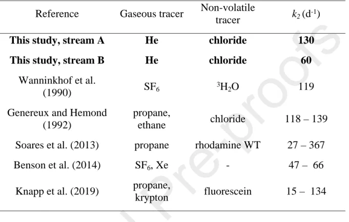
2, of 388 respectively 130 d-1 and 60 d-1 (equation 4). These k
2 are in the range of values found 389 by other gas tracer release experiments in headwater streams (table 4). The
390 reaeration rate coefficient is significantly higher in the 1st order stream (A) than in 391 the 2nd order stream (B). It is consistent with the observations of Wallin et al. (2011) 392 showing an increase in the rate of CO2 degassing with lower stream order.
Table 4. Reaeration rate coefficients measured in this study are in the range of
reaeration rate coefficients from other gas tracer release experiments performed in headwater streams (Q < 100 L s-1).
Reference Gaseous tracer Non-volatile
tracer k2 (d
-1)
This study, stream A He chloride 130
This study, stream B He chloride 60
Wanninkhof et al.
(1990) SF6
3H
2O 119
Genereux and Hemond (1992)
propane,
ethane chloride 118 – 139
Soares et al. (2013) propane rhodamine WT 27 – 367
Benson et al. (2014) SF6, Xe - 47 – 66
Knapp et al. (2019) propane,
krypton fluorescein 15 – 134
393 For each sub-reach, reaeration rate coefficients were calculated in the same way as
394 for the full stream reaches. Helium concentrations and reaeration rate coefficients 395 were then reported as a function of the distance from injection site (figure 4).
396 Uncertainties in the helium concentrations were estimated by the standard deviations
397 of the 60 to 70 CF-MIMS measurements available for each plateau. Standard
398 deviations are small (figure 4), demonstrating the robustness of the measurements.
399 Uncertainties in the gas exchange rate coefficients were estimated by randomly
400 subsampling each plateau of helium concentration. The gas exchange rate coefficient
402 randomly chosen value of the downstream plateau. The random sampling was
403 reiterated 1000 times for each sub-reach, leading to 1000 k2 values. The standard 404 deviation of the 1000 k2 values indicated the uncertainty due to helium measurement 405 (figure 4). The uncertainty is smaller in stream B than in stream A, due to the lower
406 noise level in stream B. A big advantage of the continuous measurements with
in-407 situ CF-MIMS is that it produces a significant number of measurements, which
408 allows to visualize and quantify the uncertainties. For the sub-reaches where EC was
409 available, the uncertainty due to EC measurements was quantified in the same way,
410 by sub-sampling EC values from each plateau. Taking into account the uncertainty 411 due to EC measurements increased the standard deviation by 50% in sub-reach A5, 412 by 8% in sub-reach A6 and by 10% in sub-reach B3. Thus, the uncertainty due to EC 413 measurements is lower than the uncertainty due to helium measurements, but is not
414 negligible. When possible, we recommend using a fluorescent dye as conservative
415 tracer, rather than NaCl. The measurement accuracy of fluorescent dyes is usually
416 higher, and florescent dyes are not present naturally in water, which lowers the
417 overall uncertainty on gas exchange rate coefficients.
418 The gas exchanges are heterogeneously distributed along the streams. In stream A,
419 k2 increases by a factor of 6 from the less turbulent zones (k2(A2) = 50 d-1;
420 k2(A4) = 70 d-1) to the highest cascade (k2(A5) = 360 d-1). Intermediary values are
421 found in the sub-reach displaying three successive small cascades (k2(A3) = 220 d-1) 422 and in the agitated sub-reach with no identifiable cascade (k2(A6) = 140 d-1). Thus, 423 reaeration rate coefficients are ranked according to the level of turbulence. In stream
424 B, the range of reaeration rate coefficients is larger. The reaeration rate coefficient
425 is 40 times higher in the cascade (k2(B3)= 1030 d-1) than in the flat area 426 (k2(B1) = k2(B2) = 25 d-1). Note that the first two sub-reaches B1 and B2, presenting 427 visually the same morphological characteristics, have the same k2 values, which 428 supports the reliability of the method. This mapping of gas exchanges evidences a
429 high heterogeneity of degassing along the streams. Exchanges are strongly focused
430 in cascades: a 35 cm high cascade loses as much gas as an 80 m long low-turbulent
Figure 4. Helium loss along stream A (top) and stream B (bottom) as a function of
the distance from the injection site. Helium concentrations were calculated at each location as the average of the plateau highlighted in figure 3. In stream A, it rained at the end of the injection, inducing higher gas exchanges between stream and atmosphere that lowered helium concentrations measured at 9 m from injection site. Error bars in the helium concentration represent ± σ. On top of each graph, reaeration rate coefficients are given (k2). The confidence intervals of the reaeration rate
coefficient, determined by a subsampling of each plateau of helium concentration, represent ± σ.
432 3.2. Suitability of predictive equations
433 The ten predictive equations given in table 2 were applied to the streams A and B
434 using the hydraulic parameters given in table A.1. At the reach scale, the ten
435 predictive equations systematically underestimate reaeration rate coefficients, by a
436 factor comprised between 1.2 and 2.2 (figure 5). Reaeration rate coefficients were
437 also calculated for each sub-reach using the local hydraulic parameters. The mean
438 and standard deviation of the ten predicted k2 values (obtained with the ten equations 439 of table 2) are given in table 5. On average, predictive equations strongly
440 underestimate gas exchanges in the cascade sub-reaches, while they are consistent
441 in low-turbulent zones. The spread of the k2 values given by the different equations, 442 indicated by their standard deviation, is also significantly higher in cascades than in
444 in cascades are due to the fact that physically, predictive equations are non-reliable
445 in high-turbulent zones (section 2.5). They are based on parameters that are highly
446 difficult to measure in cascades such as the stream depth. The underestimation of
447 predicted reaeration rate coefficients in cascades significantly biases the predictions
448 at the full-reach scale, leading to a systematic underestimation of global gas
449 exchanges.
Figure 5. Predictive equations systematically underestimate the reaeration rate
Table 5. Comparison of predicted and measured reaeration rate coefficients in each
sub-reach. The mean and standard deviation of the predicted k2 derive from the
statistics of the values obtained with the ten equations of table 2. Strea m Sub-reach Agitation level Measured k2 (d-1) Mean of the predicted k2 (d -1) Standard deviation of the predicted k2 (d-1) A2 calm 50 47 8 A3 cascade 220 111 38 A4 calm 70 61 13 A5 cascade 360 189 81 A A6 intermedia te 140 86 26 B1 calm 25 22 3 B2 calm 25 22 3 B B3 cascade 1030 679 441
450 3.3. Impacts on reactive gases
451 With a mean concentration of around 290 µmol L-1, stream A is oversaturated in 452 CO2, in the sense that it contains 10 times more CO2 than it would at equilibrium 453 with the atmosphere (figure 6). CO2 oversaturation is frequent in headwater streams, 454 because of inputs of groundwater that are highly concentrated in CO2 due to the 455 aerobic degradation of organic matter (Cole et al. 2007). Water-rock interaction can
456 also be a source of CO2 in streams, especially in karst regions (Chen et al. 2004). 457 The large excess of CO2 in stream A originates from a small spring that flows 20 458 meters upstream from the injection site. The spring water has a CO2 concentration
459 reaching 650 µmol L-1, which is 30 times higher than the atmospheric equilibrium. 460 Contrariwise, stream A shows an undersaturation in O2 (figure 6). Its O2 461 concentration is comprised between 280 and 300 µmol L-1, while at equilibrium with 462 the atmosphere it would be 344 µmol L-1. Undersaturation in O
2 is common in 463 headwater streams because they are mostly net heterotrophs (Knapp et al. 2015;
464 Riley and Dodds 2012; Young and Huryn 1999). In cascades, the state of the stream
465 is rapidly modified by strong exchanges of gas following partial pressure gradients.
466 CO2 oversaturation induces significant drops in CO2 in cascades, while O2 467 undersaturation induces gains in O2 (figure 6). Release of CO2 to the atmosphere, as 468 well as stream oxygenation, mainly occurs in the cascades. Note that the rain event
470 exchanges, leading to a drop in CO2 concentration and an increase in O2 471 concentration.
Figure 6. Cascades induce a rapid gain of O2 (red) and release of CO2 (black) along
stream A. Errors bars represent ± σ. Dashed lines indicate O2 (red) and CO2 (black)
equilibrium with the atmosphere. k2 values obtained by helium injection are recalled
on the top of the graph and area colors indicate the visually-determined level of turbulence.
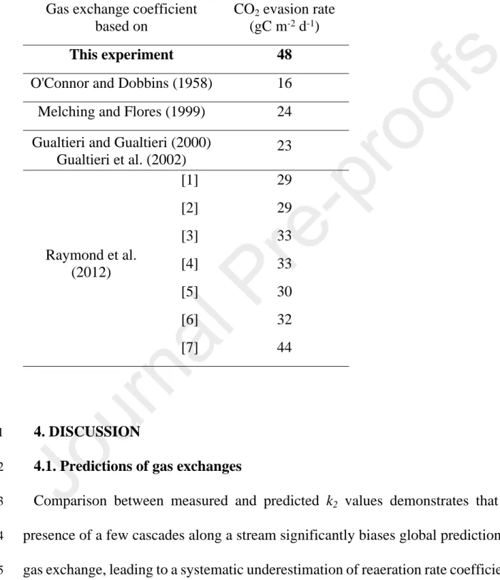
472 Based on the mean CO2 concentration of stream A and the gas exchange rate
473 coefficient measured with helium and converted to CO2 (equation 4), we estimated 474 the global CO2 evasion rate of stream A at 47 µmol m-2 s-1 (equation 6). This 475 corresponds to 48 gC m-2 d-1, which is close to the evasion rate of 56 gC m-2 d-1 that
476 was measured in a Canadian steep headwater stream by direct CO2 injections 477 (McDowell and Johnson 2018). The CO2 evasion rate of stream A was also 478 calculated using the gas exchange rate coefficients predicted by the empirical
479 equations of table 2. It yielded systematically lower CO2 evasion rates, comprised 480 between 16 and 44 gC m-2 d-1 (table 6). Thus, the underestimation of gas exchange 481 rate coefficients by empirical equations (section 3.2.) leads to a significant
482 underestimation of the CO2 flux from headwater streams.
483 If CO2 concentrations in the stream were modified solely by gas exchanges
484 with the atmosphere, the calculated evasion rate of 48 gC m-2 d-1 would imply a 485 decrease of 50 µmol L-1 in the CO
2 concentration between the upstream and the 486 downstream end of the reach A. This is higher than the measured net loss of CO2, 487 close to 20 µmol L-1 (Figure 6), showing that other processes, such as oxygenic 488 respiration, partly counterbalance the loss of CO2 to the atmosphere. It highlights 489 that the CO2 evasion rates cannot be derived directly from the changes in CO2 490 concentration along the streams.
Table 6. CO2 evasion rate in stream A derived from the gas exchange rate
coefficients obtained with the equations of table 2. Predictive equations of gas exchange rate coefficients lead to an underestimation of CO2 evasion rate.
Gas exchange coefficient based on
CO2 evasion rate
(gC m-2 d-1)
This experiment 48
O'Connor and Dobbins (1958) 16
Melching and Flores (1999) 24
Gualtieri and Gualtieri (2000) Gualtieri et al. (2002) 23 [1] 29 [2] 29 [3] 33 [4] 33 [5] 30 [6] 32 Raymond et al. (2012) [7] 44 491 4. DISCUSSION
492 4.1. Predictions of gas exchanges
493 Comparison between measured and predicted k2 values demonstrates that the 494 presence of a few cascades along a stream significantly biases global predictions of
495 gas exchange, leading to a systematic underestimation of reaeration rate coefficients.
497 that empirical models underestimate gas exchanges in high-channel slope streams.
498 McDowell and Johnson (2018) also highlighted, when studying a headwater stream,
499 that models underestimate gas exchange rate coefficients for high k values.
500 Processes governing gas exchanges in cascades fundamentally differ from those in
501 flowing sections (section 2.5). In cascades, air bubbles have a strong control over
502 gas exchanges (Chanson 1995; Chanson and Toombes 2002; Cirpka et al. 1993).
503 Overlooking specific processes occurring in cascades leads to an underestimation of
504 gas exchanges in headwater catchments, where shallow streams often display natural
505 cascades. Increasing the reliability of predictions would require separate 506 consideration of low-turbulent zones and cascades. For low-turbulent stream
507 sections, our study confirms the predictive capacities of the empirical and
semi-508 empirical equations of table 2. For cascades, predictions are more challenging and
509 require additional morphological characterization or field experiments. Studies
510 focused on spillways in flumes (Baylar et al. 2006; Essery et al. 1978; Gameson
511 1957; Gulliver et al. 1998; Khdhiri et al. 2014; Tebbutt 1972; Toombes and Chanson
512 2005)and on dams (Caplow et al. 2004; Gamlin et al. 2001) or cascades (Cirpka et
513 al. 1993) in rivers, use the aeration efficiency E instead of the gas exchange rate
514 coefficient k. Aeration efficiency was defined by Gameson (1957) and represents
515 the total change in gas concentration occurring in the cascade, normalized by the
air-516 water concentration gradient:
𝐸 =𝐶𝑑𝑜𝑤𝑛― 𝐶𝑢𝑝 𝐶𝑒𝑞― 𝐶𝑢𝑝
517 where Cup (mol L-1) is the upstream concentration, Cdown (mol L-1) is the 518 downstream concentration and Ceq (mol L-1) is the dissolved gas concentration at 519 equilibrium with the atmosphere. Equations derived from lab experiments predict
520 aeration efficiency as a function of cascade total height and, if applicable, of
521 additional morphological parameters of the cascade such as the height of
522 intermediate steps, or the angle of the weir (Baylar and Bagatur 2006; Baylar et al.
523 2006; Baylar et al. 2011; Essery et al. 1978; Khdhiri et al. 2014). The morphological
524 characteristics of the hydraulic structure seem to be more reliable to predict aeration
525 in cascades than the depth of the water layer. However, if these morphological 526 characteristics are well-defined in flumes, they are much harder to describe properly
527 in natural streams, where cascades are made up of heterogeneous stones and pieces
528 of wood. For more accurate gas exchange quantification, direct measurements
529 remain necessary in cascades.
530 4.2. Impact of cascades on groundwater discharge estimates
531 Groundwater discharge in streams is commonly quantified using the natural gas
532 tracer 222Rn. Some authors like Gilfedder et al. (2019) and Cartwright et al. (2014) 533 raised the question of the impact of the variability of turbulence on 222Rn degassing 534 rate and thus on groundwater discharge estimation. Our study points out that
535 cascades, by generating a fast equilibration between the stream and the atmosphere,
536 erase an important part of the gaseous groundwater signal in the stream (e.g. Rn, He,
537 Ar, CO2, CH4, N2, N2O). A cascade that is a few tens of centimeters high can lose as 538 much gas as a hundred meter long stream. Since such cascades are very common in
539 low-order streams, this is prone to yield an underestimation of the groundwater
540 discharge calculated by 222Rn mass balances. The location of the cascades should be 541 taken into account when defining the 222Rn sampling strategy and their number and 542 size between the up and down 222Rn sampling locations minimized. Our results 543 suggest that in reaches without notable cascades, one can reasonably calculate the
544 222Rn degassing rate with empirical equations. In reaches displaying notable
545 cascades, however, direct gas tracer experiments appear to be necessary.
546 4.3. Hot spots of reaeration
547 Studies based on flume experiments recommend the use of dams in rivers subject 548 to eutrophication to enhance water reaeration (Tebbutt 1972). Our study shows that
549 natural cascades significantly increase the oxygenation of headwater streams. In this
550 way, they might strongly help sustaining aerobic metabolism, and thus provide a
551 crucial ecosystem service in headwater catchment subject to eutrophication (Dodds
552 and Smith 2016; Garnier and Billen 2007). Considered as reaeration hot spots, small
553 cascades have the potential to enhance measurably the ecological conditions of
554 eutrophic streams and might thus be considered in management and restoration
555 strategies (Palmer et al. 2005).
556 4.4. Hot spots of CO2 emission
557 Most headwater streams are net sources of atmospheric CO2 (Cole et al. 2007; 558 Marx et al. 2017). Indeed, organic matter respiration occurring in the contributing
559 compartments (aquifer, hyporheic zone, soil) and in the stream network itself is often
561 equilibrium with the atmosphere. Drops in CO2 partial pressure in water after 562 cascades and highly turbulent zones have been evidenced in headwater
563 streams (Duvert et al. 2018; Leibowitz et al. 2017; Natchimuthu et al. 2017). In karst
564 systems, these drops have been linked to water softening (Chen et al. 2004). At a
565 much bigger scale, Liu et al. (2017) showed that CO2 outgassing from low-gradient 566 large rivers was strongly controlled by the geomorphology. Here, by simultaneously
567 mapping the loss of a gas tracer and the changes in CO2 concentration along a 568 headwater stream, we establish a direct link between streambed morphology, gas
569 exchanges, and CO2 release to the atmosphere. We show that cascades significantly 570 enhance gas exchanges, leading to a fast CO2 release to the atmosphere. In a study 571 focused on the temporal variability of gas exchanges, McDowell and Johnson (2018)
572 showed that 84% of CO2 emissions from a steep headwater stream occurred when 573 discharge was higher than the median. They suggested that high flow events, because
574 they increase turbulence, can be seen as “hot moments” of CO2 emission in 575 headwater streams (McClain et al. 2003). Here, we highlight the spatial variability
576 of CO2 emissions and show that similarly, by increasing gas exchanges, cascades 577 can be viewed as “hot spots” of CO2 emission in headwater streams.
578 If we assume the 19 km-long first order stream network of our 35 km2 catchment 579 has the same CO2 emission rate as the studied stream A, a rough estimate of the total 580 evasion of CO2 over all first-order streams of the catchment can be calculated. We 581 limit the upscaling to the first-order stream network of a small catchment, in which
583 stream A. Predictive equations from table 2 would lead to a total CO2 emission 584 comprised between 150 and 300 tC year-1 with the mean of the outputs from the ten 585 equations being 220 tC year-1, while the measured gas exchange rate leads to a CO
2
586 emission of 330 tC year-1. Such a rough, first-order estimation indicates that the 587 prediction of gas exchange rate coefficients at a large-scale with empirical equations
588 is likely to induce a general underestimation of CO2 emission from headwater 589 catchments. Similarly, empirical equations probably lead to an underestimation of
590 the emission of other greenhouse gases such as CH4.
591 5. CONCLUSION
592 Using continuous helium injection, we mapped gas exchanges along two low-slope
593 headwater streams in a temperate catchment in Brittany (France). Our experimental
594 set-up took advantage of the real-time data visualization allowed by the in-situ
CF-595 MIMS. It highlights the new opportunities offered by this technology, in terms of
596 spatial as well as temporal characterization of gas exchange processes. The
semi-597 continuous measurements allow to visualize and to quantify the uncertainties.
598 We evidenced a high spatial variability of gas exchanges, related to the small-scale
599 heterogeneity of the streambed morphology, which is a characteristic feature of
600 headwater streams. During one of our tracer tests, a small cascade was responsible
601 for almost half of the helium loss, while it occupied less than 4% of the total stream
602 length. Nevertheless, the equations predicting the gas exchange rate coefficients in
604 exchanges in natural cascades. As a result, while empirical relationships perform
605 well in low-turbulent zones, they systematically underestimate gas exchange rate
606 coefficients as soon as small cascades are present. This highlights the necessity of
607 performing direct measurements of gas exchange rate coefficients in reaches
608 displaying cascades while low-turbulent zones can be efficiently characterized by
609 empirical equations.
610 Additional CO2 and O2 measurements highlighted that small cascades strongly 611 modify the chemical state of headwater streams. High gas exchange rate coefficients
612 allow a fast incorporation of O2 in the water and a fast release of CO2 to the 613 atmosphere. Thus, cascades sustain respiration by rebalancing O2 concentrations in 614 the stream. At the same time, they promote the evasion of the oversaturated CO2 to 615 the atmosphere. Finally, small natural cascades are hot spots for both stream
616 oxygenation and greenhouse gas emission. Rough calculations of CO2 emissions 617 showed that the use of empirical equations leads to an underestimation of global CO2
618 emissions from headwater streams. Since the small-scale morphological
619 heterogeneity is a characteristic feature of headwater streams, the upscaling effort
620 could be helped by a distinct consideration of cascades and low-turbulent sections.
621 The first step would be to separately characterize gas exchange processes in these
622 totally different hydrodynamic regimes. The second step would be to estimate the
623 proportion of these two regimes in the stream network. This could be helped by
624 innovative technologies such as LIDAR, allowing a fine-scale characterization of
626 ACKNOLEDGMENTS
627 PhD of Camille Vautier is funded by the French Ministry for Higher Education,
628 Research and Innovation. Most of the equipment, especially the CF-MIMS, was
629 funded by the CRITEX project (ANR-11-EQPX-0011). Analysis with µGC were
630 performed within the CONDATE-EAU analytical platform in Rennes. Field work
631 was performed in the Long‐Term Socio‐Ecological Research (LTSER) site “Zone
632 Atelier Armorique”. The authors thank Christophe Petton and Virginie Vergnaud for
633 their precious involvement in the field experiments and in the laboratory analysis.
634 We also greatly thank Madeleine Nicolas for the proof-reading of the manuscript.
635 We thank the four reviewers, including Jordan F. Clark, for constructive comments
636 and suggestions.
APPENDIX A: supplementary data
637 - Figure A.1: Photograph of the bubbling system
638 - Figure A.2: Entire time series of the monitoring of helium
639 - Table A.1: Hydraulic and morphologic characteristics of reaches A and B 640 - Table A.2: Test of the stability of the plateaus of helium concentration
641 REFERENCES
642 Aristegi, L., O. Izagirre & A. Elosegi, 2009. Comparison of several methods to
643 calculate reaeration in streams, and their effects on estimation of metabolism.
644 Hydrobiologia 635(1):113-124 doi:10.1007/s10750-009-9904-8.
645 Avery, E., R. Bibby, A. Visser, B. Esser & J. Moran, 2018. Quantification of
646 Groundwater Discharge in a Subalpine Stream Using Radon-222. Water 10(2)
647 doi:10.3390/w10020100.
648 Baird, M. H. I. & J. F. Davidson, 1962. Annular jets—II: Gas absorption. Chemical
649 Engineering Science 17(6):473-480
doi:https://doi.org/10.1016/0009-650 2509(62)85016-7.
651 Baylar, A. & T. Bagatur, 2006. Experimental studies on air entrainment and oxygen
652 content downstream of sharp-crested weirs. Water and Environment Journal
653 20(4):210-216 doi:10.1111/j.1747-6593.2005.00002.x.
654 Baylar, A., M. E. Emiroglu & T. Bagatur, 2006. An experimental investigation of
655 aeration performance in stepped spillways. Water and Environment Journal
656 20(1):35-42 doi:10.1111/j.1747-6593.2005.00009.x.
657 Baylar, A., M. Unsal & F. Ozkan, 2011. GEP modeling of oxygen transfer efficiency
658 prediction in aeration cascades. KSCE Journal of Civil Engineering
659 15(5):799-804 doi:10.1007/s12205-011-1282-x.
660 Benson, A., M. Zane, T. Becker, A. Visser, S. Uriostegui, E. DeRubeis, J. Moran,
661 B. Esser & J. Clark, 2014. Quantifying Reaeration Rates in Alpine Streams
662 Using Deliberate Gas Tracer Experiments. Water 6(4):1013-1027
663 doi:10.3390/w6041013.
664 Bernot, M. J., D. J. Sobota, R. O. Hall Jr, P. J. Mulholland, W. K. Dodds, J. R.
665 Webster, J. L. Tank, L. R. Ashkenas, L. W. Cooper, C. N. Dahm, S. V.
666 Gregory, N. B. Grimm, S. K. Hamilton, S. L. Johnson, W. H. Mcdowell, J. L.
667 Meyer, B. Peterson, G. C. Poole, H. M. Valett, C. Arango, J. J. Beaulieu, A.
668 J. Burgin, C. Crenshaw, A. M. Helton, L. Johnson, J. Merriam, B. R.
669 Niederlehner, J. M. O’brien, J. D. Potter, R. W. Sheibley, S. M. Thomas & K.
670 Wilson, 2010. Inter-regional comparison of land-use effects on stream
671 metabolism. Freshwater Biology 55(9):1874-1890
doi:doi:10.1111/j.1365-672 2427.2010.02422.x.
673 Billett, M. F., S. M. Palmer, D. Hope, C. Deacon, R. Storeton-West, K. J.
674 Hargreaves, C. Flechard & D. Fowler, 2004. Linking land-atmosphere-stream
675 carbon fluxes in a lowland peatland system. Global Biogeochemical Cycles
676 18(1) doi:10.1029/2003gb002058.
677 Bishop, K., I. Buffam, M. Erlandsson, J. Fölster, H. Laudon, J. Seibert & J.
678 Temnerud, 2008. Aqua Incognita: the unknown headwaters. Hydrological