Control of agricultural nonpoint source pollution in Kranji Catchment, Singapore

(1)

Control of Agricultural Nonpoint Source Pollution in

Kranji Catchment, Singapore

by

Margaret A. Hoff

B.S.E. Civil and Environmental Engineering Duke University, 2010

Submitted to the Department of Civil and Environmental Engineering in Partial Fulfillment of the Requirements for the Degree of

MASTER OF ENGINEERING in Civil and Environmental Engineering

at the

Massachusetts Institute of Technology June 2013

Signature of Author _____________________________________________________________ Margaret A. Hoff Department of Civil and Environmental Engineering May 10, 2013 Certified by____________________________________________________________________ Peter Shanahan Senior Lecturer of Civil and Environmental Engineering Thesis Supervisor Accepted by ___________________________________________________________________

Heidi M. Nepf Chair, Departmental Committee for Graduate Students

(2)

(3)

3

Control of Agricultural Nonpoint Source Pollution in Kranji Catchment, Singapore

by

Margaret A. Hoff

Submitted to the Department of Civil and Environmental Engineering on May 10, 2013 in Partial Fulfillment of the Requirements for the Degree of

Master of Engineering in Civil and Environmental Engineering

Abstract

Singapore’s Kranji Reservoir is highly sensitive to nutrient and bacterial pollution, both of which can be directly traced to agricultural runoff. Water quality samples were collected along the main drainage channel in the Neo Tiew subcatchment, which drains to Kranji Reservoir, in an effort to determine the source and degree of agricultural nonpoint source pollution in the area. Grab samples collected from eight sampling locations along the reach of the drainage channel under wet- and dry-weather conditions were analyzed for nitrogen, phosphorus, and bacterial species, as well as total suspended solids. High nutrient and bacterial concentrations were observed at sampling locations in the upstream region of the subcatchment, with total nitrogen as high as 19.8 mg/L, total phosphorus as high as 2.12 mg/L, and a peak total coliform count over 1,000,000 MPN/100 mL. The peak concentration of most of the observed contaminants occurred directly downstream from an intensive row-cropping vegetable production operation. These observations indicate that this farming operation is a primary, though not sole, contributor to nonpoint source pollution in the area. A constructed free-water-surface treatment wetland was designed to treat runoff immediately downstream from the identified source. The designed wetland is projected to remove, depending on flow conditions, between 13 and 99% of influent total phosphorus, 51 to 99% of influent total nitrogen, greater than 99% of influent fecal coliform, and approximately 75% of influent total suspended solids. Agricultural management practices for mitigating runoff contamination are also recommended, including cyclic irrigation and crop rearrangement. It is evident that agricultural nonpoint source pollution is a significant water quality concern in the Neo Tiew subcatchment in particular and the Kranji catchment in general, but there are a number of promising and practical options to address this problem.

Thesis Supervisor: Peter Shanahan

(4)

(5)

5

Acknowledgments

Innumerable thanks to Peter Shanahan for his guidance, insight, and good humor throughout this project.

Thanks to Ndeye Awa Diagne, Tsung Hwa Sophia Burkhart, and Halle Ritter for their help in the fieldwork and laboratory portions of this study.

Many thanks to Le Song Ha, Syed Alwi Bin Sheikh Bin Hussien Alkaff, Eveline Ekklesia, Professor Chua Hock Chye Lloyd, and others at Nanyang Technological University for their assistance and contributions to this work while in Singapore and beyond.

(6)

(7)

7

List of Figures

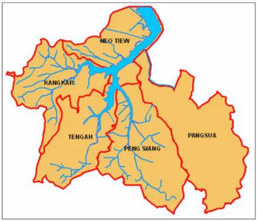
Figure 1: Map of Kranji catchment and subcatchments (NTU 2008) ... 16

Figure 2: Neo Tiew subcatchment sampling location (Le 2013) ... 16

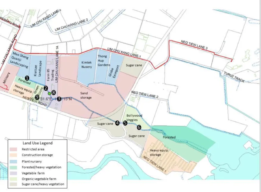
Figure 3: Map of land use and sampling locations in Neo Tiew subcatchment. ... 23

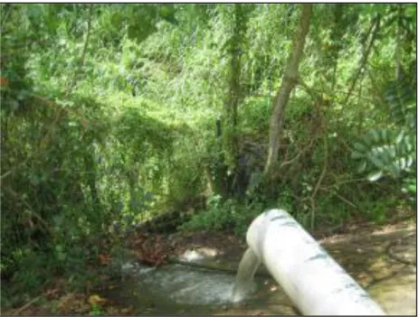
Figure 4: Sampling location 1. ... 24

Figure 12: Bucket collection equipment at sampling location 6. ... 29

Figure 13: Supercritical flow region at sampling location 2 with overlaid trapezoid. ... 30

Figure 14: Supercritical flow region at sampling location 8 with overlaid arc. ... 30

Figure 15: Nitrate samples prepared for colorimetric analysis using CHEMetrics method. ... 32

Figure 16: Total coliform presence in Quanti-Tray/2000. Yellow wells are positive for total coliform. ... 34

Figure 17: Enterococci presence in Quanti-Tray/2000. Blue fluorescent wells are positive for enterococci. ... 34

Figure 18: Nitrogen concentrations on 1/16/13. ... 36

Figure 19: Nitrogen concentrations on 1/22/13. ... 37

Figure 20: Phosphorus concentrations on 1/16/13. ... 37

Figure 21: Phosphorus concentrations on 1/22/13. ... 38

Figure 22: Nitrogen concentrations with additional points, 1/16/13. ... 39

Figure 23: Nitrogen concentrations with additional points, 1/22/13. ... 39

Figure 24: Phosphorus concentrations with additional points, 1/16/13. ... 40

Figure 25: Phosphorus concentrations with additional points, 1/22/13. ... 40

Figure 26: Bacterial counts on 1/16/13. ... 42

Figure 27: Bacterial counts on 1/22/13. ... 42

Figure 28: Bacterial counts with additional points, 1/16/13. ... 43

Figure 29: Bacterial counts with additional points, 1/22/13. ... 43

Figure 30: Total suspended solids, 1/16/13. ... 44

Figure 31: Total suspended solids, 1/22/13. ... 44

Figure 32: Comparison of observed contaminant concentrations to Le (2013). ... 48

Figure 33: Subcatchment area from Le (2013). ... 58

Figure 34: Subcatchment area contributing runoff to sampling location 3. ... 59

Figure 35: Singapore IDF curve (PUB 2011). ... 60

Figure 36: Proposed wetland location... 66

Figure 37: Wetland design, plan view. ... 69

Figure 38: Wetland design, profile view... 69

Figure 39: Drainage channel cross-section (Le 2013). ... 70

Figure 40: Drainage channel flashboard design, downstream side... 71

(10)

10

Figure D-1: Wetland design with dimensions, profile view. ... 88 Figure D-2: Wetland design with dimensions, plan view. ... 89 Figure D-3: Channel flashboard design with dimensions, downstream view. ... 90

(11)

11

List of Tables

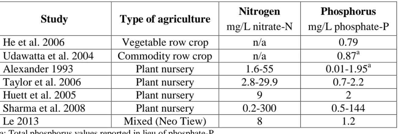
Table 1: Typical values of nitrogen and phosphorus concentrations in agricultural runoff. ... 20

Table 2: Calculated channel flow at locations 2 and 8. ... 31

Table 3: Range of observed nutrient concentrations... 35

Table 4: Range of measured bacteria concentrations. ... 41

Table 5: Field blank analysis results, 1/16/13 and 1/22/13. ... 45

Table 6: Duplicate sample analysis results. ... 46

Table 7: Comparison of design parameters to studied wetlands. ... 61

Table 8: Projected average wetland treatment performance. ... 75

Table A-1: Sampling location information. ... 83

(12)

(13)

13

1. Introduction

1.1 Singapore Water Management

This section was written collaboratively with Ndeye Awa Diagne.

Singapore is lauded by many, including the World Health Organization, as an archetype of an integrated water resources management model (Chen et al. 2011). This recognition is not because the small city-state has abundant water. On the contrary, it lacks sufficient naturally occurring water resources to sustain its population of 4.8 million. Water limitations are serious enough to warrant Singapore’s inclusion by the United Nations on its list of water-scarce countries (Ong 2010). Though the average annual rainfall of 2,400 mm is above the global average, the country lacks the land area necessary to harvest an adequate amount of that precipitation (Tan et al. 2009). Furthermore, the small island has no other sources of renewable freshwater, lacking the volumes of surface- and groundwater that typically sustain other countries. The thirsty country, which currently consumes approximately 1.36 billion liters of water per day (Tortajada 2006), is projected to continue to grow, reaching a population of 6.5 million in the next 50 years (Chen et al. 2011), further stressing its already scarce water resources.

Singapore scores remarkably high on a measure of the proportion of the population with adequate water supply, both in terms of quantity and quality. As Chen et al. (2011) report, 100% of the population has consistent access to water of sufficient quantity to meet their consumption demands. Furthermore, 99.96% or higher of that water supply meets the World Health Organization (WHO) drinking water standard, which, though not a universal standard, is generally considered sufficient to ensure potability of water. Similarly, 100% of the population is reported to have access to “adequate sanitation” (Chen et al. 2011). The country’s impressive performance in light of water scarcity is the result of careful management by Singapore’s national water utility, the Public Utilities Board (PUB), of the country’s four “National Taps,” its four sources of water (Tan et al. 2009).

As previously mentioned, Singapore gets an above-average amount of rainfall, but the country simply is not physically large enough to collect enough of that water as it falls. This spatial limitation has long been the target of engineering projects in Singapore and has resulted in an intricate network of rainwater collection channels and reservoirs, considered the country’s first National Tap (Tan et al. 2009). The rainwater collection system provides about 50% (Chen et al. 2011) of Singapore’s daily water consumption of 1.36 billion liters (Tortajada 2006). Efforts to expand the ability to harvest precipitation are continuing, including progressive rooftop harvesting schemes and continuous expansion of the reservoir network, with the aim of transforming 90% of Singapore’s land area into water catchment. Despite the advanced technology and the government’s aggressive expansion of rainwater collection systems, physical limitations still necessitate other sources of water to meet the country’s needs (Tan et al. 2009). Singapore’s second National Tap is imported water from Johor, Malaysia, which makes up another 40% of its water supply (Chen et al. 2011). Singapore has imported a large percentage of

(14)

14

its water since it separated from the Federation of Malaysian States in 1965, but the relationship has often been tense and uncertain in the intervening years. At various times, Malaysia has threatened to cut off the water supply for political or economic reasons and agreement on pricing has been a long-standing issue (Chen et al. 2011). There is currently an agreement in place that will provide water to Singapore through 2061 at a price of less than S$0.01 per 1,000 liters, but further terms are uncertain (Tortajada 2006). Driven by at-times acrimonious relations with Malaysia, Singapore has investigated other international sources for water, including Indonesia, but has been deterred by high development costs and the inherent insecurity of relying on other nations for natural resources (Chen et al. 2011). Most recently, Singapore has invested significant financial and political resources into careful water resource management, as well as the development of its third and fourth National Taps, desalination of seawater and reuse of wastewater, with the ultimate goal of national water independence (Tortajada 2006).

The country’s first large desalination plant, the Tuas Desalination Plant, opened in 2005 with a price tag of S$200 million (Chen et al. 2011). Though desalination technology is improving rapidly, it still has relatively low capacity and is highly energy intensive. Accordingly, the Tuas plant can supply 113 million liters per day (less than 7% of the country’s current water demand) at a cost of S$0.78 per 1,000 liters (Tortajada 2006). For a sense of the economics, this water source is more than seventy times more expensive than imported water, but, as of 2011, was still the lowest cost seawater desalination plant in the world (Chen et al. 2011). High costs and lagging technology in desalination have encouraged Singapore to explore water reuse technology, which typically has lower economic costs than desalination but higher social barriers.

Reuse of highly treated wastewater has been explored as an alternative water source in Singapore since 1972, with the first operational treatment plant built in 2000 (Tortajada 2006). The recycled waste stream and fourth National Tap, locally termed “NEWater,” is currently produced at four facilities across the country and will ultimately account for more than 30% of the national water supply (Chen et al. 2011). Though treated to a higher level than necessary to meet standards for human consumption, the majority of NEWater is currently used for industrial water needs rather than domestic (potable) distribution. Since 2003, a small percentage of the recycled water has been designated for indirect potable use, in which the highly treated effluent is mixed into existing raw water sources (Ching 2010). The percentage of NEWater designated for indirect potable use is expected to rise, but will still remain much lower than industrial usages (Tortajada 2006). Just as with desalination, production costs will likely drop as the technology evolves, but current reuse treatment costs are already low at approximately S$0.30 per 1,000 liters, which is less than half the cost of desalination (Tortajada 2006).

Singapore’s success in water provision, particularly in the arena of water reuse, has largely been attributed to the organization of its water management institution, the Public Utilities Board. Since 2001, PUB has managed the entire water cycle within the country, including potable water delivery, sewage, waste treatment, and rainwater collection (Tan et al. 2009). In addition to controlling the entire water cycle, PUB was also given general autonomy over its functions, which has allowed the agency unilateral authority over all aspects of water governance, including pricing structures, regulatory frameworks, and enforcement mechanisms (Tortajada 2006). This structure is touted by many to “eliminate administrative barriers in water management and make implementation effective and efficient” (Chen et al. 2011). Furthermore, PUB is widely

(15)

15

considered to effectively include the private sector when appropriate and foster public acceptance and political will through its success (Tortajada 2006).

In 2006, PUB launched the Active Beautiful Clean Waters (ABC Waters) Programme, a strategic initiative to open Singapore’s reservoirs and waterways to the public for recreational activities. The larger objective of the ABC Waters Programme is to make Singaporeans cherish their water bodies and be more conscious of water scarcity (PUB 2009). The recreational activities include kayaking, fishing, barbecue, and picnic activities, and may involve direct contact with the water bodies. However, water quality of the reservoirs and waterways has been a concern for PUB. In fact, recent studies have reported contamination in the nation’s water reservoirs and the stormwater drains feeding them. Both urban and agricultural runoff has been reported to contain high levels of pollutants including suspended solids, nutrients, heavy metals, and pathogenic bacteria (Wang 2012). In order to protect public health, there have been ongoing studies and investigations to evaluate the levels of contamination within reservoir catchments and bacteria loading to the reservoirs and waterways (Chua et al. 2010).

1.2 Kranji Reservoir Water Quality

Kranji Reservoir is a large drinking water reservoir in the northwestern region of Singapore and is surrounded by a wide variety of land uses, dominated by a mixture of agricultural activities. Historically, Kranji has been plagued by the same water quality issues as the rest of Singapore’s reservoirs and has had particularly high concentrations of nutrients and bacteria (NTU 2008). Agricultural nonpoint source pollution has been identified as a major contributor to the nutrient and bacteria contamination in Kranji Reservoir (NTU 2008). An investigation of storm-event-mean concentrations at a variety of locations in the Kranji watershed (Figure 1) has revealed a significant contribution from a sampling location in the Neo Tiew subcatchment (Le 2013). Specifically, in a study of wet-weather nonpoint-source runoff from around the Kranji catchment, samples collected in the Neo Tiew subcatchment at a location draining two plant nurseries and one vegetable farm (Figure 2) presented maximum event-mean concentrations of nitrogen, phosphorus, and total suspended solids (TSS). In the study, which included composite samples from 10 storm events in 2011, average event-mean concentration of total nitrogen at the Neo Tiew sampling point was 13.2 mg/L, total phosphorus was 3.2 mg/L, and TSS was 522 mg/L (Le 2013). These concentrations, as well as those of constituent chemical species of nitrogen and phosphorus, were the highest observed around the Kranji catchment by Le (2013).

(16)

16

Figure 1: Map of Kranji catchment and subcatchments (NTU 2008)

(17)

17

A 2008 study of water quality in the Kranji Reservoir by Nanyang Technological University evaluated bacteriological contamination at a sampling point in the Neo Tiew subcatchment near Le’s Neo Tiew sampling location (NTU 2008). The mean cell density of E. coli of 14 samples collected at the location was 4,560 Most Probable Number (MPN)/100 mL. The mean enterococci density was similarly high at 2,410 MPN/100 mL (NTU 2008). Additionally, past studies by Master of Engineering students from the Massachusetts Institute of Technology (MIT) have observed high levels of bacterial contamination in agricultural runoff in the Kranji catchment. E. coli density as high as 290,000 colony-forming units (CFU)/100mL was found in nonpoint source runoff in the Neo Tiew subcatchment (Dixon et al. 2009). Bossis (2011) observed very high concentrations of biological contamination indicators in agricultural runoff in the Kranji catchment. The highest observed values were 21,000,000 MPN/100 mL of fecal coliform (FC), 10,000,000 MPN/100 mL E. coli, and 370,000 MPN/100 mL enterococci, all of which were observed in areas draining plant nurseries. Though the samples were taken in a different subcatchment, the measured concentrations indicate the significant bacterial contamination that can be present in agricultural runoff (Bossis 2011).

Nutrient and bacteria contamination in Kranji is of concern for a number of reasons. First, Kranji is a phosphorus-limited environment in which inputs of phosphorus have been shown to cause blue-green algae blooms. This eutrophication, in addition to creating objectionable odor and aesthetic conditions, can lead to hypoxia of the reservoir environment upon decomposition (NTU 2008). Though nitrogen is not the limiting nutrient in the Kranji environment, water samples from the reservoir with elevated nitrogen levels have been shown to stimulate increased chlorophyll production relative to samples without elevated nitrogen inputs (NTU 2008). Lastly, the presence of total coliform, E. coli, and enterococci in surface water is indicative of human fecal bacteriological contamination. Human contact with microbial contamination in water can result in intestinal illness and death (Douglas-Mankin and Okoren 2011).

It is clear that in order for Kranji to meet the goals of the ABC Waters Programme, nitrogen, phosphorus, and bacterial contamination of the reservoir must be mitigated to the extent possible. As the agricultural operations in the Neo Tiew subcatchment have been identified as substantial contributors of these contaminants, a mitigation plan needs to be developed for this nonpoint source of pollution. Before a remedy can be prescribed, a determination must be made as to the primary source of these contaminants. The agricultural activities in the Neo Tiew subcatchment include containerized plant nurseries, organic fruit and vegetable production, and intensive row crop vegetable production. Additionally, there are non-agricultural activities in the subcatchment, including large-scale sand storage for concrete production, construction equipment storage, and military training. Once it is determined which land uses are driving the high pollutant concentrations in the Neo Tiew drainage channel, a solution can be devised. This study endeavors to determine the source of the bacteria and nutrient contamination observed in the Neo Tiew subcatchment and to propose pollution control solutions. The pollution control plan includes upstream source mitigation strategies and design of a downstream contaminant remediation system.

(18)

18

2. Nonpoint Source Pollution

Nonpoint source pollution is an increasing problem in surface waters around the world, with contributions from agriculture of particular concern. Different agricultural activities result in different contaminant profiles in runoff, but the primary constituent contaminants and treatment options share similarities across different agricultural industries (Novotny and Olem 1994). Most relevant for this study are explorations of runoff from plant nursery operations, intensive row crop farms, and organic produce cultivation, but studies of remediation of other high-intensity agricultural and landscaping activities with high fertilizer or nutrient application rates are applicable as well. There have been several studies aimed at understanding and categorizing the environmental consequences of runoff from the highly intensive types of agriculture employed in the Neo Tiew subcatchment. Additionally, some studies have built on that understanding, or similar studies regarding other types of agriculture, and explored Best Management Practices, or BMPs, that can be used to remediate contaminated agricultural runoff. Studies of BMPs can largely be divided into those addressing structural BMPs, such as treatment wetlands and vegetative filter strips, and those addressing non-structural BMPs, such as irrigation management and crop selection. The body of literature is largely applicable to the study of agricultural runoff in the Kranji Reservoir, but there remain some gaps in the academic knowledge.

2.1 Agricultural nonpoint source pollution

He et al. (2006) studied phosphorus concentrations in runoff from both citrus groves and vegetable farms in Florida under climatic and topographic conditions that closely resemble those of Singapore. The conditions described on the vegetable farms in the study are similar to those on the vegetable farms in the Neo Tiew subcatchment, particularly the prevalence of artificial drainage channels and relatively flat landscape. He et al. (2006) found wide variation in total phosphorus concentrations, ranging from 0.01 to 22.74 mg/L, with a concentration greater than 1 mg/L in a majority of the observed samples. Furthermore, there was generally a greater proportion of dissolved phosphorus, the most bioavailable form of phosphorus (Logan 1993), than of particulate phosphorus (He et al. 2006).

Udawatta et al. (2004) also endeavored to understand the contribution to phosphorus contamination of runoff from agricultural fields, but under different conditions than He et al. (2006). Udawatta et al. (2004) studied runoff from a subcatchment dominated by commercial-scale row crop farming of corn and soybeans in the central United States. Though different in scale and climate, similarities still exist between the massive row crop agriculture in the United States and the intensive form of it practiced in Singapore, particularly the exposure of bare soil to precipitation and irrigation, which results in greater losses of sediment in runoff (Udawatta et al. 2004). The study determined that the concentration of phosphorus in a given sample of agricultural runoff was influenced by the runoff volume, soil type, concentration of phosphorus in the soil, precipitation, and antecedent soil moisture conditions. Over the six-year study period, the mean total phosphorus concentration in runoff from the subcatchment was 0.87 mg/L (Udawatta et al. 2004).

The Neo Tiew subcatchment also includes an organic fruit and vegetable farm. Though organic farms do not apply chemical or synthetic fertilizers, they often apply nutrients to crops in other

(19)

19

forms. There are many forms of biological fertilizers applied on organic farms, including animal manure and silage, both of which can result in agricultural runoff with high concentrations of nutrients and bacteria (Brown 1993). As Brown (1993) reports, “badly managed organic farms are potentially as polluting as an over-fertilized conventional farm.” Due to the very broad nature of the term “organic” and the multitude of agricultural activities that it encompasses, a reliable comparison of runoff from organic farming to runoff from conventional farming is difficult, but studies indicate that runoff from organic facilities contains less nitrate than that from conventional farms (Brown 1993).

Given the presence of multiple nurseries in the Neo Tiew subcatchment, as well as the similarity between the intensive type of vegetable cultivation practiced in the area to plant nursery practices, a foundational survey of typical containerized nursery runoff and pollution control is useful for understanding how the runoff from Neo Tiew compares to typical nursery wastewater. Alexander’s (1993) examination of large nursery operations in the United States provides an overview of typical nursery practices in irrigation, fertilization, and pollution control. It is apparent from the study that many nurseries over-irrigate, resulting in leaching of nutrients and bacteria from fertilizer and increased volumes of wastewater (Alexander 1993).

Craig and Weiss (1993) endeavor to apply the USDA Groundwater Loading Effects of Agricultural Management Systems (GLEAMS) model to the overland and subsurface transport, degradation, and uptake of pesticide runoff from nurseries. The study provides an overview of common pesticides and indicates that the quantity and quality of runoff is largely dependent upon site-specific factors such as soil content, field slope, pesticide application rates, and types of pesticides applied as well as the characteristics of a given rainfall event. While surface water contamination by pesticide runoff is undeniably an important topic, the complexity represented by the diverse chemistry of pesticides places this issue outside the scope of this study.

A survey of the literature on runoff from the types of agriculture within the Neo Tiew subcatchment indicates that the nutrient pollution profiles previously observed at Neo Tiew are not atypical. Nurseries and vegetable farms often practice high fertilizer loading rates and frequent irrigation in an attempt to accelerate plant growth, resulting in leaching of nutrients from soil and large volumes of runoff. Alexander (1993) found a wide range of nitrate-N concentrations in nursery runoff, ranging from 1.6 to 55.0 mg/L. Total phosphorus concentrations were also widely distributed, ranging between 0.01 and 1.95 mg/L. Variations were found to be related to time elapsed since fertilizer application and rainfall rate (Alexander 1993). Taylor et al. (2006) observed significant seasonal variability in nitrate-N concentrations in runoff from a nursery in Georgia, a state with a relatively temperate climate. Nitrate-N concentrations ranged from 11.1 to 29.9 mg/L in spring months and 2.8 to 5.2 mg/L in winter months. Phosphorus concentrations did not significantly vary seasonally and exhibited a range of 0.7 to 2.2 mg/L phosphate-P (Taylor et al. 2006). Due to the relatively stable annual climate in Singapore, seasonal variations are not likely to be observed in the Neo Tiew runoff. Huett et al. (2005) studied nutrient content of nursery runoff and observed a mean annual nitrate-N concentration of 9 mg/L and phosphate-P concentration of 2 mg/L. Sharma et al. (2008) found a very large range of nitrogen and phosphorus concentrations at nurseries in Florida, with nitrate-N ranging from 0.2 mg/L to 300 mg/L and phosphate-P concentrations between 0.5 and 144 mg/L. These observed typical values are summarized in Table 1 with the comparable values from Le’s (2013) study of the Neo Tiew sampling location.

(20)

20

Table 1: Typical values of nitrogen and phosphorus concentrations in agricultural runoff.

Study Type of agriculture Nitrogen

mg/L nitrate-N

Phosphorus

mg/L phosphate-P

He et al. 2006 Vegetable row crop n/a 0.79

Udawatta et al. 2004 Commodity row crop n/a 0.87a

Alexander 1993 Plant nursery 1.6-55 0.01-1.95a

Taylor et al. 2006 Plant nursery 2.8-29.9 0.7-2.2

Huett et al. 2005 Plant nursery 9 2

Sharma et al. 2008 Plant nursery 0.2-300 0.5-144

Le 2013 Mixed (Neo Tiew) 8 1.2

a: Total phosphorus values reported in lieu of phosphate-P

As can be seen from Table 1, there is wide variability among studies of agricultural runoff, likely due to the differences in plant type, geographical and climatic variations, rainfall events, and fertilizer application. Despite the large range of observed data, it is clear that the average event-mean concentrations observed at the Neo Tiew sampling location are well within the typical range for runoff from intensive agriculture. Though the losses of nitrogen and phosphorus observed in agricultural runoff may be slight as compared to the mass of fertilizer applied, the typical observed concentrations could very easily result in significant changes to an aquatic ecosystem (He et al. 2006). While many studies mention the occurrence of bacterial contamination in addition to nutrient loading in nursery runoff (Alexander 1993, EPA 1992), none provide a quantified range for typical bacterial loading values. Given the broad variability of observed runoff concentrations, it is more useful to discuss the nutrient and bacterial reduction performance of BMPs in terms of percentage reductions rather than absolute numerical concentration reduction values.

2.2 Nutrient reduction targets

In order to design effective source management programs and treatment systems, it is helpful to have a reduction target in mind. Nutrient and bacteria concentration limits for surface water are not well defined in the United States, or in Singapore, as the broad variety of aquatic environments and land uses makes standardization extremely difficult. Some of the many factors affecting a surface water body’s nutrient capacity include its area, depth, hydraulic residence time, seasonal variability, turbidity, and watershed factors (Gibson et al. 2000). Despite these complications, attempts have been made at setting limits for nutrient loads in surface water, specifically the United States Environmental Protection Agency’s (EPA) proposed criteria for nitrogen and phosphorus in Florida water bodies (White et al. 2011). Even this proposed regulation did not set specific numerical criteria but rather deferred to field assessments of nutrient assimilation capacity of water bodies (White et al. 2011). The EPA recommends not exceeding total nitrogen of 0.5 mg/L and total phosphorus of 0.1 mg/L in surface waters, but this is a recommendation and not a regulatory limit (Sharma et al. 2008, Taylor et al. 2006). Currently, limits exist for nitrate-N in drinking water (10 mg/L) due to its association with blue baby syndrome, but concentration limits do not exist for recreational surface water bodies (Douglas-Mankin and Okoren 2011).

Pesticide use and runoff is currently regulated in the United States, and many agricultural operations are aware that similar regulations may soon be enacted for nutrients as well (White et

(21)

21

al. 2009). One possible manifestation of such regulations may be a Total Maximum Daily Load (TMDL), in which a daily maximum quantity of discharge of a given pollutant is set for each individual source and impaired receiving-water body, but the process of establishing these limits is particularly complex for nonpoint sources such as plant nurseries and vegetable farms (Taylor et al. 2006).

Bacterial concentration limits in surface water are better defined than those for nutrients. In the US, fecal coliform limits in surface water vary based on the water body’s intended usage, categorized by drinking, primary contact (swimming waters), and secondary contact (boating and fishing waters). The limit for primary contact water is 200 CFU/100 mL and the limit for secondary contact water is 2,000 CFU/100 mL (Douglas-Mankin and Okoren 2011). This limit applies for the water body as a whole, but a loading limit for individual nonpoint sources does not exist. The U.S. EPA recommends monitoring E. coli and enterococci as indicator bacteria in recreational waters, rather than total coliform, as total coliform can be from a number of sources while E. coli and enterococci are specifically fecal in origin (EPA 2012). Though a numerical pollution reduction target may be impossible to specify, the previously observed high concentration levels from the Neo Tiew drainage channel indicate that any possible reductions will be worthwhile.

(22)

22

3. Sample collection and analysis

Field work for this project was conducted in January 2013. Water quality samples were manually obtained throughout the Neo Tiew subcatchment under both dry and wet weather conditions. Sampling points were selected at strategic locations along the primary drainage channel in the Neo Tiew subcatchment in an effort to determine the primary source of nutrient and bacterial contamination. Instantaneous measurements of flow depth and channel dimensions were similarly observed during both dry and wet weather. All laboratory analyses of collected samples were also performed in Singapore in January 2013.

3.1 Procedures

3.1.1 Site selection

Sampling sites were selected on the bases of drainage area land usage and sampling feasibility. Some sections of the drainage channel were inaccessible for sampling purposes due to either restricted property access or vegetation overgrowth. Restricted properties include the military training grounds and the government sand storage area (see Figure 3). Access to the drainage channel from Green Circle Farm and the downstream construction and storage property was inhibited by excessive vegetation. The remaining accessible sample sites were selected in an effort to represent the diversity of land uses along the drainage channel and to facilitate isolation of particular areas of concern. Six sampling sites were initially selected and numbered from upstream to downstream locations. Additional sampling locations were added throughout the field work period to aid in elucidating sources of nutrient and bacterial contamination. A map of the sampling locations can be seen in Figure 3.

Following are brief descriptions of each sampling location.

Location 1: Samples were collected directly from the primary outfall at Mao Sheng Quanji Landscaping nursery. This outfall is the first point of discharge into the drainage channel. A photograph of this location can be seen in Figure 4.

Location 2: Samples were collected from the most upstream point of the drainage channel on Farm 85 Trading property. This point is the convergence of the lots of Green Circle Farm, Kiat Lee Landscape, and Farm 85 Trading. A small cascade was observed within the channel at the border between the property lots. Samples were collected from this cascade. This location can be seen in Figure 5.

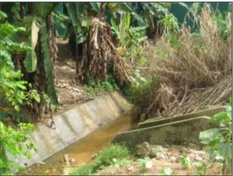
Location 3: This location is the most downstream point of the channel on Farm 85 Trading property, immediately upstream of the sand storage area. This location is depicted in Figure 6.

(23)

23

Figure 3: Map of land use and sampling locations in Neo Tiew subcatchment.

(24)

24

Figure 4: Sampling location 1.

(25)

25

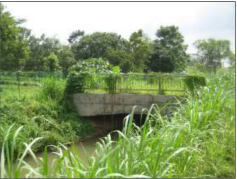
Location 4: This sampling location is located on the upstream side of the Neo Tiew Road bridge over the drainage channel. This location is the closest accessible point to the downstream edge of the sand storage property. The sampling location can be seen in Figure 7.

Location 5: Samples were collected immediately downstream of the Neo Tiew Road bridge. Though physically proximate to Location 4, an outfall draining the adjacent sugar cane fields enters the drainage channel between the two sampling points. This sampling location is presented in Figure 8.

Location 6: This location is the downstream side of the pedestrian bridge adjacent to Bollywood Farm. This location was selected in an effort to assess the nutrient and bacteria contributions from Bollywood Farm. The location is depicted in Figure 9.

Location 7: Location 7 was used as a placeholder for field blanks. Blank sample collection methods are described in the following section.

Location 8: Samples were collected from a parallel drainage channel on Farm 85 Trading property. The location was approximately midway between sampling locations 2 and 3 and solely includes drainage from Farm 85 Trading. An image of the sampling location can be seen in Figure 10.

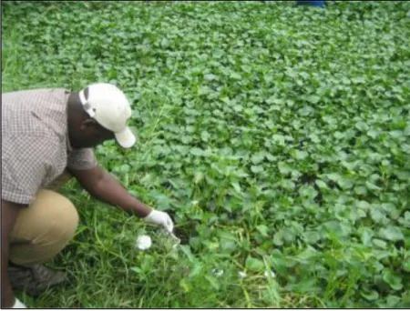
Location 9: Samples were collected from the rainwater collection pond at Green Circle Farm, which is an organic fruit and vegetable farm. Farm personnel indicated that the pond is approximately 6 m deep, but samples were only taken near the water surface. There is a thick layer of vegetation on the top of the pond, as can be seen in Figure 11.

Geographic coordinates of each sampling location and additional location information can be found in Appendix A.

(26)

26

(27)

27

(28)

28

3.1.2 Weather conditions

Samples were collected under both dry and wet weather conditions in order to provide as complete an understanding of catchment runoff water quality as possible. Rainfall was measured with a RIMCO 8020 tipping bucket rain gauge (McVan Instruments Pty. Ltd, Scoresby, Victoria, Australia) with 0.2 mm tip. The rain gauge was installed for the monitoring and sampling of stormwater from the Kranji Catchment under a joint project between Nanyang Technological University and PUB (Le 2013).

On the first day of sampling, January 16, 2013, there was no rain throughout the morning, during which all samples were collected. The most recent rainfall event recorded at the nearby Verde rain gauge station prior to January 16 sampling ended approximately 18 hours before sampling began and totaled 11.8 mm over its duration of approximately one hour (Le 2013).

There was light rain during sampling on January 22, 2013. The rain event began 3 hours before the start of sampling and ceased shortly after sampling began. Total precipitation from the event, as measured at the Verde station, was 1.2 mm (Le 2013).

3.1.3 Sample collection

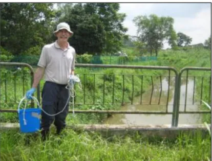
All water samples were manually collected as grab samples during January field collection. Water was collected from the drainage channel either directly in laboratory glassware and Nasco Whirl-Pak® (Nasco, Fort Atkinson, WI) collection bags or, in sampling locations in which direct manual physical to the channel was not feasible due to topography or vegetation, using a 10-liter bucket and rope. Equipment used for collection by bucket can be seen in Figure 12. The bucket was rinsed with water from each sample location prior to collecting the sample volume. Immediately following collection by the bucket method, water samples were transferred to laboratory glassware and Whirl-Pak® bags. Samples taken at each location consisted of one liter collected in a brown glass laboratory bottle, two 530-mL Whirl-Pak® bags, and one brown glass 40-mL vial. The large glass bottles were prepared by Setsco Services Pte. for sample collection

(29)

29

and thus were not rinsed or otherwise altered prior to on-site sample collection. Sterile Whirl-Pak® bags were unsealed immediately prior to sample collection in each location. The 40-mL glass vials were rinsed thoroughly with sample water prior to being filled.

Figure 12: Bucket collection equipment at sampling location 6.

Upon sample collection, the 1-L bottles and Whirl-Pak® bags were stored on ice for field preservation and subsequently transferred to a 4oC refrigerator until laboratory analysis was completed. All holding time practices were conducted in accordance with EPA standards (EPA 1979). The 40-mL glass vial sample from each location was collected for ammonia nitrogen (NH-N) analysis and thus was preserved accordingly until time of analysis. For adequate preservation, 0.05 mL of concentrated sulfuric acid (H2SO4) was added in the field to each

40-mL sample in accordance with EPA standard method 350.1 (EPA 1979). Following the addition of sulfuric acid, samples were stored on ice until analysis was completed.

A field blank was prepared and transported on each day of sampling in order to provide insight into the reliability of the sample collection and analysis process. The blank consisted of deionized water collected directly into Whir-Pak® bags and laboratory glassware immediately prior to field collection of samples. The blank samples were transported on ice during sample collection and refrigerated identically to field samples. Analysis of the blank sample was performed in accordance with the same standards and procedures as those applied to field samples.

3.1.4 Flow determination

In order to estimate flow volume and thus pollutant loads, channel dimensions were measured at locations of supercritical flow under both dry and wet conditions. Sampling locations 2 and 8 were such areas of supercritical flow, both of which can be approximately represented as geometric channels with critical flow for the purpose of flow determination. Channel dimensions and depth of flow were then used in conjunction with the appropriate hydraulic equations to determine flow rates at these sampling locations.

(30)

30

Wet conditions were observed on the morning of January 22, 2013 after 3 hours of precipitation totaling 1.2 mm. Dry conditions were observed on the morning of January 25, 2013, with the most recent precipitation event having ceased 17 hours prior to observation (Le 2013).

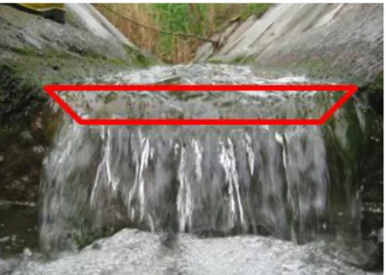
The supercritical flow region at sampling location 2 can be approximated by a trapezoidal channel, as seen in Figure 13. The respective flow region at sampling location 8 can be represented by a circular channel, as seen in Figure 14.

Figure 13: Supercritical flow region at sampling location 2 with overlaid trapezoid.

Figure 14: Supercritical flow region at sampling location 8 with overlaid arc.

The depth of flow at each of these locations of supercritical flow is approximately equivalent to critical depth, which, along with other relevant dimensions, can be related to channel flow by Equations 1 and 2 (Brater and King 1976):

(31)

31 For flow in trapezoidal channels:

√ (1)

For flow in circular channels:

(2)

In which:

 Q = channel flow (m3

/s)

 g = acceleration due to gravity (m/s2

)

 b = width of bottom of trapezoidal channel (m)

 z = slope of sides of trapezoidal channel (dimensionless)  Dc = critical depth (m)

 θ = angle from center of channel to edge of flow (radians)

Using the above-listed equations and dimensions collected in the field, the following flow rates were calculated (Table 2). Measured channel dimensions are provided in Appendix B.

Table 2: Calculated channel flow at locations 2 and 8.

Date Flow, location 2

(trapezoidal)

Flow, location 8 (circular)

1/22/2013 (wet weather) 350 m3/day 69 m3/day 1/25/2013 (dry weather) 150 m3/day 26 m3/day

3.1.5 Chemical and biological analysis

The collected samples were analyzed for total nitrogen (TN), ammonia nitrogen (NH-N), nitrate nitrogen and nitrite nitrogen (NO-N), total phosphates (TP), total dissolved phosphorus (TDP), total organic phosphorus (TOP), total suspended solids (TSS), total coliform, E. coli, and enterococci. Bacterial analyses (total coliform, E. coli, and enterococci) were performed using IDEXX Quanti-Trays and growth media (IDEXX Laboratories, Inc., Westbrook, ME, USA). Analyses of NH-nitrogen, NO-nitrogen, and TP were performed using CHEMetrics Vacu-vials® and photometric analysis (CHEMetrics, Inc., Midland, VA, USA). TSS, TN, TOP, and TDP for all sampling locations, as well as NO-N nitrate nitrogen for selected locations, were analyzed by an external laboratory, Setsco Services Pte., according to American Public Health Association (APHA) standard procedures (APHA 2012).

Analyses of NO-nitrogen (both nitrite and nitrate species), NH-nitrogen, and total phosphate were performed on the same day as sampling. Samples taken for bacterial analysis were stored in a refrigerator at a temperature of 4oC for approximately 24 hours prior to serial dilution and incubation. The water samples collected in 1-L glass bottles were delivered to Setsco Services Pte. on the same day of sampling for analysis of total suspended solids, total organic phosphorus, total dissolved phosphorus, and total nitrogen.

(32)

32

3.1.5.1.1 CHEMetrics chemical analysis

Analysis of nitrate and nitrite nitrogen, ammonia nitrogen, and total phosphates were performed using CHEMetrics Vacu-vials® and colorimetric analysis. The analytical kits for each chemical species were used in accordance with the manufacturer’s instructions, which comply with applicable APHA and EPA analytical procedures (CHEMetrics 2012).

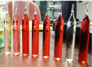
Nitrate-N concentration was determined using a reduction of nitrate to nitrite in the presence of zinc and other chemicals provided in the CHEMetrics analysis kit, ultimately resulting in a pink-hued solution, the color of which is proportional to the concentration of nitrate present (CHEMetrics 2012b). Vials of prepared nitrate-N solution can be seen below in Figure 15. A photometer set to the appropriate CHEMetrics analytical program was used to translate the resultant color to the nitrate-N concentration. Samples were prepared and analyzed in accordance with CHEMetrics procedure K-6913, which meets APHA standard 4500-NO3- E and EPA

method 353.3 (CHEMetrics 2012b). Samples collected at locations 1, 3, 4, 5, 6, and 8 were over the nitrate-N concentration range quantifiable by the CHEMetrics method, so nitrate-N analysis on these samples was performed by the external analytical laboratory.

Figure 15: Nitrate samples prepared for colorimetric analysis using CHEMetrics method.

The CHEMetrics method of nitrite-N analysis relies on the formation of an azo dye from nitrite in an acidic solution in the presence of organic substances. The manufacturer’s procedure, K-7003, is compliant with APHA method 4500-NO2- B and EPA method 354.1 (CHEMetrics

2012c).

CHEMetrics analysis of ammonia-N follows the salicylate method, in which monochloramine reacts with salicylate to produce 5-aminosalicylate, the green color of which is used for photometric ammonia concentration determination. Ammonia sample preparation and analysis was performed in accordance with CHEMetrics procedure K-1403, compliant with EPA method 350.1 (CHEMetrics 2012d).

Total phosphate analysis is performed by an acid digestion process in which phosphates are converted to orthophosphate. Reaction of orthophosphates with chemicals in the CHEMetrics solution results in a blue complex to enable colorimetric analysis. Analysis was performed

(33)

33

following the manufacturer’s procedure K-8540, which meets APHA standards 4500-P B.5 and E, as well as EPA methods 365.2 and 365.4 (CHEMetrics 2012e). All analyses were performed on the same day of sampling and analyzed using a CHEMetrics Model V-2000 photometer.

3.1.5.2 Bacterial analysis

Determination of bacterial contaminant concentration in samples was performed using IDEXX Quanti-Tray®/2000 in conjunction with IDEXX Enterolert and Colilert growth substrates (IDEXX Laboratories, Inc., Westbrook, Maine). In this method, a 100-mL volume of water sample is combined with the appropriate substrate and deposited in a calibrated, sterilized tray and subsequently incubated to enable appropriate bacterial growth. The results of this process are used to determine the Most Probable Number of colony-forming bacteria per 100 mL (MPN/100 mL) (IDEXX 2012). Separate samples must be prepared for analysis of enterococci using Enterolert and E. coli using Colilert. Sample trays prepared using Colilert serve a dual purpose, resulting in counts of both total coliform and E. coli (IDEXX 2012).

Quanti-Tray/2000 methods facilitate determination of bacterial concentrations ranging from 0 to 2,419.6 MPN/100 mL (IDEXX 2012). Since agricultural samples from the Neo Tiew subcatchment had been previously demonstrated to sustain bacterial concentrations greater than this quantifiable range (Bossis 2011, Dixon et al. 2009), serial dilutions were used to increase the quantifiable range of the analytical method. In the first set of collected samples, water samples from locations 1 and 2 were diluted and prepared at ratios of 1, 1:100, and 1:10,000. Samples collected from all other sampling locations, and all samples from the second day of field collection, were diluted and prepared at ratios of 1:10, 1:1,000, and 1:100,000 due to high anticipated bacterial concentrations. All dilutions were prepared with sterilized glassware and deionized water in order to minimize potential sources of laboratory contamination.

Enterolert and Colilert growth substrates were then added to each dilution, resulting in six total samples from each sampling location. Each sample and substrate mixture was then deposited in a Quanti-Tray/2000, sealed, and incubated for 24 to 28 hours. Enterococci samples were incubated at 41oC, and total coliform/E. coli samples were incubated at 35oC, in accordance with manufacturer specifications (IDEXX 2012).

After adequate incubation, concentration of the respective types of bacteria is determined by counting the number of positive and negative wells in each Quanti-Tray/2000. In the trays using Colilert substrate, wells that are positive for total coliform are yellow in color, as can be seen in Figure 16. Under a 6-watt, 365-nm ultraviolet light, wells on the same tray that are positive for E. coli fluoresce to a yellow shade. When trays using Enterolert growth media are viewed under ultraviolet light, wells positive for Enterococci fluoresce to a blue shade (IDEXX 2012), as can be seen in Figure 17.

(34)

34

Figure 16: Total coliform presence in Quanti-Tray/2000. Yellow wells are positive for total coliform.

Figure 17: Enterococci presence in Quanti-Tray/2000. Blue fluorescent wells are positive for enterococci. Counts of positive and negative wells in each tray are used with the IDEXX Most Probable Number table to determine the MPN for each bacterial type at each dilution. Given that each water sample has three dilutions, there are three possible concentrations to use as the appropriate MPN for each sample, at least one of which is within the range of the upper and lower detection limits. In addition to the MPN for a given positive well count, IDEXX provides a statistical range for each positive count. Thus, the selected value of MPN for each sample is the dilution for which the statistical range is smallest. MPN and statistical range values were multiplied by the appropriate dilution factor to account for the adjusted concentrations.

(35)

35

3.1.5.3 External laboratory

Certain chemical analyses were outside the scope of the limited laboratory resources available during the field work period, and thus were performed by a third-party analytical laboratory, Setsco Services Pte., Singapore. Samples to be analyzed by Setsco were collected in glassware provided by the laboratory, preserved on ice during field collection, and delivered to the laboratory within four hours of sample collection.

Setsco performed analyses of total suspended solids, total nitrogen, total organic phosphates, and total dissolved phosphates for all sampling locations, as well as nitrate nitrogen on samples from the locations that were outside the CHEMetrics quantifiable range.

External laboratory analyses were performed in accordance with the following APHA standard procedures (APHA 2012): TSS – APHA: Pt 2540D; TN – APHA: Pt 4500-N org; OP – APHA: Pt 4500-P (G); TDP – APHA: Pt 4500-P (H), and nitrate – APHA: Pt 4500-NO3 (I).

3.2 Results

The full set of measured concentrations can be seen in Appendix C.

3.2.1 Nutrients

A broad range of nutrient concentrations were observed in sampling locations along the main drainage channel. The minimum and maximum values observed for each nutrient contaminant on each sampling day can be seen in Table 3.

Table 3: Range of observed nutrient concentrations.

1/16/13 1/22/13 Nutrient Min (mg/L) Max (mg/L) Min (mg/L) Max (mg/L) Total N 1.8 19.8 4.03 18.1 Nitrate-N 0.3 16.8 1.07 17.0 Nitrite-N 0.08 0.23 0.09 0.24 Ammonia-N 0.04 2.14 0.52 2.66 TP 0.52 2.12 0.27 1.6 TDP 0.16 1.27 0.12 1.2 TOP 0.034 1.04 0.006 0.22

It is clear from the results in Table 3 that nutrient concentrations were not steady throughout the reach of the drainage channel but rather varied by location, so it is important to understand where the maxima and minima occurred. The observed nutrient concentrations at each sampling location, plotted from the most upstream sampling location to the most downstream sampling location, are presented in Figures 18, 19, 20, and 21. As can be seen in Figures 18 and 19, the maximum observed values of total nitrogen and nitrate nitrogen occurred at location 3 on both sampling days. The magnitude of the maximum observed concentrations of TN and NO3-N were

similar across the two sampling days as well, with TN values of 19.8 and 18.1 mg/L on 1/16/13 and 1/22/13, respectively, and NO3-N values of 16.8 and 17 mg/L on 1/16/13 and 1/22/13,

(36)

36

sampling location 3. There was greater variation in maximum phosphorus species concentrations across the two days of sampling, particularly in total organic phosphorus, with a value of 1.04 mg/L on 1/16/13 and 0.22 mg/L on 1/22/13. Though sampling location 3 presented maximum concentrations for most of the nutrient constituents, peak ammonia nitrogen was observed at sampling location 2 on both sampling days. The maximum observed NH-N values were similar across both days of sampling, with values of 2.14 and 2.66 mg/L on 1/16/13 and 1/22/13, respectively.

Though there is some variation across nutrient species and sampling days, a general trend is evident in Figures 18, 19, 20, and 21. There is no strong trend between sampling locations 1 and 2, with some contaminants decreasing, others increasing, and still others holding steady. However, with the exception of ammonia nitrogen and nitrite nitrogen, a clear trend emerges at location 3. At location 3, most nutrient species significantly increase, and then subsequently decrease at location 4, remaining fairly steady through locations 5 and 6. Ammonia nitrogen exhibits a similar trend, except with the strong peak at location 2. Nitrite nitrogen does not exhibit any strong peak, but rather maintains a fairly constant and low magnitude across all sampling locations.

(37)

37

Figure 19: Nitrogen concentrations on 1/22/13.

(38)

38

Figure 21: Phosphorus concentrations on 1/22/13.

In addition to the samples collected along the reach of the main drainage channel, the additional locations sampled present interesting trends in nutrient concentration. These additional sampling locations, referred to previously as locations 8 and 9, have been inserted into the graphs of nutrient concentrations along the reach of the drainage channel in order to elucidate the approximate contribution of each of the drainage areas that they represent, as can be seen in Figures 22, 23, 24, and 25. Location 8, the parallel drainage channel on the Farm 85 Trading plot, has been inserted between locations 2 and 3 to represent the contributions from the activities at Farm 85 Trading, and location 9, the pond at Green Circle Farm, has been inserted between locations 1 and 2, though Green Circle Farm is not the sole contributor to runoff between locations 1 and 2.

As can be seen in Figures 22 and 23, the parallel drainage channel at Farm 85 Trading presents much higher concentrations of total nitrogen and nitrate nitrogen than in the main drainage channel at location 3, with values of 81.3 mg/L total nitrogen and 78.8 mg/L nitrate nitrogen on 1/16/13 and 55 mg/L total nitrogen and 53.2 mg/L nitrate nitrogen on 1/22/13. Though the flow in the parallel channel is less than that of the main channel and thus a comparison of the concentrations at locations 8 and 3 is not a direct one, the high total nitrogen and nitrate nitrogen concentrations in the parallel channel may help to explain the high concentrations observed at location 3.

Similarly, the highest observed ammonia nitrogen value was in the pond at Green Circle Farm (location 9) on 1/22/13, with a value of 2.77 mg/L. This overall maximum value immediately precedes the maximum value observed in the main channel at location 2 and can help to explain the trend observed for ammonia in the main drainage channel. The maximum value of total dissolved phosphorus concentration was also observed in the Green Circle pond, 2.07 mg/L,

(39)

39

which was nearly twice the highest observed in any location in the main drainage channel. There was also a spike in total phosphate concentration in the Green Circle pond, though it did not exceed the maximum value observed on that day of sampling, which occurred at location 3.

Figure 22: Nitrogen concentrations with additional points, 1/16/13.

(40)

40

Figure 24: Phosphorus concentrations with additional points, 1/16/13.

Figure 25: Phosphorus concentrations with additional points, 1/22/13.

3.2.2 Bacteria

Bacterial counts were observed to vary not only by location along the sampling channel, but also by date of sampling. There were also large differences in concentration between the different types of bacteria. A summary of the minimum and maximum concentrations observed on each day of sampling for each type of bacteria can be seen in Table 4.

(41)

41

Table 4: Range of measured bacteria concentrations.

1/16/13 1/22/13

Bacteria type Min

(MPN/100 mL) Max (MPN/100 mL) Min (MPN/100 mL) Max (MPN/100 mL) Total coliform 155,000 1,050,000 125,000 687,000 E. coli 934 45,700 1,330 166,000 Enterococci 1,790 11,600 3,650 50,400

As can be seen from the results presented in Table 4, the measured total coliform concentrations were orders of magnitude greater than those measured of either E. coli or enterococci. Among all types of bacteria, concentrations varied significantly along the reach of the main drainage channel. Comparisons of bacterial concentration at each sampling location on each sampling date, plotted from the most upstream to the most downstream location, can be seen in Figures 26 and 27. On both days sampled, the peak value of total coliform occurred at sampling location 3, the most downstream location on Farm 85 Trading property. The maximum concentrations of E. coli and enterococci occurred at location 2 on both sampling days. In general, the bacterial concentration trend along the reach of the drainage channel is similar to that of nutrient concentrations. Maximum concentrations for all observed bacterial constituents and on both sampling days occur at either location 2 or 3, with concentrations decreasing at location 4 and remaining relatively steady throughout the remainder of the channel.

Though the locations of the maxima for each bacterial constituent were temporally consistent, the magnitudes of the maximum concentrations measured on the two days of sampling were different. Under dry conditions on 1/16/13, maximum total coliform concentration was greater than 1,000,000 MPN/100 mL, while under wet conditions on 1/22/13, the maximum value was considerably lower at 687,000 MPN/100 mL. The maximum concentrations for E. coli and enterococci also changed between the two sampling days, but the direction of the change was opposite to that for total coliform, with greater concentrations under wet conditions than under dry, as can be seen in Table 4.

The samples collected at points outside the main drainage channel also provide information about bacterial sources in the Neo Tiew drainage area. As with the nutrient results, these additional sampling locations, referred to previously as locations 8 and 9, have been inserted into the graphs of bacterial counts along the reach of the drainage channel in order to elucidate the approximate contribution of each of the drainage areas that they represent, as can be seen in Figures 28 and 29.

(42)

42

Figure 26: Bacterial counts on 1/16/13.

(43)

43

For all analyzed bacterial constituents, the observed concentrations in the parallel drainage channel at Farm 85 Trading were lower than those observed at the surrounding points, locations 2 and 3. Conversely, the sample taken from the pond at Green Circle Farm on 1/22/13 contained the highest observed concentrations of total coliform and enterococci, with values of 3,090,000 MPN/100 mL total coliform and 142,000 MPN/100 mL enterococci. When compared to the maximum concentrations observed within the main drainage channel, which were 1,050,000 MPN/100 mL total coliform (at location 3 on 1/16/13) and 50,400 MPN/100 mL enterococci (at location 2 on 1/22/13), it is evident that the pond at Green Circle is a particularly concentrated source of bacteria. The observed concentration of E. coli in the Green Circle pond was less than the value observed at location 2 on the same day of sampling.

Figure 28: Bacterial counts with additional points, 1/16/13.

(44)

44

3.2.3 Solids

The concentration of total suspended solids in each water sample taken was also analyzed. The TSS concentration at each sampling location can be seen in Figures 30and 31. Trends along the reach of the main drainage channel were consistent across both sampling days, with a strong peak solids concentration at location 3 and relatively similar and low TSS concentrations at all other sampling locations. The maximum TSS observed on 1/16/13 was 37.2 mg/L and the maximum observed on 1/22/13 was 28.4 mg/L TSS. Though more suspended solids might be anticipated under the wet conditions on 1/22/13, the maximum observed TSS concentration was greater under the dry conditions on 1/16/13.

Figure 30: Total suspended solids, 1/16/13.

(45)

45

3.2.4 Field blanks and duplicates

In order to understand the reliability and repeatability of the field sampling program and the laboratory analyses procedures, field blanks were collected and analyzed and one sample was analyzed in duplicate.

Results of field blank analysis can be seen in Table 5. Concentrations for nearly all analyses on both sampling days were either below the relevant detection limit or very near the detection limit. The one notable exception, however, is the total phosphates result in the blank from 1/16/13, in which the result, 0.81 mg/L, was not only much greater than the detection limit of 0 mg/L (CHEMetrics 2012e), but it was also among the highest total phosphate concentrations observed on that day of sampling. This troubling result was not repeated in the second set of samples and analyses, however, which indicates that it was more likely the result of sample contamination or insufficiently cleaned glassware rather than a flawed sampling or analysis procedure.

Table 5: Field blank analysis results, 1/16/13 and 1/22/13.

Analyte 1/16/13 1/22/13 Total nitrogen (mg/L) <0.01 <0.01 Nitrate-N (mg/L) 0.08 0.03 Nitrite-N (mg/L) 0.01 0.01 Ammonia-N (mg/L) 0.03 <0.01 Total phosphates (mg/L) 0.81 0.08 Total dissolved P (mg/L) 0.0081 0.015 Total organic P (mg/L) 0.09 0.099

Total suspended solids (mg/L) <2 <2 Total coliform (MPN/100 mL) <1 <1

E. coli (MPN/100 mL) <1 <1

Enterococci (MPN/100 mL) <1 <1

Duplicate analytical tests were performed on the sample collected at location 2 on 1/22/13 for all analyses that were performed in-house. The duplicate results can be seen in Table 6. For most nutrient analyses, the measured concentrations in the original sample and the duplicate sample were similar, with the exception of the ammonia-N result. There was a 220% discrepancy between the ammonia-N concentrations of the duplicate samples, which may be attributable to inadequate mixing of the sample prior to decanting into analytical glassware. The second sample analyzed, 2-2D, contained the volume from the bottom of the collection glassware, which would contain any settled material and thus potentially account for the significantly higher concentration of ammonia-N. The bacterial counts in the sample and the duplicate were relatively similar, with the largest variation being 15% in the E. coli count. In general, the results of the duplicate analyses demonstrate repeatability in the laboratory analytical procedures.