Context-dependent modeling in a segment-based speech recognition system

(1)

Context-Dependent Modeling in a Segment-Based

Speech Recognition System

by

Benjamin M. Serridge

B.S., MIT, 1995

Submitted to the Department of Electrical Engineering

and Computer Science

in partial fulfillment of the requirements for the degree of

Master of Engineering in Electrical Engineering and Computer Science

at the

MASSACHUSETTS INSTITUTE OF TECHNOLOGY

Augist 1997

@ Benjamin M. Serridge, MCMXCVII. All rights reserved.

The author hereby grants to MIT permission to reproduce and

distribute publicly paper and electronic copies of this thesis document

in whole or in part, and to grant others the right to do so.

Author ... ...

.. ...

.... ...

Department of Electrical Engineering

and Computer Science

August 22, 1997

Certified by...

...

7

Dr. James R. Glass

Principal Research Scientist

.

-T-a w

Supervisor

Accepted by ... .

_..

Arthur C. Smith

Chairman, Departmental Committee on Graduate Theses

(2)

Context-Dependent Modeling in a Segment-Based Speech Recognition System

by

Benjamin M. Serridge

Submitted to the Department of Electrical Engineering and Computer Science

on August 22, 1997 in partial fulfillment of the requirements for the degree of

Master of Engineering in Electrical Engineering and Computer Science

Abstract

The goal of this thesis is to explore various strategies for incorporating contextual information into a segment-based speech recognition system, while maintaining com-putational costs at a level acceptable for implementation in a real-time system. The latter is achieved by using independent models in the search, while dependent models are reserved for re-scoring the hypotheses proposed by the context-independent system.

Within this framework, several types of context-dependent sub-word units were evaluated, including word-dependent, biphone, and triphone units. In each case, deleted interpolation was used to compensate for the lack of training data for the mod-els. Other types of context-dependent modeling, such as context-dependent boundary modeling and "offset" modeling, were also used successfully in the re-scoring pass.

The evaluation of the system was performed using the Resource Management task. Context-dependent segment models were able to reduce the error rate of the context-independent system by more than twenty percent, and context-dependent boundary models were able to reduce the word error rate by more than a third. A straight-forward combination of context-dependent segment models and boundary models leads to further reductions in error rate.

So that it can be incorporated easily into existing and future systems, the code for re-sorting N-best lists has been implemented as an object in Sapphire, a frame-work for specifying the configuration of a speech recognition system using a scripting language. It is currently being tested on Jupiter, a real-time telephone based weather information system under development here at SLS.

(3)

Acknowledgments

My experiences in the Spoken Language Systems group have been among the most valuable of my MIT education, and the respect I feel for my friends and mentors here has only grown with time. Perhaps more important than the help people have given me in response to particular problems is the example they set for me by the way they guide their lives. I would especially like to mention my advisor Jim, who has demonstrated unwavering support for me throughout the past year, and my office mates Sri and Giovanni, who have made room NE43-604 something more than an office over the past year. It is because of the people here that, mixed with my excitement about the future, I feel a tinge of sorrow at leaving this place.

(4)

List of Figures

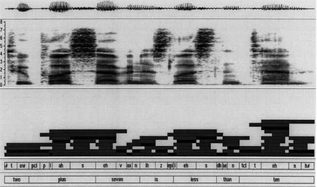
1-1 A spectrogram of the utterance "Two plus seven is less than ten." Notice the variation in the realizations of the three examples of the phoneme /eh/: the first, in the word "seven," exhibits formants (shown in the spectrogram as dark horizontal bands) that drop near the end of the phoneme as a result of the labial fricative /v/ that follows it; the second /eh/, in the word "less," has a second formant that is being "pulled down" by the /1/ on the left; and the third /eh/, in the word "ten," has first and third formants that are hardly visible due to energy lost in nasal cavities that have opened up in anticipation of the final /n/. If such variations can be predicted from context (as is believed to be the case), then speech recognition systems that do so will embody a much more precise model of what is actually occuring during natural

speech than those that do not ... 12 2-1 Part of a pronunciation network spanning the word sequence "of the." 19 2-2 A sample Viterbi lattice, illustrating several concepts. An edge

con-nects lattice nodes (1,1) and (2,3) because 1) there is an arc in the pronunciation network between the first and the second node, and 2) there is a segment between the first and the third boundaries. The edge is labeled with the phonetic unit /ah/, and its score is the score of the measurement vector for segment 82 according to the acoustic

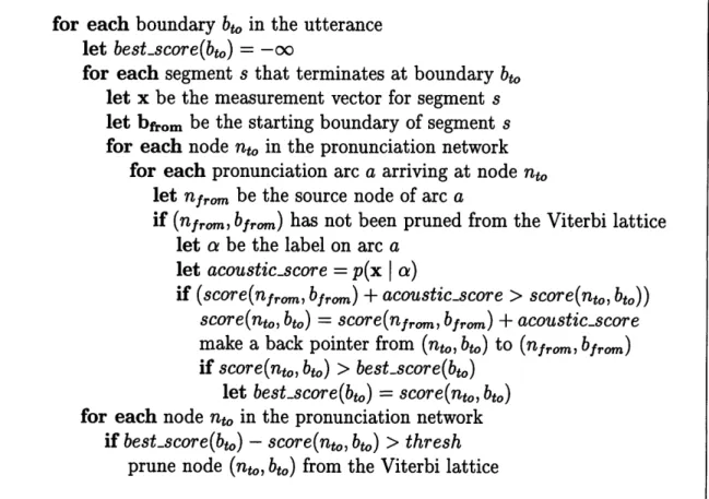
model for /ah/. (Note that not all possible edges are shown.) Of the two paths that end at node (5, 5), only the one with the higher score will be maintained. ... ... . 20 2-3 A more concise description of the (simplified) Viterbi algorithm. . . . 22 2-4 A re-sorted N-best list. The first value is the score given by the

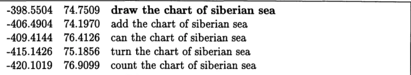
resort-ing procedure, while the second is the original score from the A* search. Notice that the correct hypothesis (in bold) was originally fourth in the N-best list according to its score from the A* search. ... . 25 3-1 A plot of word and sentence error rate for an N-best list as a function

of N. The upper curve is sentence error rate. . ... 32 B-1 The algorithm for computing the limiting state probabilities of a Markov

(8)

C-1 A histogram of the results of 50 different sets of models evaluated on

test89, as described in Table C-1. Overlayed is a Gaussian distribution with the sample mean and sample variance as its parameters... 70

(9)

List of Tables

3-1 The best results in the literature published for Resource Management's Feb. 1989 evaluation. (The error rates of 3.8% are actually for a slightly different, but harder test set.) ... ... 29 3-2 Baseline results for context-independent models on test89. ... . 30 3-3 Word and sentence error rate on test89 as the length of the N-best list

increases. ... 33

5-1 The number of contexts represented in the training data for each type of context-dependent model, with cut-offs of either 25 or 50 training tokens . . . . . . . ... 39 5-2 Test-Set Coverage of context-dependent models. . ... 40 5-3 Summary of the performance of several different types of

context-dependent models. ... 40

5-4 Summary of the performance of several different types of context-dependent models. For comparison purposes, the first two columns are the results from Table 5-3, and the last two columns are the results of the same models, after being interpolated with context-independent models. The numbers in parentheses are the percent reduction in word error rate as a result of interpolation. . ... 41 5-5 Results of experiments in which triphone models were interpolated

with left and right biphone models and context-independent models, in various combinations. In no case did the word error rate improve over the simple interpolation with the context-independent models only. 42 5-6 Percent reduction in word error rate, adjusted to account for

test-set coverage. The model test-sets are all interpolated with the context-independent models. (The last two rows refer to triphone-in-word models, not previously discussed.) ... . ... 43 5-7 The results of various combinations of backoff strategies. The

perfor-mance is essentially the same for all combinations, and does not repre-sent an improvement over the increased coverage that can be obtained by decreasing the required number of tokens per model. ... 44 5-8 A comparison of the performance of word-dependent models in the

Viterbi search and in the re-sorting pass. Performance is slightly better in the Viterbi search, though the differences are not very statistically significant (each result is significant to within 0.25%). ... . 45

(10)

6-1 Summary of results from boundary model experiments. The numbers in parentheses are the percent reduction in word error rate achieved by the re-scoring over the results of the context-independent system. For comparison purposes, results are also presented for the 25+ version of the catch-all models, defined similarly to the 50+ models described above, except that only 25 examples are required to make a separate m odel . . . . 50 6-2 Word error rates resulting from the possible combinations of boundary

models with word-dependent models. . ... 51 7-1 Summary of the performance of several variations of the offset model

strategy. ... 55

7-2 The performance of triphone models, both in the normal case and as a combination of left and right biphone models. . ... 55 7-3 Performance of right biphone models when tested on data adjusted

ac-cording to offset vectors. The first row is the normal case, where offsets between triphone contexts and context-independent units are used to train adjusted context-independent models, which are applied in the re-sorting pass as usual. The second row uses the same offset vectors, but instead trains right-biphone models from the adjusted training data, applying these right biphones in the resorting pass. Finally, the third row trains offset vectors between triphone and right biphone contexts, applies these offsets to the training data, from which are trained right biphone models. These offsets and their corresponding right biphone models are applied in the resorting pass as per the usual procedure. 56 A-1 Definition of the 40 measurements taken for each segment in the

ex-periments described in this thesis. . ... . 60 B-1 A comparison of three interpretations of the word pair grammar. . . . 65

C-1 Statistics of the variation encountered when 50 model sets, each trained

under the same conditions on the same data, are tested on two different

(11)

Chapter 1 Context-Dependent Modeling

1.1 Introduction

Modern speech recognition systems typically classify speech into sub-word units that loosely correspond to phonemes. These phonetic units are, at least in theory, inde-pendent of task and vocabulary, and because they constitute a small set, each one can be well-trained with a reasonable amount of data. In practice, however, the acoustic realization of a phoneme varies greatly depending on its context, and speech recogni-tion systems can benefit by choosing units that more explicitly model such contextual effects.

The goal of this thesis is to comparatively evaluate some strategies for modeling the effects of phonetic context, using a segment-based speech recognition system as a basis. The next section provides, by way of an overview of previous research on the topic, an introduction to several of the issues involved, followed by an outline of the remaining chapters of this thesis and a more precise statement of its objectives.

1.2 Previous Research

Kai-Fu Lee, in his description of the SPHINX system [17], presents a clear summary of the search for a good unit of speech, including a discussion of most of the units considered in this thesis. He frames the choice of speech unit in terms of a tradeoff between trainability and specificity: more specific acoustic models will, all else being equal, perform better than more general models, but because of their specificity they are likely to occur very rarely and are therefore difficult to train well. Very general models, on the other hand, can be well-trained, but are less likely to provide a good match to any particular token.

Since the goal of speech recognition is to recognize the words a person speaks, the most obvious choice of speech unit is the word itself. In fact, word models have been applied fairly successfully in small-vocabulary systems to problems such as the connected-digit recognition task [24]. Unfortunately, word models do not generalize well to larger vocabulary tasks, since the data used to train one word can not be shared by others. A more linguistically appealing unit of speech is the phoneme,

(12)

Figure 1-1: A spectrogram of the utterance "Two plus seven is less than ten." Notice the variation in the realizations of the three examples of the phoneme /eh/: the first, in the word "seven," exhibits formants (shown in the spectrogram as dark horizontal bands) that drop near the end of the phoneme as a result of the labial fricative /v/ that follows it; the second /eh/, in the word "less," has a second formant that is being

"pulled down" by the /1/ on the left; and the third /eh/, in the word "ten," has first and third formants that are hardly visible due to energy lost in nasal cavities that have opened up in anticipation of the final /n/. If such variations can be predicted from context (as is believed to be the case), then speech recognition systems that do so will embody a much more precise model of what is actually occuring during natural speech than those that do not.

(13)

since a small set of units covers all possible utterances. This generality allows data to be shared across words, but at the same time forces each acoustic model to account for all the different possible realizations of a phoneme. Acoustic models can handle the variability within a phoneme implicitly if they are constructed as mixtures of several simpler component models. Previous research, however, has shown that superior performance can be obtained by handling the variation explicitly. Gender or speaker-dependent models, for example, create a separate model for each gender or speaker. Similarly, context-dependent models create a separate model for each context.

Many types of context-dependent models have been proposed in the literature. "Word-dependent" phone models, first proposed by Chow et al in 1986 [3], consider the context of a phone to be the word in which it occurs. Kai-Fu Lee applied such models in the SPHINX system to a small set of 42 "function words", such as of, the, and with, which accounted for almost 50% of the errors in the SPHINX system on the Resource Management task [17]. Adding these models to the context-independent system reduced the error rate by more than 25%, significantly decreasing the number of errors in both function words and non-function words.

More commonly used are phone models that are conditioned on the identity of the neighboring phones. A left biphone is dependent on the preceding phone, while a right biphone is dependent on the following phone. A triphone model depends on both the left and the right context. Such models were first proposed by Bahl et al in 1980 [1], and since then have been shown many times to improve the performance of various systems [26, 18]. The concept has even been extended to the use of quinphones which take into account the identity of the two following and preceding phones [29].

The aforementioned models all adhere to the same basic paradigm: the data that normally would contribute to the construction of just one model are grouped according to context, thus creating a separate model for each context. Unfortunately, if the number of possible contexts is large, the amount of data available to each model will be small.

This problem, known as the sparse data problem, can be dealt with in several ways. The simplest technique is to train models only for those units for which sufficient training data are available [16]. A more sophisticated (but not necessarily better) approach is to merge together contexts that have similar effects, thereby not only increasing the amount of training data per model, but also reducing the number of models that must be applied during recognition. The choice of models to be combined can be made either a priori (e.g., using the linguistic knowledge of an expert [19]) or automatically (e.g., using decision trees to split the data according to context [14], unsupervised clustering algorithms to merge the models themselves [17], or other methods).

Even after taking the above precautions, context-dependent models may still per-form poorly on new data, especially if they have been trained from only a few exam-ples. A technique known as "deleted interpolation" aleviates this problem by creating models as a linear combination of context-dependent and context-independent mod-els. The extent to which each component contributes to the final model is calculated from the performance of each model on data that was "deleted" from the training set. This strategy was first applied to hidden Markov models by Jelinek and Mercer

(14)

in 1980 [13] and has been described more recently by Huang et al [11].

Yet another issue raised by the use of context-dependent models is computational complexity, which can grow significantly if, during the search, the recognizer must postulate and test all possible contexts for a given region of speech. The "N-best search paradigm" [2] addresses this issue by using the standard recognizer to produce a list of the top N hypotheses, which are then re-evaluated and re-ranked using more sophisticated modeling techniques.

Most previous research has been performed on systems based on the use of hidden Markov models (HMM's) to perform recognition. The work presented in this thesis is based on SUMMIT [7], a segment-based continuous speech recognition system de-veloped by the Spoken Language Systems group at MIT. Currently, the system used for real-time demonstrations and ongoing research is context-independent, although in the past context-dependent models have been used for evaluation purposes [22, 8]. The Sapphire framework [9] allows speech recognition systems to be constructed as a set of dependencies between individually configured components, and is used as a development platform for the systems described in this thesis. Evaluations are per-formed on the Resource Management task [23], which has been used extensively to evaluate the performance of several fledgling context-dependent systems [18, 15].

1.3 Thesis Objectives

The goal of this thesis is to evaluate different strategies for modeling contextual effects in a segment-based speech recognition system. Included in the evaluation are traditional methods such as word-dependent, biphone, and triphone modeling, as well as some more unusual approaches such as boundary modeling and context normalization techniques (offset models). In all cases, the basic approach is to use context-independent acoustic models to generate a list of hypotheses, which are then re-evaluated and re-ranked using context-dependent models.

The next chapter describes the components of the SUMMIT system relevant to this thesis, including an explanation of the Viterbi search, the A* search, and the algo-rithm used to re-score the hypotheses of the N-best list. Also included is a description of how the re-scoring algorithm is incorporated into the Sapphire framework.

Chapter 3 describes the context-independent baseline system and the Resource Management task. Some preliminary experimental results are presented for the base-line system, as well as some analysis which suggests that the system has the potential to achieve much higher performance, if it can somehow correctly select the best al-ternative from those in the N-best list.

Chapter 4 introduces the technique of deleted interpolation, including a descrip-tion of how it is applied to the models used in this thesis.

Chapter 5 evaluates the performance of word-dependent, biphone, and triphone models, both with and without deleted interpolation. The performance of word-dependent models in the Viterbi is compared with their performance in the resort pass, and results from some experiments with the backoff strategy are given.

(15)

explic-itly modeling the region of speech surrounding the transitions from one phonetic unit to another. Their use in the Viterbi search actually achieves the highest performance documented in this thesis, when combined with the word-dependent models in the resorting pass.

Finally, Chapter 8 summarizes the lessons derived from this thesis and presents some suggestions for future work in this area.

(16)

Chapter 2 The Search

2.1 Introduction

The goal of the search in a segment-based recognizer is to find the most likely word sequence, given the following information:

* the possible segmentations of the utterance and the measurement vector for each segment,

* acoustic phonetic models, which estimate the likelihood of a measurement vec-tor, given the identity of the phonetic unit,

* a language model, which estimates the probability of a sequence of words, and * a pronunciation network, which describes the possible pronunciations of words

in terms of the set of phonetic units being used.

This chapter describes each of these four components separately, and then de-scribes how the search combines them together to produce the final word sequence.

2.2 Components of the Search

2.2.1 Segmentation

The goal of the segmenter is to divide the signal into regions of speech called segments, in order to constrain the space to be searched by the recognizer. From a linguistic point of view, the segments are intended to correspond to phonetic units. From a signal processing point of view, a segment corresponds to a region of speech where the spectral properties of the signal are relatively constant, while the boundaries between segments correspond to regions of spectral change. The segment-based approach to speech recognition is inspired partly by the visual representation of speech presented by the spectrogram, such as the one shown in Figure 1-1, which clearly exhibits sharp divisions between relatively constant regions of speech. Below the spectrogram is a representation of the segmentation network proposed by the segmenter, in which the

(17)

dark segments correspond to those eventually chosen by the recognizer to correspond to the most likely word sequence. The phonetic and word labels at the bottom are those associated with the path represented by the dark segments.

The segmenter used in this thesis operates heuristically, postulating boundaries at regions where the rate of change of the spectral features reaches a local maximum, and building the segment network S from the possible combinations of these boundaries. Since it is very difficult for the recognizer to later recover from a missed segment, the segmenter intentionally over-generates, postulating an average of seven segments for every one that is eventually included in the recognition output [7].

Mathematically, the segment network S is a directed graph, where the nodes in the graph represente the boundaries postulated by the segmenter and an edge connects node ni to node nj if and only if there is a segment starting at boundary bi and ending at boundary bj. The Viterbi search will eventually consider all possible paths through the segment network that start with the first boundary and end with the last.

A measurement vector xi is calculated based on the frame-based observations contained within each segment si [7]. The measurements used in this thesis are a set of 40 proposed by Muzumdar [20]. They consist of averages of MFCC values over parts of the segment, derivatives of MFCC values at the beginning and end of the segment, and the log of the duration of the segment (see Appendix A). From this point onward, the measurement vectors and the segment network are the only information the recognizer has about the signal - gone forever are the frames and their individual MFCC values.

2.2.2 Acoustic Phonetic Models

Acoustic phonetic models are probability density functions over the space of possible measurement vectors, conditioned on the identity of the phonetic unit. A separate acoustic model is created for each phonetic unit, and each is assumed to be inde-pendent of the others. Therefore, the following discussion will refer to one particular model, that for the hypothetical phonetic unit /a/, with the understanding that all others are defined similarly.

The acoustic models used in this thesis are mixtures of diagonal Gaussian models, of the following form:

M

p(x

I

a)

=

wp(x

I

a),

i=1

where M is the number of mixtures in the model, x is a measurement vector, and each pi(x) is a multivariate normal probability density function with no off-diagonal covariance terms, whose value is scaled by a weight wi. To score an acoustic model p(x I _{a) is to compute the weighted sum of the component density functions at the}

given measurement vector x. Note that this score is not a probability, but rather sim-ply the value of the function evaluated at the measurement vector x.1 _{For pragmatic}

(18)

reasons, the log of the value is used during computation, resulting in what is known as a log likelihood score for the given measurement vector.

The acoustic model for the phonetic unit /a/ is trained from previously recorded and transcribed speech data. More specifically, it is trained from the set X' of mea-surement vectors corresponding to segments that, in the training data, were labeled with the phonetic unit /a/.

The training procedure is as follows:

1. Divide the segments in X, into M mutually exclusive subsets, X,,... XaM, using the k-means clustering algorithm [5].

2. For each cluster Xi, compute the sample mean p#i and variance a i of the vectors in that cluster.

3. Construct, for each cluster Xi, a diagonal Gaussian model pi(x I a), using the sample mean and variance as its parameters, pi(x I a) - N(pci, a.iI). Estimate the weight of each cluster wi as the fraction of the total number of feature vectors included in that cluster.

4. Re-estimate the mixture parameters by iteratively applying the EM algorithm until the total log prob of the data converges [5].

2.2.3 The Language Model

The language model assigns a probability P to a sequence of words w1w2... wk. For

practical reasons, most language models do not consider the entire word sequence at once, but rather estimate the probability of each successive word by considering only the previous few words. An n-gram, for example, conditions the probability of a word on the identity of the previous n - 1 words. A bigram conditions the probability of each successive word only on the previous word, as follows:

k

P(wiw2 .. . k) P(w

I

w-1).

i=1

The language model for the Resource Management task is a word-pair grammar, which defines for each word in the vocabulary a set of words that are allowed to follow it. This model is not probabilistic, so in order to incorporate it into the probabilistic framework of SUMMIT, it was first converted to a bigram model. The issues involved in this process are subtle, and are explained in more detail in Appendix B.

2.2.4 The Pronunciation Network

The pronunciation network defines the possible pronunciations of each word in terms of the available set of phonetic units, as well as the possible transitions from one word integrated; the true probability of any particular measurement vector is precisely zero.

(19)

to another. Alternative pronunciations are expressed as a directed graph, in which the arcs are labeled with phonetic units (see Figure 2-1). In the work described in this thesis, the arcs in the graph are unweighted, and thus the model is not probabilistic. Analogous to the case of the word-pair language model, such a pronunciation network could be made probabilistic by considering the network to represent a first order Markov process, in which the probability of each phonetic unit depends only on the previous unit. These probabilities could be estimated from training data or adjusted by hand.

I I!

Figure 2-1: Part of a pronunciation network spanning the word sequence "of the." The structure of the graph is usually fairly simple within a word, but the transi-tions between words can be fairly complex, since the phonetic context at the end of one word influence those at the beginning of the next. Since, in a large vocabulary system, a word can be followed by many other words, at word boundaries the graph has a very high degree of branching. This complexity, along with the associated computational costs, make the direct inclusion of context-dependent models into the Viterbi search difficult. In fact, many systems that include context-dependent models apply them only within words and not across word boundaries [16]. Those that do apply context-dependent models across word boundaries typically make simplifying assumptions about the extent of cross-word phonetic effects, allowing the acoustic models themselves to implicitly account for such effects.

2.3 The Viterbi Search

The Viterbi search has a complicated purpose. It must find paths through the segment network, assigning to each segment a phonetic label, such that the sequence of labels forms a legal sentence according to the pronunciation network. Of these paths, it must find the one with the highest likelihood score, where the likelihood of a path is a combination of the likelihood of the individual pairings of phonetic labels with segments and the likelihood of the entire word sequence according to the language model.

This task is accomplished by casting the search in terms of a new graph, referred to as the Viterbi lattice, which captures the constraints of both the segmentation

(20)

/ah/

/v/

/dcl/

Idh/

/iy/ (1 1)

/dh/

/ah/

S

bl b2 b₃ b4 b5

Figure 2-2: A sample Viterbi lattice, illustrating several concepts. An edge connects lattice nodes (1,1) and (2,3) because 1) there is an arc in the pronunciation network between the first and the second node, and 2) there is a segment between the first and the third boundaries. The edge is labeled with the phonetic unit /ah/, and its score is the score of the measurement vector for segment s2 according to the acoustic model for /ah/. (Note that not all possible edges are shown.) Of the two paths that end at node (5, 5), only the one with the higher score will be maintained.

M,

9

~ea

I

(21)

network and the pronunciation network2_{. Figure 2-2 shows a part of an example}

Viterbi lattice. Columns in the lattice correspond to boundaries between segments. Rows correspond to nodes in the pronunciation network. There is an edge in the Viterbi lattice from node (i, j) to node (k, 1) if and only if:

* there is an arc, labeled with a phonetic unit /a/, from node i to node k in the pronunciation network, and

* there is a segment s (with associated measurement vector x) starting at bound-ary j and ending at boundbound-ary 1.

This edge is labeled with the phonetic unit

/a/,

and its weight is the log likelihood score given by the acoustic model p(x

I

a).

In a graph that obeys these constraints, any path that starts at the first boundary and ends at the last will have traversed the segment network completely, accounting for the entire speech signal, and will also have generated a legal path of equal length through the pronunciation network. The goal of the Viterbi search is to find the highest scoring such path, where the score for a path is the sum of the edge weights along that path.

The Viterbi search accomplishes this goal by considering one boundary at a time, proceeding from the first to the last. (The graph is not built in its entirety at the beginning, but rather is constructed as necessary as the search progresses.) To assist the search as it progresses, nodes in the Viterbi lattice are labeled with the score of the highest scoring partial path terminating at that node, as well as a pointer to the previous node in that path. At each boundary, the search considers all the segments that arrive at that boundary from some previous boundary. For each segment, say from boundary j to boundary 1, there is a set of labeled edges in the Viterbi lattice that join the nodes in column j with nodes in column 1. For each edge, if the score of the node at the start boundary, plus the acoustic model score of the segment across that edge, is greater than the score of the node at the end boundary (or if this node is not yet active), then the score at the end node is updated to reflect this new, better partial path. When such a link is created, a back pointer from the destination node to the source node must be maintained so that, when the search is finished, the full path can be recovered. Figure 2-3 summarizes the algorithm described above.

This sort of search is possible only because the edges in the Viterbi lattice all have the same direction. Once all edges that arrive at a boundary have been considered, the nodes for that boundary will never again be updated, as the search will have proceeded past it in time, never to return. This property suggests a method of pruning the search, which is essential for reducing the cost of the computation. Pruning occurs when, once a boundary has been completely updated, any node along that boundary whose score falls below some threshold is removed from the lattice. As a result, the search is no longer theoretically admissible (i.e., guaranteed to find the optimal

2

Mathematically, the Viterbi lattice is the graph intersection of the pronunciation network and

(22)

for each boundary bto in the utterance

let best_score(bt,) = -oo

for each segment s that terminates at boundary bto let x be the measurement vector for segment s

let bfrom be the starting boundary of segment s

for each node nto in the pronunciation network for each pronunciation arc a arriving at node nt,

let nf,om be the source node of arc a

if (nfro,,,, bf,om) has not been pruned from the Viterbi lattice

let a be the label on arc a

let acoustic_score = p(x I a)

if (score(nf,o, bf,,,) + acoustic_score > score(nto, bto))

score(nto, bto) = score(nfrom, bfrom) + acoustic_score

make a back pointer from (nto, bto) to (nfrom, bfrom)

if score(nto, bto) > best_score(bto)

let best_score(bto) = score(nto, bto)

for each node nto in the pronunciation network if best_score(bto) - score(nto, bto) > thresh

prune node (nto, bto) from the Viterbi lattice

(23)

path), since it is conceivable that a partial path starting from a pruned node might in fact have turned out to be the best one, but in practice pruning at an appropriate threshold reduces computation costs without significantly increasing the error rate.

Finally, because the search only considers a small part of the lattice at any given time, it can operate time-synchronously, processing each boundary as it arrives from the segmenter. This sort of pipelining is one of the primary advantages of the Viterbi search, since it allows the recognizer to keep up with the speaker. More general search algorithms that do not take advantage of the particular properties of the search space might fail in this regard.

2.4 **The A* Search**

A drawback of the Viterbi search is that, by keeping alive only the best partial path to each node, there is no information about other paths that might have been competitive but not optimal. This drawback becomes more severe if, as is often the case, more sophisticated natural language processing is to take place in a later stage of processing. Furthermore, the Viterbi makes decisions based only on local information. What if the best path from the Viterbi search makes no sense from a linguistic point of view? The system would like to be able to consider the next-best alternative.

Before understanding how this goal is achieved in the current system, it is im-portant to first understand the basic algorithm employed by an A* search [28]. A* search is a modified form of best-first search, where the score of a given partial path is a combination of the distance along the path so far and an estimate of the re-maining distance to the final destination. For example, in finding the shortest route from Boston to New York and using the straight-line distance as an estimate of the remaining distance, the A* search will avoid exploring routes to the north of Boston until those to the south have been proven untenable. A simple best-first search, on the other hand, would extend partial paths in an ever-expanding circle around Boston until finally arriving at one that eventually hits New York. In an A* search in which the goal is to find the path of minimal score (as in the above example), the first path to arrive at the destination is guaranteed to be the best one, so long as the estimate of the remaining distance is an underestimate.

In SUMMIT, the goal of the A* search is to search backward through the Viterbi lattice (after the Viterbi search has finished), using the score at each node in the lattice as an estimate of the remaining score [27]. Since the goal is to find paths of maximum score, the estimate used must be an overestimate. In this case it clearly is, since the Viterbi search has guaranteed that any node in the lattice is marked with the score of the best partial path up to that node, and that no path with a higher score exists.

As presented here, however, the A* search does not solve the problem described above, for two reasons:

1. In the case of two competing partial paths arriving at the same node, the lesser is pruned, as in the Viterbi search. Maintaining such paths would allow the

(24)

discovery of the N-best paths, but would lead to an explosion in the size of the search.

2. The system is only interested in paths that differ in their word sequence. Two paths that differ in the particular nodes they traverse but produce the same word sequence are no different from a practical point of view.

The goal of the system, therefore, is to produce the top N most likely word sequences, not simply the top N paths through the lattice. This goal is accomplished by a combination of A* and Viterbi searches as follows [10]: The A* search traverses the Viterbi lattice backward, extending path hypotheses by one word at a time, using the score from the forward Viterbi search at each node as an overestimate of the remaining score. In the case where two paths covering the same word sequence arrive at the same boundary in the lattice, the inferior path is pruned away. During the search, however, many paths encoding the same word sequence might exist at any given time, since they might terminate at different boundaries. Since all complete paths must end at the first boundary, no two complete paths will contain the same word sequence, and thus the A* search is able to generate, in decreasing order of score, a list of the top N distinct paths through the lattice.

The extension of a partial path by an entire word is accomplished by a mini back-ward Viterbi search. A partial path is extended backback-ward by one word by activating only those nodes in the lattice belonging to the new word and performing a Viterbi search backward through the lattice as far as possible. Each backward search ter-minates promptly because, as in the Viterbi search, partial paths that differ from the best path by a large enough score are pruned. Once the backward Viterbi has finished, the original partial path is extended by one word to create new paths, one for every terminating boundary.

2.5 Resorting the N-best List

The output of the A* search is a ranked list of the N best scoring paths through the Viterbi lattice, where each path represents a unique word sequence. The next stage of processing re-scores each hypothesis using more refined acoustic models, and then re-ranks the hypotheses according to their new scores. The correct answer, if it is present in the N-best list, should achieve a higher likelihood score (using the more refined models) than the competing hypotheses, and will thus be placed in the first position in the list.

The re-scoring algorithm is fairly simple. For each segment in each path, identify the context-dependent model that applies to it, and increment the total score for the path by the difference between the score of the context-dependent model and the score of the context-independent model. In the case that no context-dependent model applies to a segment, skip it. In theory, when a context-dependent model does apply to a segment, the context-dependent model should score better than the context-independent model in cases where the context is assumed correctly, worse otherwise.

(25)

-398.5504 74.7509 draw the chart of siberian sea -406.4904 74.1970 add the chart of siberian sea -409.4144 76.4126 can the chart of siberian sea -415.1426 75.1856 turn the chart of siberian sea -420.1019 76.9099 count the chart of siberian sea

Figure 2-4: A re-sorted N-best list. The first value is the score given by the resorting procedure, while the second is the original score from the A* search. Notice that the correct hypothesis (in bold) was originally fourth in the N-best list according to its score from the A* search.

The alternative to re-scoring the hypotheses of the N-best list is to use the more sophisticated models in the first place, during the Viterbi or A* search. This approach can be difficult for two reasons. The first is computational: more sophisticated models are often more specific models, of which there are many, and scoring so many models for each segment of speech may be prohibitively expensive from a computational point of view. The second is epistemological: the more sophisticated models may require knowledge of the context surrounding a segment, which can not be known during the search, since the future path is as-of-yet undetermined. This second problem could be overcome in the search by postulating all contexts that are possible at any given moment, but this strategy leads back to the first problem, that of computational cost.

2.6 A Note about the Antiphone

The framework described above for comparing the likelihood of alternative paths through the Viterbi lattice is flawed (from a probabilistic point of view) in that it compares likelihoods that are calculated over different observation spaces. That is, two hypotheses that span the same speech signal but traverse different paths through the segment network are represented by different sets of feature vectors. For example, although the two paths shown in Figure 2-2 that end at node (5, 5) both cover the same acoustics, one is represented by a series of four measurement vectors, while the other is represented by only three. To say that one of the paths is more likely than the other is misleading. More precisely speaking, one path can be said to be more likely than the other only with respect to its segmentation. Since the alternative segmentations of an utterance are not probabilistic, this comparison is not valid without some further mechanism.

This problem was apparent many years ago [21, 22], but has only recently been addressed in a theoretically satisfying manner [7]. The solution involves considering the observation space to be not only the segments taken by a path, but also those

not taken by the path. Doing so requires the creation of an antiphone model, which

is trained from all segments that in the training data do not map to a phonetic unit. In practice, this means that whenever one considers the likelihood of a phonetic unit

(26)

for a segment, one must actually take the ratio of the likelihood of that phonetic unit to the likelihood of the antiphone unit. Otherwise, the components of the system interact as previously described.

2.7 Implementation in Sapphire

One of the goals of this thesis was not only to experiment with different types of context-dependent modeling techniques, but also to implement the code in such a way that the benefits, if any, would be available to others who wish to take advantage of them. The Sapphire framework, developed here at MIT [9], provides a common mechanism whereby different components of the recognizer can be specified as objects which can communicate with one another by established protocols. The procedure described above for re-scoring the hypotheses of the N-best list has been implemented as a Sapphire object, which fits nicely into the existing structure of SUMMIT for several reasons. First, the context-dependent models are applied as a distinct stage in the processing, independent of the implementation of previous stages. Incorporating context-dependent models directly into the Viterbi search, for example, would not enjoy such an advantage. Second, the application of context-dependent models is the last stage of recognition, and therefore is relatively free from the demands of later stages. (A change in the output of the classifiers, on the other hand, would wreak havoc in the Viterbi and A* searches.) Finally, its output, an N-best list, is of the same form as the output of the A* search, which was previously the last stage of recognition, and thus any components, such as natural language processing, that depend on the output of the A* search will function without change on the output of the resorting module.

The following is an example of the Tcl code that specifies the configuration of the Sapphire object that handles the context-dependent re-scoring procedure:

s_resort resort \

-astar_parent astar \ -ciparent segscores \

-cdparent cdsegscores \ -type TRIPHONE

This code instructs Sapphire to create a new object, called resort, that is a child of three parents: an A* object called astar and two classifier objects called segscores and cd_segscores, all of which are Sapphire objects declared previ-ously in the file. These objects are parents of the resort object because resort requires their output before it can begin its own computation. The fourth argument, -type, on the other hand, is simply an argument which tells the resort object what type of context-dependent modeling to perform. In this case the models are to be applied as triphone models, but more complicated schemes might be possible, such as backoff strategies or other means of combination.

(27)

Sapphire forces the resort object to wait until its parents have completed their computation before proceeding. The only significant computation performed by the resort object is the scoring of context-dependent models, once for every segment in every path. Since, by the nature of the N-best list, the paths are for the most part identical, in the majority of cases these scores will be available directly from a cache that is maintained for such purposes, avoiding the need to re-compute them. Therefore, the most significant cost of using context-dependent models is the memory required to store them.

Finally, the resort object includes an output method that returns the re-sorted N-best list. This method has the same interface as that provided by the A* object, and thus can be used by any existing system that previously depended upon the output of the A* search. The full Sapphire specification of the recognizer used in this thesis is presented in Appendix D.

(28)

Chapter 3 Experimental Framework

3.1 Introduction

The research described in this thesis is driven by the goal of improving the perfor-mance of the recognizer. It is necessary, therefore, to characterize the perforperfor-mance of the current system, in order to establish a reference point against which progress can be measured. This chapter presents the details of the context-independent baseline configuration, as well some results it achieves on the test data that will be used to evaluate all systems. First, however, is a description of the corpus that forms the basis of the experiments reported in this thesis.

3.2 Resource Management

The DARPA Resource Management database was designed to provide a set of bench-mark materials to train, test, and evaluate speech recognition systems [23]. The domain is the management of naval resources, and the utterances are queries a user might make to a computer system containing information about the location and state of various naval resources.1 _{The data consist of read speech, where the}

sen-tences have been generated by a hand-crafted finite state grammar with a vocabulary of 997 words. Also provided is a word pair grammar (derived from the finite state grammar) which has a test set perplexity of approximately 60 (see Appendix B).

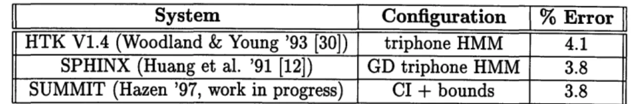
The Resource Management task is a useful framework for experimentation for two main reasons: first, it is a reasonably realistic simulation of the sorts of tasks we hope to accomplish with speech recognition; and second, as a result of annual DARPA evaluations, many papers have been published regarding performance on the task, including the gains reported by various systems as a result of incorporating context-dependent models [18, 15]. (See Table 3-1.)

The data in the Resource Management corpus are divided into separate sets for training and testing. Standard practice is to train on a 109-speaker training set,

'For example, "How many vessels are in Indian ocean?" and, for the fricative inclined, "Does sassafras have the largest fuel capacity of all Siberian Sea submarines?"

(29)

System Configuration I% Error

HTK V1.4 (Woodland & Young '93 [30]) triphone HMM 4.1 SPHINX (Huang et al. '91 [12]) GD triphone HMM 3.8 SUMMIT (Hazen '97, work in progress) CI + bounds 3.8

Table 3-1: The best results in the literature published for Resource Management's Feb. 1989 evaluation. (The error rates of 3.8% are actually for a slightly different, but harder test set.)

which I will call train109. This set contains a total of 3990 utterances, 2880 of which are from 72 speakers (40 utterances per speaker) and 1110 of which are from the remaining 37 speakers (30 utterances per speaker). Each speaker also recorded two "speaker-adaptation" utterances, which are not included in the training set. 78 of the speakers are male, and 31 are female.

The development test data used in the experiments described in this thesis are the data released for official evaluation purposes in February of 1989 (test89). The data consist of 300 utterances from 10 speakers, none of which is represented in the training data.

3.3 The Baseline Configuration

The baseline system classifies segments into one of 60 context-independent classes, corresponding to the units used to transcribe the TIMIT database [6], with the ex-ception of /eng/. The majority of the experiments described in this thesis involve subdividing these classes into several according to context. Otherwise, in most cases, the configuration of the system remains as described below.

The measurements used throughout this thesis are 39 averages and derivatives of MFCC values across various portions of the segment, plus the log of the duration of the segment. They are due to Muzumdar [20] and are described more exactly in Appendix A. The acoustic models are mixtures of diagonal Gaussian models, with a maximum of 30 mixtures per model and a minimum of 25 training tokens per mixture.2

In the case of the 60 context-independent classes, all but three (em, en, and zh) have sufficient training data to create all 30 mixtures. In the case of context-dependent models, very rarely does the number of mixtures approach the upper bound.

The language model is the bigram representation of the word-pair grammar, as described in Appendix B. This language model has a test-set perplexity of 62.26 on the 1989 evaluation set. The pronunciation network is created automatically by the application of rules to the baseform pronunciations for each word. There are no

2

That is, the number of mixtures used to represent a class is either 30 or the number of mixtures possible with 25 tokens per mixture, whichever is smaller.

(30)

weights on arcs of the pronunciation network, and so all paths through the network are assigned equal likelihood.

The Viterbi search and the A* search are both characterized by pruning thresh-olds. Typically, the Viterbi threshold is fixed at 15.0 and the A* threshold at 30.0. Increasing either threshold decreases the amount of pruning, increases computation cost, and (usually) improves performance. The values presented here are used because they provide sufficient pruning to approach real-time performance, without sacrificing a great deal of accuracy.

The recognizer includes a variety of other configurable parameters, but these are held constant throughout the thesis and do not warrant discussion here.

3.4 Baseline Performance

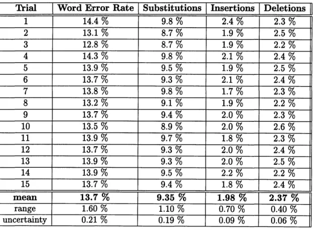
Most of the experiments performed in this thesis evaluate models trained on the 109-speaker training set and tested on the 10-109-speaker 1989 evaluation set. As discussed in Appendix C, in order to accurately assess the performance of the system, it is necessary to run multiple trials. In the following experiment, 15 sets of context-independent models were trained on the 109-speaker training set. Each was evaluated on the 1989 test-set, yielding an average word error rate of 13.7%.

Trial Word Error Rate Substitutions Insertions Deletions

1 14.4 % 9.8 % 2.4 % 2.3 % 2 13.1 % 8.7 % 1.9 % 2.5 % 3 12.8 % 8.7 % 1.9 % 2.2 % 4 14.3 % 9.8 % 2.1 % 2.4 % 5 13.9 % 9.5 % 1.9 % 2.5 % 6 13.7 % 9.3 % 2.1 % 2.4 % 7 13.8 % 9.8 % 1.7 % 2.3 % 8 13.2 % 9.1% 1.9 % 2.2 % 9 13.7 % 9.4 % 2.0 % 2.3 % 10 13.5 % 8.9 % 2.0 % 2.6 % 11 13.9 % 9.7 % 1.8 % 2.3 % 12 13.7 % 9.3 % 2.0 % 2.4 % 13 13.9 % 9.3 % 2.0 % 2.5 % 14 13.9 % 9.5 % 2.2 % 2.2 % 15 13.7 % 9.4 % 1.8 % 2.4 % mean 13.7 % 9.35 % 1.98 % 2.37 % range 1.60 % 1.10 % 0.70 % 0.40 % uncertainty 0.21 % 0.19 % 0.09 % 0.06 %

(31)

The word error rate is the sum of the substitutions, insertions, and deletions. The uncertainty in the measurement of the word error rate is calculated as described in Appendix C. In this case, for example, if one were to perform an infinite number of experiments, the word error rate averaged over all experiments would differ from 13.70% by more than 0.21% with a probability of 0.05. The range of possible results, however, is quite large (1.6%), clearly demonstrating the necessity of performing multiple experiments3.

Note that the results presented here are not competitive with those published in the literature (Table 3-1). The reason is that the system presented above was designed not to maximize performance, but rather to provide a solid baseline with respect to which further enhancements can be evaluated. Performance can nominally be improved by increasing the number of measurements per segment, the number of mixtures per model, or the pruning thesholds of the Viterbi and A* searches. Futhermore, corrective training could be used to optimize weights on the arcs of the pronunciation network, and other parameters throughout the system could be tuned by hand. Doing so, however, would provide little benefit to the value of comparative experimentation and would be contrary to the goal of designing a system that keeps computational costs within the range acceptable in a real-time system.

3.5 N-best Performance

The strategy of re-scoring the hypotheses of the N-best list is worthless if the top N choices do not include the correct answer, or at least utterances that are "more" correct than the first choice. Furthermore, one would like to know what value of N should be used. Is the correct answer almost always within the top 10 hypotheses? Within the top 100? What is the word error rate that we could achieve if we could choose the best among the hypothesis from the N-best list?

An experiment was designed to answer these questions. The first step was to compute N-best lists of size N = 100 for each of the 300 utterances in the 1989 test set, using a set of models trained on the 109-speaker training set. Then, for each value of N between 1 and 100, two statistics were calculated:

1. the word error rate across all 300 utterances, where each utterance is represented by the best among the top N hypotheses, and

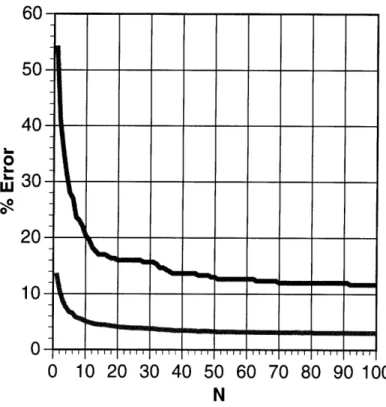
2. the sentence error rate on the same data; that is, the percent of utterances for which the correct answer is not included as one of the top N hypotheses. Figure 3-1 is a plot of the two statistics, which shows that a great deal of improve-ment is possible if the recognizer can learn to extract the best among the hypotheses represented in the N-best list. (Table 3-3 gives the exact values.) In some ways, this problem is much simpler than the original problem presented to the recognizer, due

3

All results published in this thesis are calculated as the average of several trials (usually 15), and the word error rate is typically accurate to within 0.25%

(32)

5 0_O 2 1 0 10 20 30 40 50 60 70 80 90 100 N

Figure 3-1: A plot of word and sentence error rate for an N-best list as a function of N. The upper curve is sentence error rate.

(33)

to the severely constrained search space embodied in the N-best list. In others, it is more difficult, since the differences between alternatives in the N-best list are often very slight, hinging on only a few segments of speech. But precisely because of the constraints imposed by the limited number of possibilities, the recognizer can afford to apply more computationally intensive techniques than during the first pass. One such technique is to use context-dependent acoustic models, the results of which are presented in the remaining chapters of this thesis.

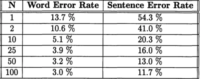
N I Word Error Rate Sentence Error Rate

1 13.7 % 54.3 % 2 10.6 % 41.0 % 10 5.1 % 20.3 % 25 3.9 % 16.0 % 50 3.2 % 13.0 % 100 3.0 % 11.7 %

Table 3-3: Word and sentence error rate on test89 as the length of the N-best list increases.

(34)

Chapter 4 Deleted Interpolation

4.1 Introduction

The training of context-dependent models is hindered by what is known as the "sparse data problem." That is, for very specific contexts, it is unlikely that there will be enough examples to train robust models; on the other hand, more general contexts lack the specificity that was the original goal of building context-dependent models. One solution to this tradeoff involves a technique called deleted interpolation [13], in which specific models are interpolated with more general models according to their performance on unseen data. This chapter introduces the concept of deleted inter-polation and describes its implementation within a segment-based speech recognition system.

4.2 Deleted Interpolation

Given a particular context-dependent model PCD(.) and its associated context-independent model Pc,(.), an interpolated model PDI(.) can be created as a linear combination of the two as follows [11]:

PDI(.) = APCD(.)+ (1 - A)PcI(.). (4.1) The goal is to interpolate the two component models such that the resulting model approximates the context-dependent model (A ; 1) when it is well-trained but "backs off" to the context-independent model (A 0 0) otherwise. Deleted interpolation is a technique for estimating the values of A by measuring the ability of each model to predict unseen data. The basic procedure is as follows [11]:

1. Partition the training set T into two disjoint sets, T1 and T2, such that T =

T1 u T2

-2. Train both the context-dependent model PCD(7T) (.) and the context-independent model PcI(71)(') on the data in T1.

Context-dependent modeling in a segment-based speech recognition system