HAL Id: halsde-00809138
https://hal.archives-ouvertes.fr/halsde-00809138
Submitted on 8 Apr 2013HAL is a multi-disciplinary open access archive for the deposit and dissemination of sci-entific research documents, whether they are pub-lished or not. The documents may come from teaching and research institutions in France or abroad, or from public or private research centers.
L’archive ouverte pluridisciplinaire HAL, est destinée au dépôt et à la diffusion de documents scientifiques de niveau recherche, publiés ou non, émanant des établissements d’enseignement et de recherche français ou étrangers, des laboratoires publics ou privés.
Simulation of morphogenetical gradients using a
minimal functional-structural plant model (FSPM)
Olivier Taugourdeau, Jean-François Barczi, Y. Caraglio
To cite this version:
Olivier Taugourdeau, Jean-François Barczi, Y. Caraglio. Simulation of morphogenetical gradients using a minimal functional-structural plant model (FSPM). Kang, M. Z.; Dumont, Y.; Guo, Y. Plant growth modeling, simulation, visualization and applications. Proceedings PMA12 : The Fourth International Symposium on Plant Growth Modeling, Simulation, Visualization and Applications, Shanghai, China, 31 October-3 November 2012, IEEE Press, pp.379-387, 2012, 978-1-4673-0068-1. �halsde-00809138�
Simulation of morphogenetical gradients using
a minimal Functional-Structural Plant Model (FSPM)
O TaugourdeauUniversity of Montpellier II – UMR AMAP F34000 Montpellier, France
JF Barczi, Y Caraglio CIRAD – UMR AMAP F34000 Montpellier, France Corresponding author: [email protected] Abstract—Context: Architectural studies highlight recurrent
morphogenetical gradients that are observed on some tree species. These morphogenetical gradients are linked to morphological trends among successive shoots throughout plant structure and ontogeny. This study aims at testing a potential origin of these gradients as the complex result of some core plant functions. It will be achieved through a minimalist mathematical modelling approach.
Methods: DRAFt is a discrete modelling approach at yearly step that benefits from a system of few mechanistic equations which attempts to simultaneously describe tree development (primary and secondary growth and branching) and functioning (assimilation and carbon partitioning). This FSPM aims at deeply interlacing both tree development and functioning using a formulation that keeps accuracy with knowledge about trees. DRAFt was implemented in AmapStudio for 3D simulations and outputs extractions. Main results: DRAFt succeeds in providing realistic trends with respect to morphogenetical gradients (tree base effect and axes drift). Different tree forms were simulated driven by input parameter values variations, which emphasize an effective model sensitivity. DRAFt consists in a 6 parameters system of equations which is minimalist compared to other previous more complex mechanistic FSPM.
Conclusion and perspectives: This results are consistent with the idea that some morphological gradients are an emergence of few basic tree functions. Based on this generalist and simple core, some other biological processes may be plugged (apex mortality, sexuality position) depending on the accuracy to the biological question that is assessed. The minimalist formulation provides a mathematical framework that facilitates both further mathematical and computational studies. Moreover it would be interesting to be able to fit DRAFt parameters with real measurements and to carry on a meticulous sensitivity analysis of DRAFt behaviour.
Keywords-component; Plant architecture; Functional-Structural Plant Models; Plant Growth; Plant Form; Trees; Minimal Mathematical Modelling
Abbreviations; SAM:Shoot Apical Meristem; Gu:Growth unit;
I. INTRODUCTION
Among living organisms plants show an iterative and modular development [1] that may span several decades and that results in a strongly organized growing structure. Pioneer works of Hallé & Oldeman [2], aims at describing plant form, structure and ontogeny according to a dynamic, multilevel and comprehensive approach [3]. The resulting “architectural analysis” aims at identifying the expression of endogenous processes and their modulation due to external influences that generates plant structure during its development.
One of the main results of this approach consists in the identification of generic morphological trends in trees ontogeny named morphogenetical gradients [3, 4]: the first one is the base effect (i.e. the increasing size of successive shoots produced by a juvenile stem apical meristem); the second one is the drift (i.e. the decreasing size of successive shoots produced by an ageing meristem); and at last the lateral production vigour gradient along a shoot.
One of the hot topics in plant architecture studies is to identify which among the endogenous processes are the causes of the observed morphological trends and to establish the functional link between them [5–8]. Base effect and drift may be assessed at different scale level. At stand scale, the biomass increase variation may be related to base effect on young stands, and drift to explain the reduction of biomass increase on mature stands [9]. At tree scale, the base effect may be linked with the increasing assimilation capacity according to tree size (e.g. total leaf area and root surface). Drift may be linked with a functional balance strategy that leads to a growth reduction, due to hydraulic constraints or structure self-maintaining costs for instance [9]. Finally, at shoot scale, meristems are the places where growth takes place and that set up plant structure development [3].
Shoot Apical Meristems (SAM) express primary growth (organogenesis and extension) and show base effect and drift gradients on the successive Growth Units (“Gu”: stem portion that is produced by an apical meristem during an uninterrupted extension period) that they set up along axes. Axillary meristems are expressed along Gu and are the origin of new lateral axes (branching process). Successive axillary meristems along bearer Gu may show vigour gradient [3] ,most of the time axillary meristems borne at the top of bearer Gu are the more vigourous. Finally, cambium which is a secondary meristem, produces secondary tissues (e.g.
wood) mainly aimed at mechanical, storage and hydraulic purposes.
Meristems activity mainly relies on resources intake (e.g. non structural carbohydrate) provided by leaf photosynthesis and transferred through hydraulic network mapped on tree structure [10].
The aim of this study is to build a minimal mathematical model that mimics growth and development of the tree aerial part based on carbon allocation (i.e. root system and underground stems contributions will not be considered). This model, called DRAFt (Demand, Resource, Architecture and Functioning at discrete time), will include some well-known core mechanistic processes which reflect endogenous processes [11]. Simulation of DRAFt should produce numerical plant architectures (growing set of Gus topologically organized and characterized by their size and mass) where base effect and drift are easy to measure, thus allowing to test if morphogenetical gradients may emerge from a small set of modeled endogenous processes.
Using modelling to simulate these emerging gradients may allow to assess the tree architecture diversity considering the trade-off between structure and function. A minimalist approach was chosen in order to allow a mathematical formalism which provides some numerical tools to study the model sensitivity and the system behavior. A minimal mathematical modelling approach has been considered to allow both theoretical and numerical studies. In this work we present a rough numerical study of the system behavior. The theoretical study will be developed in a forthcoming work.
II. MATERIALSAND METHODS
A. Modelling formalism
DRAFt is defined as a recurrence relation with an increment reflecting a regular constant time-step corresponding to the time between two successive shoots. Let Vt be the set of state variables that describes the tree at
iteration t. This explicitly takes into account the role of the structure itself on its future state. The evolution of Vt is
described by the following iteration equation:
V
t + 1=
f (V
t)
(1)The choice of discrete time formalism is a relevant scale for trees with a rhythmic growth that generates shoots and rings periodically (e.g. main tree species in temperate zones). We assume that a growth simulation at step t+1 only depends on the state variable values at iteration t. This choice was made for purposes of simplification. Behaviors that depends on delayed processes (epicormic meristems break, reserve use...) would require a more complex model like:
V
t + 1=
f (V
t,V
t −1, ...)
Furthermore a continuous time modelling (i.e. set of partial differential equations) may bring a greater biological
accuracy inducing at the same time a possible difficulty in finding a solution.
V =f (t)
f in equation (1) is a system of equations that will be described throughout the next paragraphs with a set of input parameters that are listed in Table 1.
Vector Vt consists of a set of variables that describes the tree and each Gu within it. Names and descriptions of these variables are listed in Table 1.
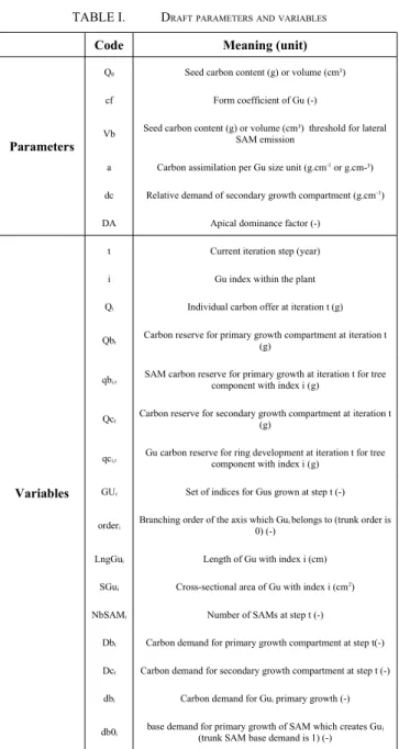
TABLE I. DRAFTPARAMETERSANDVARIABLES Code Meaning (unit)
Parameters
Q0 Seed carbon content (g) or volume (cm³)
cf Form coefficient of Gu (-)
Vb Seed carbon content (g) or volume (cm³) threshold for lateral SAM emission a Carbon assimilation per Gu size unit (g.cm-1 or g.cm-³)
dc Relative demand of secondary growth compartment (g.cm-1)
DA Apical dominance factor (-)
Variables
t Current iteration step (year) i Gu index within the plant Qt Individual carbon offer at iteration t (g)
Qbt Carbon reserve for primary growth compartment at iteration t (g)
qbi,t SAM carbon reserve for primary growth at iteration t for tree component with index i (g)
Qct Carbon reserve for secondary growth compartment at iteration t (g)
qci,t Gu carbon reserve for ring development at iteration t for tree component with index i (g)
GUt Set of indices for Gus grown at step t (-)
orderi Branching order of the axis which Gu0) (-) i belongs to (trunk order is
LngGui Length of Gu with index i (cm)
SGui Cross-sectional area of Gu with index i (cm2)
NbSAMt Number of SAMs at step t (-)
Dbt Carbon demand for primary growth compartment at step t(-)
Dct Carbon demand for secondary growth compartment at step t (-)
dbi Carbon demand for Gui primary growth (-)
B. DRAFt components and their sequence
DRAFt simulation begins with an initial state (i.e. the seed), that consists in an initial SAM and an initial pool of carbon (Q0). It then loops for a given number of iteration (T).
Model proposed in equation (1) at iteration t is divided in 6 successive substeps, each of them reflecting a particular endogenous process and written as an equation:
1. Gu growth based on carbon allocation performed in previous iteration
2. Branching: new SAMs added on Gu 3. Carbon assimilation by Gu
4. Carbon allocation to primary and secondary growth (compartment scale)
5. Rings growth at Gu scale based on carbon allocation to secondary growth
6. Carbon allocation to each SAM based on carbon allocation to primary growth
Our discrete iterative formalism imposes to order the 6 endogenous processes in a particular sequence according to biological constraints (e.g. ring allocation must be computed before SAM allocation since SAM demands may depend on rings cross-sectional area). It is worth to notice that this choice would not have to be done if a continuous modelling were applied. For instance it does not integrate any secondary growth during bud break [12]. Moreover, each SAM builds one Gu per iteration with carbon intake based on the previous iteration assimilation, which describes species with monocyclic preformed shoots [3]. Each Gu builds one new layer (i.e. tree ring, secondary growth) per iteration with carbon intake based on current iteration assimilation [12].
It is a carbon based model which does not take into account any effect of nitrogen or water on growth, and does not include any functional reserve compartment.
It is important to notice that every new SAM grows (i.e. no dormancy) with one iteration delay (i.e. one-year delayed branching) and there is no allocation to the reproduction compartment.
The following sections will describe each of the six substeps with the corresponding hypotheses we have made and the associated modelling choices.
C. Substep 1: Gu growth
This substep deals with giving dimensions to newly created Gus. Gu volume and dimensions (i.e. length and diameter) are directly inferred from the carbon allocation to SAMs which takes place at step 6 of the previous iteration (or from the seed at first iteration). Assuming that biomass carbon volumetric concentration remains constant across all plant components, we write that a carbon unit allocation (q) is equivalent to a biomass unit volume (v).
v=q
(2)Let qi,t be the total carbon allocated to Gui until iteration
t. It consists in a primary growth carbon allocated to the corresponding building SAM at step 6 of the previous
iteration (qbi) and the sum of secondary growths carbon
allocated to Gui throughout time (qci,j):
q
i, t=
qb
i+
∑
j=1 t
qc
i , j (3)For a simplification purpose, we assume that Gus are cylinders with a length-diameter ratio (cf parameter) that remains constant according to an allometric relationship to Gu volume.
LngGu
i=
√
34∗cf
2
π
∗
qb
i (4)(n.b. Gu length is fixed at Gu birth time and remains constant)
SGu
i ,t=
q
i , tLngGu
i (5)These assumptions exclude any shoot specialization within the simulated tree and throughout the tree ontogeny [13].
D. Substep 2: Branching, new SAMs added on Gu
This substep deals with the birth of new lateral SAMs borne by newly created Gus. We assume that the number of lateral branches is proportional to Gu volume (Vb parameter) which is commonly observed on trees [14].
NbSAM
t + 1=
NbSAM
t+
∑
i∈GUt+ 1
trunc(
qb
iVb
)
(6)
This assumption excludes any shoot specialization within the tree and throughout the tree ontogeny [e.g between short and long shoots, 13]. Moreover, all SAMs remain alive during tree growth simulation, which means no apical mortality (i.e. monopodial growth) and no self-pruning.
E. Substep 3: Carbon assimilation by Gu
This substep deals with carbon assimilation due to photosynthesis. We assume that only Gus created at iteration t can assimilate carbon. We also assume that the tree carbon assimilation is proportional (parameter a) to the sum of current Gus size: Aiba and Nakashizura [15] show the strong relationship (R² = 0,84) between tree leaf area and the net production of the plant and we can assume that the tree leaf area is closely related to the cumulated length of current year shoots [e.g. 16].
Q
t=
a∗
∑
i ∈GUt
LngGu
iThese assumptions exclude evergreen species and avoid any self-shading or conduction limits considerations [17].
F. Substep 4: Carbon allocation at compartment scale
This substep deals with carbon partitioning between two main compartments (primary and secondary growth). We assume that assimilated carbon is allocated according to common pool hypothesis and sink/source balance [18]. At this step the carbon is split between a global primary growth compartment and a global secondary growth compartment. Allocation to individual Gus for secondary growth and to individual SAMs for primary growth will be processed respectively at step 5 and 6.
Two possibilities were tested to compute global primary growth demand (Dbt). The first one is related to the number
of SAMs:
Db
t=
NbSAM
t (8a)The second one includes the apical dominance (parameter DA) and branching order. The demand of a Gu is computed as an exponential function of its branching order.
Db
t=
∑
i ∈GUt+ 1
DA
orderi(8b)
This modelling intends to include the branch hierarchy [3] into the carbon balance between primary and secondary growth.
Similarly, two possibilities were tested to compute the global secondary growth demand (Dct). In both cases, the
parameter dc rates Dct with respects to Dbt. The first one is
related to the sum of all Gu lengths.
Dc
t=
dc∗
∑
i ∈Plant
LngGu
i(9a)
The second one corresponds to the sum of all path lengths from tree apical ends to the tree base. Let Pathi be the
list of indices from the tree base to Gui.
Dc
t=
dc∗
∑
i ∈GUt(
DA
orderi∗
∑
j ∈PathiLngGu
j)
(9b) This modelling is equivalent to the pipe model [19]. Carbon is split between primary growth compartment (Qbt) and secondary growth compartment (Qct) according toa demand ratio.
Qb
t=
Q
tDb
t+
Dc
t∗
Db
tQc
t=
Q
tDb
t+
Dc
t∗
Dc
t (10)These assumptions exclude any preferential allocation, neither due to proximity [18] nor due to growth strategy [20]. No references were found about the biomass partitioning between primary and secondary growth at whole-tree scale. This leads us to propose these simple modelling choices: models proposed in 8a and 9a are linked to the number of components within the tree; while models proposed in 8b and 9b try to include some biological knowledge coming from each process that has been studied independently.
G. Substep 5: Ring development
This substep deals with secondary carbon partitioning along axes. We assume that Gu secondary growth allocation (qci,t) is achieved according to the pipe model [19] applied on
Qct so that everywhere in the tree current ring surface is
equal to sum of surface of current borne rings. Equation (3) gives the new Gu volume sequence.
H. Substep 6: SAM allocation
This substep deals with primary carbon partitioning among all SAMs. We assume that the SAM carbon allocation is computed according to SAMs demand ratio. Let dbi and qbi, be respectively, the demand and the carbon
allocated to a SAM at iteration t to create Gui at iteration t+1.
for i∈GU
t +1:
qb
i=
db
i∑
j ∈GUt +1
db
j∗
Qb
t (11)Two ways were tested to compute the individual primary growth demand (dbi). The first one includes axis branching
order (orderi) and apical dominance (parameter DA).
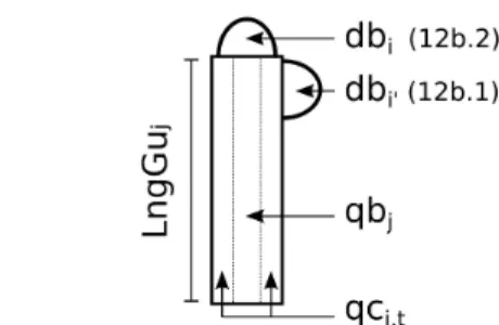
Figure 1. Gu and SAMs sketch explaining topological relationship used in 12b.1 and 12b.2. i and i' are respectively the apical and lateral indices
of productions borne by Gu with index j. qbj corresponds to primary
growth carbon allocation, at step 1 of current iteration, that determines Gu length (LngGuj) and qcj,t corresponds to the first secondary growth carbon
db
i=
DA
orderi (12a)This assumption makes equal every Gu that was born at the same iteration and belonging to the same branching order. This means that, at a given iteration, SAM's demand is independent from architectural position except branching order (e.g. vertical position within the crown or position along axes). Moreover it is a simple modelling useful for further mathematical study.
The second one tries to improve this potential weakness for describing vigor gradient of lateral axes within the crown [21]. We introduce the concept of SAM “base demand” (db0) which is linked to all Gus that were created by a single SAM along an axis. This value is computed at SAM's birth time and corresponds to its initial demand. It is arbitrarily set to 1 for all Gus of the trunk and, for other axes, is computed according to bearer Gu base demand (Fig. 1), apical dominance (parameter DA) and bearer Gu's ring cross-sectional area to take conduction features into account [18].
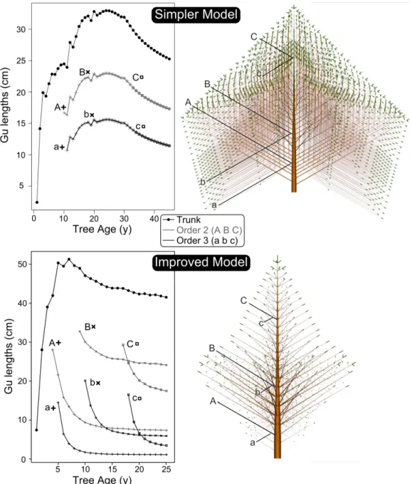
Figure 2. Simulation of successive Gu lengths along the trunk and three branches order 2 (uppercase letters) and order 3 (lowercase letters).
Simpler model: simulation based on modelling options 8a, 9a and 12a, parameter values: Q0=0.8; a=2; Vb=20; cf=20; dc=0.01; DA=0.4; tree age=45;
Improved model: simulation based on modelling options 8b, 9b and 12b, parameter values: Q0=0.8; a=6; Vb=25; cf=20; dc=0.004; DA=0.3; tree age=25.
Let j be the index of the Gu that bears the SAMwhich will create Gui.
for new SAMs at iteration t:
db
i=
db0
i=
DA∗db0
j∗
qc
j ,tLngGu
j (12b.1)for other SAMs at iteration t:
db
i=
db0
j∗
qc
j , tLngGu
j (12b.2)These models lack in generating lateral axes vigor gradient along a Gu: all axes borne by the same Gu behave exactly in the same way.
I. Implementation
An implementation of DRAFt was achieved using Xplo software from the AMAPstudio free-to-use package (http://amapstudio.cirad.fr). It is written in Java and generates the corresponding ArchiTree topology (an improved implementation of MTG datat structure, [22]) throughout time with each Gu having its own computed length and diameter. A very rough branching angle rule enables building a simple 3D shape. Xplo allows to draw it and also to make virtual selective measurements on simulated trees. Both outputs will be used into the Results section.
The use of this software environment made it easy to test the model sensitivity to each parameter and to explore the output solutions set that DRAFt can provide. The sets of parameters that are used in the Results section try to emphasize the goal of DRAFt model as announced in the Introduction section.
III. RESULTS
A. Morphogenetical gradients emergence
Keeping in mind that we want DRAFt to show some morphogenetical gradients (base effect and drift), two modelling choices were simulated: a model driven by a simplified compartment carbon allocation (8a and 9a) and SAM demand (12a); and a second one with improved modelling options (8b, 9b and 12b). They will be called the Simpler Model and the Improved Model respectively.
Considering Gu lengths (Fig. 2, right), simulations of the Simpler Model clearly shows a drift and a base effect at tree scale. Combined with branching order hierarchy, a maximal branching order emerges. Nevertheless, we observe : (i)a homothetic pattern between each branching order: laterals axes did not show any drift during trunk base effect; (ii) a self-similarity within each branching order: at a given iteration, all Gus belonging to the same branching order share the same quantitative properties.
Compared to the tree crown shape generated by the Simpler Model (Fig. 2 upper right), the Improved Model generates a more realistic tree crown shape (Fig. 2 lower right) and good quantitative properties (i.e. branching order hierarchy combined to vigor gradients along bearer).
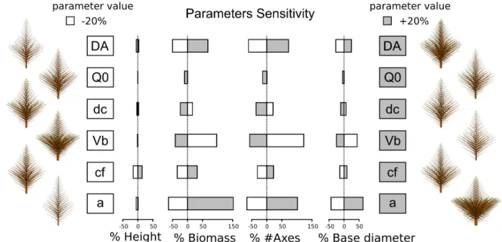
Figure 3. Effect of parameters variations (+/- 20%) on various simulated trees properties. The relative variations of tree height, biomass, number of axes and base diameter are shown for a relative variation of 20% of the corresponding parameter. A single parameter value is changed for each simulation while the modelling choices and other reference parameter values remain the same as in Figure 2. bottom (i.e. Improved Model: Q0=0.8; a=6; Vb=25;
cf=20; dc=0.004; DA=0.3; tree age=25). The corresponding simulated trees mock-ups are provided on the edges, near to the corresponding parameter
B. Sensitivity analysis
We choose to present some relevant output variables responses (tree height, total biomass, number of axes and base diameter) with respect to input parameters variations (Fig. 3). The choice of the output variables was performed to quantify complementary aspects of the tree structure. In order to make it easier to interpret variations, we decided to change only one parameter at a time for each simulation for a +/- 20% shift around a reference parameters set of values (the same used to provide Fig. 2). We used the Improved Model to perform this local sensitivity analysis.
At first sight, the results clearly highlight asymmetric responses of output variables to a symmetric shift of input parameters value. We also notice that all presented variables show the same variation direction for a given row into Fig. 3.
Within the chosen parameter variation range around mean values, we observed that Q0, dc and cf seem to have a
smaller quantitative influence on variables than DA, Vb and
a (Fig. 3). The Improved Model is not very sensitive to Q0
variations which were expected from the modelling assumptions.
Compared with other output variables, tree height seems to remain quite stable. It can be an emergent property of the Improved Model that is worth further studies. We could also notice that against intuitive forecast, secondary growth demand increase (dc) have a negative influence on the trunks base diameter and increase of trunk dominance (i.e. DA decrease) have a small but negative effect on tree height.
IV. DISCUSSION
A. Emerging properties of plants functioning
Using the same general scheme (i.e. an iterative development loop split into 6 substeps) and based on biological assumptions, we proposed two different modelling choices that both show emergent ontogenetic trends. Depending on the modelling choices, DRAFt successes in expressing base effect and drift at tree level (Simpler Model) and also at axes scale (Improved Model). In fact, Improved Model simulation is able to show asynchronous lateral axes drift compared to trunk combined with axes gradient within the crown, which fits with observed data on real trees [21]. It allows to expect that a part of morphogenetical gradients directly emerge from few core physiological processes (carbon assimilation and partitioning between primary and secondary growth and unbalanced partitioning between SAMs), which is not a so obvious consideration and gives way to further studies about their influence on plant architecture diversity.
These results were obtained with a model based on only 6 input parameter values, which is a rather parsimonious parametrization among other Functional-Structural Plant Models [i.e. FSPM, 23] and offers perspectives for numerical formal analysis (e.g. asymptotic behavior and mathematical explanations of model outputs) and further modelling works.
B. Limits due to DRAFt modelling choices
Each of the 6 parameters are assumed to remain constant throughout time and across plant, despite biological knowledge about ontogenetic shift of shoot form [13], photosynthetic capacity [24], or apical dominance [25] for instance.
All lateral axes borne by the same Gu remain equal during the simulation, despite biological knowledge about vigor gradients [26] or asymmetric allocation depending of axis local environment [20].
For a simplification purpose, we chose to express the tree carbon assimilation as a function of cumulated new Gu lengths at each iteration step, which avoids complex light interception computing, but may be an oversimplification according to biological knowledge [27].
A critical modelling point was to decide how to split carbon between primary and secondary growth compartments. This difficulty relies on the lack of data about this topic to our knowledge.
C. Toward DRAFt calibration according to real datasets
Some measurements made on tree structures (e.g. Gu length and number of branches) can be carried out a
posteriori [i.e. retrospective analysis of growth, 21]. Thus
retrospective measurements of morphological traits combined with a relevant modelling may allow to infer the past functioning of the tree [28]. To do so, it is necessary to be able to estimate the parameters values that will optimize the simulated tree compared to the measurements (i.e. calibration).
In DRAFt, some of the parameters values may be directly linked to output variables that will be compared to measurements. It means that some parameters can be directly estimated from accurate measurements. For instance DA can be directly inferred from mean value of Gu lengths ratio according to equation (13).
DA=
qb
iqb
i'=
4∗cf
2π∗
LngGu
i3∗
π∗
LngGu
i '34∗cf
2DA=
(
LngGu
iLngGu
i ')
3 (13)cf. Fig. 1 for i and i' definition.
Q0 can be written as a function of cf and first trunk Gu
length (LngGu1):
Q0= 1
cf
2∗
π∗
LngGu
134
(14)Vb (threshold for new lateral SAM birth) can be written
as a function of cf and Gu lengths (LngGui) and
corresponding number of borne lateral axes (LatAxei) that
Vb=
qb
iLatAxe
i=
π∗
LngGu
i34∗cf
2∗
LatAxe
iVb=
1
cf
2∗
π∗
LngGu
i34∗LatAxe
i (15)As a result, only cf, a and dc has to be estimated by heuristic approach based on simulations. The measurement protocol should be defined in order to obtain a non ambiguous estimation of these three parameters: only one set of parameters should provide an optimal simulation according to measurements.
D. DRAFt formalism refinements
We assume that we have defined a core model that expresses relevant biological properties about tree structure and ontogeny (i.e. plant architecture). Based on that core and without changing it, other biological processes may be modelled.
For instance: reproduction, axes specialization (long vs. short shoot) or axes death may be driven according to threshold functions on some local or global state variables [29,30]. In order to control tree death, a life cost function may be added [31]. The lack of lateral axes vigor gradient may be solved by introducing refinements in SAM base demand computing according to SAM position along the bearer Gu [26].
It is important to notice that we have been focusing on aerial part modelling avoiding any root consideration. A global black-box root compartment or a detailed approach similar to aerial part may be included. This would allow to refine biomass production modelling according both to carbon and nitrogen assimilation [31].
E. Feedbacks between structure and function in DRAFt
Most of existing FSPMs couple a morphogenesis sub-model with a function sub-sub-model: functioning occurs on a given structure and morphogenesis takes functioning as an input[e.g. 32,33], the two processes occur in sequence and interact one after each other. DRAFt modelling and formalism deeply interlaces both aspects in such a way that it is impossible to split them into two isolated sub-models. An emerging question would be to identify each aspect for every DRAFt equations and parameters. For instance we already suspect that shoot allometry assumptions (cf) hide a strong link between structure (i.e. the dimensions of the shoots) and functioning (i.e. carbon assimilation).
As a summary, DRAFt offers a unique minimal formalism that deeply integrates tree structure and function. It shows emergent morphogenetical trends without any empirical constraint.
ACKNOWLEDGMENT
We would like to thank the members of the Amap team for their support and kind advices with special thanks to Y. Dumont, S. Griffon and N. Row. UMR AMAP is a joint research unit that associates CIRAD (UMR51), CNRS
(UMR5120), INRA (UMR931), IRD (R123) and Montpellier 2 University (UM27) France; http://amap.cirad.fr/.
REFERENCES
[1] J. Harper, B. Rosen, and J. White, " The growth and form of modular organism ", London: The Royal Society, 1986. [2] F. Hallé and R. A. A. Oldeman, Essai sur l’architecture et la
dynamique de croissance des arbres tropicaux. Paris: Masson,
1970.
[3] D. Barthélémy and Y. Caraglio, " Plant architecture: A dynamic, multilevel and comprehensive approach to plant form, structure and ontogeny ", Annals of Botany, vol. 99, no. 3, p. 375–407, mars 2007.
[4] D. Barthélémy, Y. Caraglio, and E. Costes, " Architecture, gradients morphogénétiques et âge physiologique chez les végétaux ", in Modélisation et simulation de l’architecture des
végétaux, J. Bouchon, P. de Reffye, et D. Barthélémy, Éd.
Science Update, INRA éditions, 1997, p. 89–136.
[5] P.-H. Cournède, A. Mathieu, F. Houllier, D. Barthélémy, and P. de Reffye, " Computing Competition for Light in the GREENLAB Model of Plant Growth: A Contribution to the Study of the Effects of Density on Resource Acquisition and Architectural Development ", Ann Bot, vol. 101, no. 8, p. 1207–1219, mai 2008.
[6] R. W. Pearcy, H. Muraoka, and F. Valladares, " Crown architecture in sun and shade environments: assessing function and trade-offs with a three-dimensional simulation model ",
New Phytologist, vol. 166, no. 3, p. 791–800, juin 2005. [7] K. Yoshimura, " Hydraulic function contributes to the
variation in shoot morphology within the crown in Quercus
crispula ", Tree physiology, vol. 31, no. 7, p. 774–781, 2011. [8] M. G. Ryan, N. Phillips, and B. J. Bond, " The hydraulic
limitation hypothesis revisited ", Plant, Cell & Environment, vol. 29, no. 3, p. 367–381, mars 2006.
[9] P. Cruiziat, H. Cochard, and T. Améglio, " Hydraulic architecture of trees: main concepts and results ", Annals of
Forest Science, vol. 59, no. 7, p. 723–752, 2002.
[10] A. Lacointe, " Carbon allocation among tree organs: a review of basic processes and representation in functional-structural tree models ", Annals of Forest Science, vol. 57, no. 5, p. 521– 533, 2000.
[11] C. B. K. Rathgeber, S. Rossi, and J.-D. Bontemps, " Cambial activity related to tree size in a mature silver-fir plantation ",
Ann Bot, vol. 108, no. 3, p. 429–438, sept. 2011.
[12] E. Nicolini and B. Chanson, " The short shoot, an indicator of beech maturation (Fagus sylvatica L.) ", Canadian Journal of
Botany, vol. 77, no. 11, p. 1539–1550, nov. 1999.
[13] V. L. Gavrikov and O. P. Sekretenko, " Shoot-based three-dimensional model of young Scots pine growth ", Ecological
Modelling, vol. 88, no. 1?3, p. 183–193, juill. 1996.
[14] M. Aiba and T. Nakashizuka, " Growth properties of 16 non‐ pioneer rain forest tree species differing in sapling architecture ", Journal of Ecology, vol. 97, no. 5, p. 992–999, sept. 2009.
[15] A. Takenaka, " Structural variation in current-year shoots of broad-leaved evergreen tree saplings under forest canopies in warm temperate Japan ", Tree Physiol., vol. 17, no. 3, p. 205– 210, mars 1997.
[16] G. Koch, S. Sillett, G. Jennings, and S. Davis, " The limits to tree height ", Nature, vol. 428, no. 6985, p. 851–854, avr. 2004. [17] L. F. Marcelis and E. Heuvelink, " Concepts of modelling
Functional-structural Plant Modelling in Crop Production. Springer, Dordrecht p. 103–111, févr. 2007.
[18] H. Cochard, S. Coste, B. Chanson, J.-M. Guehl, and E. Nicolini, " Hydraulic architecture correlates with bud organogenesis and primary shoot growth in beech (Fagus
sylvatica) ", Tree Physiology, vol. 25, p. 1545–1552, 2005.
[19] K. Shinozaki, K. Yoda, K. Hozumi, and T. Kira, " A quantitative analysis of plant form-the pipe model theory: I. Basic Analyses ", Jap. J. Ecol., vol. 14, no. 3, p. 97–105, 1964. [20] K. Kawamura, " A conceptual framework for the study of
modular responses to local environmental heterogeneity within the plant crown and a review of related concepts ", Ecol Res, vol. 25, no. 4, p. 733–744, janv. 2010.
[21] O. Taugourdeau, J. Dauzat, S. Griffon, S. Sabatier, Y. Caraglio, and D. Barthélémy, " Retrospective analysis of tree architecture in silver fir (Abies alba Mill.): ontogenetic trends and responses to environmental variability ", Annals of Forest
Science, 2012.
[22] C. Godin and Y. Caraglio, " A multiscale model of plant topological structures ", Journal of Theoretical Biology, vol. 191, no. 1, p. 1–46, mars 1998.
[23] T. M. DeJong, D. Da Silva, J. Vos, and A. J. Escobar-Gutierrez, " Using functional-structural plant models to study, understand and integrate plant development and ecophysiology ", Ann. Bot., vol. 108, no. 6, p. 987–989, oct. 2011.
[24] S. Coste, J. Roggy, L. Garraud, P. Heuret, E. Nicolini, and E. Dreyer, " Does ontogeny modulate irradiance-elicited plasticity of leaf traits in saplings of rain-forest tree species? A test with Dicorynia guianensis and Tachigali melinonii (Fabaceae, Caesalpinioideae) ", Annals of Forest Science, vol. 66, no. 7, nov. 2009.
[25] Y. Claveau, C. Messier, P. G. Comeau, and K. D. Coates, " Growth and crown morphological responses of boreal conifer seedlings and saplings with contrasting shade tolerance to a gradient of light and height ", Canadian Journal of Forest
Research, vol. 32, p. 458–468, mars 2002.
[26] S. Sabatier and D. Barthélémy, " Bud structure in relation to shoot morphology and position on the vegetative annual shoots of Juglans regia L. ", Annals of Botany, no. 87, p. 1–7, 2001. [27] J. Dauzat, P. Clouvel, D. Luquet, and P. Martin, " Using
virtual plants to analyse the light-foraging efficiency of a low-density cotton crop ", Annals of Botany, vol. 101, no. 8, p. 1153–1166, mai 2008.
[28] F. H. Schweingruber, Tree rings and environment:
dendroecology. Switzerland: Paul Haupt AG Bern, 1996.
[29] V. Letort, P. Heuret, P.-C. Zalamea, E. Nicolini, and P. de Reffye, " Analysis of Cecropia sciadophylla Morphogenesis Based on a Sink-Source Dynamic Model ", in 2009 Third
International Symposium on Plant Growth modelling, Simulation, Visualization and Applications (PMA), 2009, p.
10–17.
[30] S. Bornhofen, " Emergence de dynamiques évolutionnaires dans une approche multi-agents de plantes virtuelles, PhD thesis ", 2008.
[31] S. Bornhofen and C. Lattaud, " Competition and evolution in virtual plant communities: a new modelling approach ",
Natural Computing, vol. 8, no. 2, p. 349–385, juin 2008. [32] J. Perttunen, R. Sievanen, and E. Nikinmaa, " LIGNUM: a
model combining the structure and the functioning of trees ",
Ecological Modelling, vol. 108, no. 1-3, p. 189–198, 1998. [33] P. De Reffye and B. Hu, " Invited talk. Relevant qualitative
and quantitative choices for building an efficient dynamic plant growth model: GreenLab case ", Plant Growth