Publisher’s version / Version de l'éditeur:
Advanced Manufacturing: Polymer & Composites Science, 3, 1, pp. 32-41,
2017-04-26
READ THESE TERMS AND CONDITIONS CAREFULLY BEFORE USING THIS WEBSITE. https://nrc-publications.canada.ca/eng/copyright
Vous avez des questions? Nous pouvons vous aider. Pour communiquer directement avec un auteur, consultez la première page de la revue dans laquelle son article a été publié afin de trouver ses coordonnées. Si vous n’arrivez pas à les repérer, communiquez avec nous à [email protected].
Questions? Contact the NRC Publications Archive team at
[email protected]. If you wish to email the authors directly, please see the first page of the publication for their contact information.
NRC Publications Archive
Archives des publications du CNRC
This publication could be one of several versions: author’s original, accepted manuscript or the publisher’s version. / La version de cette publication peut être l’une des suivantes : la version prépublication de l’auteur, la version acceptée du manuscrit ou la version de l’éditeur.
For the publisher’s version, please access the DOI link below./ Pour consulter la version de l’éditeur, utilisez le lien DOI ci-dessous.
https://doi.org/10.1080/20550340.2017.1311094
Access and use of this website and the material on it are subject to the Terms and Conditions set forth at
A three-dimensional transient model for heat transfer in thermoplastic
composites during continuous resistance welding
Zammar, Imad; Huq, M. Saiful; Mantegh, Iraj; Yousefpour, Ali; Ahmadi,
Mojtaba
https://publications-cnrc.canada.ca/fra/droits
L’accès à ce site Web et l’utilisation de son contenu sont assujettis aux conditions présentées dans le site LISEZ CES CONDITIONS ATTENTIVEMENT AVANT D’UTILISER CE SITE WEB.
NRC Publications Record / Notice d'Archives des publications de CNRC:
https://nrc-publications.canada.ca/eng/view/object/?id=945b4463-733d-4eca-a3d2-0a2b96210494
https://publications-cnrc.canada.ca/fra/voir/objet/?id=945b4463-733d-4eca-a3d2-0a2b96210494
Full Terms & Conditions of access and use can be found at
http://www.tandfonline.com/action/journalInformation?journalCode=yadm20
ISSN: 2055-0340 (Print) 2055-0359 (Online) Journal homepage: http://www.tandfonline.com/loi/yadm20
A three-dimensional transient model for heat
transfer in thermoplastic composites during
continuous resistance welding
Imad Zammar, M. Saiful Huq, Iraj Mantegh, Ali Yousefpour & Mojtaba
Ahmadi
To cite this article:
Imad Zammar, M. Saiful Huq, Iraj Mantegh, Ali Yousefpour & Mojtaba Ahmadi
(2017) A three-dimensional transient model for heat transfer in thermoplastic composites during
continuous resistance welding, Advanced Manufacturing: Polymer & Composites Science, 3:1,
32-41, DOI: 10.1080/20550340.2017.1311094
To link to this article: http://dx.doi.org/10.1080/20550340.2017.1311094
© 2017 The Author(s). Published by Informa UK Limited, trading as Taylor & Francis Group
Published online: 26 Apr 2017.
Submit your article to this journal
Article views: 129
View related articles
32 DOI 10.1080/20550340.2017.1311094
© 2017 The Author(s). Published by Informa UK Limited, trading as Taylor & Francis Group.
This is an Open Access article distributed under the terms of the Creative Commons Attribution License (http://creativecommons.org/licenses/by/4.0/), which permits unrestricted use, distribution, and reproduction in any medium, provided the original work is properly cited.
Introduction
Thermoplastic composites (TPCs) have now come a long way as a structural material for high performance applications such as aerospace with the popularity primarily stemming from their higher strength-to-weight ratio than most metals.1,2
As an engineering material, TPCs are also characterized by high damage tolerance,3 re-processability,4 good fatigue
resistance, low storage cost, and ininite shelf life.5,6 With all
these attractive attributes, challenges still remain to manu-facture composite components in large-scale scenarios due to the high cost associated with complicated mold designs as well as the use of expensive machinery, such as an autoclave.
Consequently, the only viable method to make large or com-plex parts appears to be to mold the simple parts and join them together.7
Resistance welding, a kind of fusion bonding, is a wide-spread alternative process to mechanical fastening and adhesive bonding in joining TPCs. Nowadays, it is seen as one of the most promising techniques for joining thermo-plastic composite TPC laminates.5,8 The technique is based on
melting of a thermoplastic polymer at a joint interface using heat generated by resistive (Joule) heating of a conductive or heating element placed between the surfaces to be welded by circulating an electrical current through it while the joint is under applied pressure. The advantages usually attributed to resistance welding include fast processing time, little or no surface preparation, possibility of reprocessing if subsequent non-destructive evaluation reveals defects and possibility of
A three-dimensional transient model for heat
transfer in thermoplastic composites during
continuous resistance welding
Imad Zammar
1, M. Saiful Huq
2, Iraj Mantegh
3, Ali Yousefpour
3and Mojtaba Ahmadi
1,*1Mechanical and Aerospace Engineering Department, Carleton University, Ottawa, ON, Canada K2S 5B6
2Department of Mechatronic and Robotic Engineering, University Tun Hussein Onn Malaysia (UTHM), Johor, Malaysia 3National Research Council (NRC) Canada, Institute for Aerospace Studies, Montreal, CQ, Canada H3T 2B2
AbstractThe resistance welding technique for thermoplastic composites (TPCs) entails melting the TPC polymer at the joint interface using heat generated by resistive (Joule) heating of a conductive mesh or heating element placed between the surfaces to be welded. The continuous resistance welding (CRW) is an automated large-scale resistance welding technique that consists of a moving voltage source along the heating element creating a continuous weld along its path. This paper presents a transient model that is developed to predict the heat transfer in TPCs in all three dimensions during the CRW process. The model is finite element in nature and includes both the resistive and thermal conductivity behaviors of the material involved. The significance of this modeling
approach is that it captures the movement of the electrical connection, as well as the nonuniform distribution of the current and resistive heating along the length and width of the weld seam. The modeling results are compared with experimental data obtained by thermocouples and an infrared camera, and exhibit solid conformance for predicting the trend of variations in weld temperature.
Keywords Thermoplastic composites (TPCs), Resistance welding, Composite welding, Heat transfer, Finite element modeling (FEM)
Cite this article Imad Zammar, M. Saiful Huq, Iraj Mantegh, Ali Yousefpour and Mojtaba Ahmadi: Adv. Manuf.: Polym.
Compos. Sci., doi:10.1080/20550340.2017.1311094
Original Research Paper
*Corresponding author, email [email protected]
Received25 August 2016; accepted 6 March 2017
Advanced Manufacturing: Polymer & Composites Science 2017 VOL. 3 NO. 1
online control.9,10 Yet, in case of welding large joints, the
pro-cess of resistance welding is quite constrained, primarily by the high power and pressure requirements, if a direct scale-up is considered.8 A realistic alternative is to efectively break
down a large weld into smaller segments to be welded in sequence using an automated or controlled relative motion of the small-scale welding tool along the weld seam.9,11–13
Several studies attempts to model the heat transfer in TPCs in the resistance welding scenario with a view to study the associated process parameters, with most of them resorting to numerical modelling approach. A transient three-dimensional (3-D) numerical model (inite element modeling [FEM]) for resistance welding of CF/PEI lap shear joints was developed by Ageorges et al.14 The model considers orthotropic heat
con-duction and is able to predict melting and degradation times within close agreement with experimental data available in the literature. Jakobsen et al.15 developed a transient
two-di-mensional (2-D) FEM for resistance welding of APC-2 laminate. Anisotropic heat transfer is considered for double cantilever beam (DCB) specimens of an APC-2-laminate/PEEK-ilm sys-tem. Holmes and Gillespie16 developed 1-D and 2-D FEM for
large scale sequential resistance welding of APC-2 specimens with the objective of tuning welding parameters by assessing uniformity of the interface temperature through simulation. A 2-D FEM of the resistance welding of APC-2 lap shear spec-imens was developed by Xiao et al.17 Don et al.18 attempted
to use inite diference approach in developing 2-D models for the process heat transfer. Carbone and Langella19
devel-oped a numerical model using COMSOL Multiphisics user interface. The numerical prediction in all the later three stud-ies was used to study the process parameters for resistance welding. Alongside numerical modeling approaches, a hand-ful of the studies do resort to analytical modelling approach to study the heat transfer during resistance welding in TPCs. Mafezzoli et al.20,21 proposed a mathematical model to
pre-dict heat transfer (and the subsequent crystallinity level) for resistance welding of APC-2 laminates. The model proposed by Bastien and Gillespie22 is based on the healing theory of
amorphous polymers and was used to predict strength and toughness of joints as a function of non-isothermal process history. While all these studies attempt to model the process to an acceptable degree of accuracy, all of them were devel-oped considering a stationary heat source and as such are not suitable for large-scale welding scenario where the tool moves along the weld seam as in the case of the continuous resistance welding (CRW)12,13 (please see Section Continuous
thermoplastic resistance welding (CRW) for details).
Modeling the process using 3-D FEM approach can help the automation of large-scale welding in primarily two ways. Firstly, it can facilitate the study of the dynamics of temperature
at the weld interface and thus allow the efective tuning of the welding parameters. Secondly, it can be used as an observer (or to derive an observer) that would allow the estimation of the online temperature at any desired point within the physical dimension of the workpiece during the weld and thus avoid the requirement of any sensor to be placed or used, which may be a diicult task given a complicated weld setup which already covers the welding area, as in the case of CRW. Besides, it can potentially provide a visualization of some parameters that are diicult to determine experimentally. An example of this would be the distribution of the current along the length of the weld, and the weld zone temperature. Under these rea-sonings, a 3-D FEM was developed for a TPC in the CRW sce-nario using COMSOL Multiphysics inite element solver and is presented in this paper. This paper attempts to understand the heating phenomena that occur during the weld. The concept of preheating, and secondary heating are important aspects to the CRW process. CRW must take into account the heating that occurs before and after a section is welded to ensure suicient pressure is applied to form a proper weld. Insuicient knowl-edge of pre and post-heating could result in pressure being removed from the weld before solidiication has occurred. This paper represents this phenomenon, as well as the electrical current luctuation that is the root cause of the heating.
Continuous thermoplastic resistance
welding (CRW)
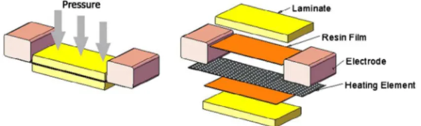
The process of resistance welding involves placing a conduc-tive implant, called the heating element between the two parts to be joined. A typical weld stack for the resistance welding process is shown in Fig. 1. Sandwiched between the two com-posite laminates is a stainless mesh – the heating element, with a neat resin ilm on either side of it. An electrical current is passed along the heating element by means of copper elec-trodes located at the ends of the stainless steel mesh causing its temperature to rise due to resistance heating following the Joule’s Law, which is a function of both the weld current (I) and electrical resistance (R) (Eq. (1)). The thermoplastic matrix starts to melt once the bond line temperature rises to a cer-tain point. Following the achievement of nominal melting, current is switched of and the joint is allowed to cool. The whole process takes place under adequate pressure to enable intimate contact between the laminate surfaces and promote molecular difusion in the interface. Since the heating element is diferent from the TPC, resin ilms, which are typically the same as the resin used in the laminate, are used to impregnate the heating element to achieve material compatibility on the molecular level after bonding.23
Figure 1 Thermoplastic resistance welding stack
Zammara et al. Three-dimensional transient model
Advanced Manufacturing: Polymer & Composites Science 2017 VOL. 3 NO. 1 34
Since a direct scale-up is not a feasible option for large scale manufacturing due to high power and pressure requirements, the CRW approach efectively brakes down a large weld into smaller segments or weld sections by implementing con-tinuous motion of the welding tip along the weld seam. Considering the fact that the performance and quality of the bonded joint are related directly to the weld interface ther-mal history,22 in the CRW, the continuous motion is in fact
used as the control input within a feedback control scheme to maintain a desired weld temperature, thereby ensuring a high quality bond.12,13 Furthermore, to prevent excessive
power drain and restrict the heating process more within the current weld section, the power inlet to the relatively long heating element is made up of electrically isolated copper blocks, instead of a pair of continuous copper strips.9,11–13 The
arrangement essentially enables continuous repetition of the static resistance welding process described above on a weld stack similar to that of the a static process (Fig. 1), except that the overall length of the weld seam is longer and the pair of copper strips on either side of the weld stack acting as the power inlet is made up of electrically isolated copper blocks.
The technique requires a moving power source to supply the energy to subsequent weld sections, as well as a moving pressure source to continuously apply pressure to the weld sections for the proper amount of time. All these requirements (1)
H = I2×R call for a specialized custom built end-efector and was built
accordingly at the Aerospace Manufacturing Technology Centre (AMTC), a division of the Institute for Aerospace Research (IAR) at the National Research Council (NRC). The overall current setup involves intelligent feedback control of the weld temperature with weld speed as the control input using an industrial robot – KUKA KR 210 equipped with the custom built end-efector (Fig. 2).
Methods
COMSOL Multiphysics software is a multiphysics FEM soft-ware allowing coupled problems such as heat and strain to be solved dynamically. It uses a simple and intuitive inter-face, creates meshes automatically, has most common mate-rial properties, and allows deining custom values based on functions, or experimental data, as well as easy geometrical data input and revisions. Therefore, COMSOL was used as a software ofering ease of use in fast prototyping of complex nature. Two types of physics, viz. “Conductive Media DC” and “General Heat Transfer”, were used to model the process. The irst was used to deine the input voltage to the welding pro-cess, while the latter computed the resulting temperatures due to the resistive heating of the stainless steel mesh. The 3-D FEM thus comprises the electrostatics of the process coupled to the process of heat transfer.
Figure 2 Complete weld setup with copper slip-rings, copper tracks, and compaction wheel pertaining to the custom end-effector designed and fabricated at NRC-IAR/AMTC (a) overall view without weld stack and (b) closeup view with weld stack
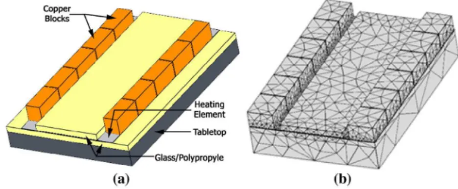
Figure 3 (a) 3-D geometry used in FEM of the weld process. (b) Triangular mesh for inite element analysis of all components
of the heating element. Even though the equation applies to a current through an individual wire and not a meshed element, it does nonetheless approximate the resistivity quite well, with the current and power generation in the model closely resem-bling that of the experiments.
Electrostatic boundary conditions
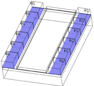
Performing a weld with the CRW requires the movement of the electrodes across the copper blocks. In the model, that trans-lates to shifting the voltage from one pair of copper blocks to the next. To accomplish this, a modiied step function that is C2
continuous was used to apply the voltage, and then remove it. All the remaining boundaries were set to be electrically insulated, that is no current in or out of the boundary. The voltage was applied at the interface between the copper block and the heating element rather than atop the copper blocks to ensure that the current lowed across the width of the heating element instead across adjacent copper blocks. The boundary conditions are indicated with line drawing in Fig. 4, where each voltage (V) has a corresponding ground (G).
Heat transfer modeling
Heat transfer lawsFourier’s law of conduction states that the heat lux and tem-perature gradient are directly proportional to each other.24 In
diferential form the 3-D conduction equation becomes
where ρ is the material density, Cp is the speciic heat capacity
at constant pressure, k is the thermal conductivity, T is absolute temperature and Q is the rate of heat generation.
Both convective and radiation heat transfer boundary conditions are incorporated in the model. The steady-state form of Newton’s Law of Cooling describes a body’s loss of heat transfer occurring between a body and its surrounding ambient luid.24 Natural convection is then described as
(4) 𝜌Cp𝜕T 𝜕t −k ( 𝜕2T 𝜕x2 + 𝜕2T 𝜕y2 + 𝜕2T 𝜕z2 )
Model geometry
The 3-D model geometry shown in Fig. 3(a) has an overall length of 76.2 mm, and a width of 50.8 mm. The heating ele-ment, modeled as a full block, is a 304 stainless steel mesh with a plain weave of 78.74 × 78.74 per square cm (200 × 200 wires per square inch) and a wire diameter of 0.05334 mm (0.0021 inch). Twill glass-iber embedded in a polypropylene (PP) matrix with a iber volume fraction of 34% is used as the laminate with an overall thickness of 2.25 mm. Matching the laminate, the neat resin ilm comprises a 0.16 mm thick PP layer on either side of the heating element. The copper blocks are each 1.2192 cm (0.48 inch) wide with 5.08 mm (0.02 inch) gap between adjacent blocks. They are ofset from the com-posite laminate by 1.0 mm. The gray component in the igure is the 9.525 mm (0.375 inch) electrically insulated thick tabletop that was used to weld the coupon on during experiments.
COMSOL’s auto generated 3-D mesh for inite element anal-ysis did not allow for convergence when solving. Instead, the auto mesh feature was used to give an initial mesh and then manually modiied and run. This was accomplished several times until the solver converged when solving. The mesh con-sisted of 44,471 tetrahedral elements, with 17,010 of those ele-ments contained in the heating element. The heating element is the source of the heat generation in the model, and was thus given a much iner mesh to ensure a smooth solution, a much coarser depiction of which is presented in Fig. 3(b).
Electrostatic modeling
Traditionally the electrostatic modelling assumes power sup-plied to the heating element with a stationary heat source. The result would be then a uniform heat distribution along the heating element. Lambing9 observed that uneven heating
can occur in the heating element depending on the size. On the contrary, modeling the heat source as an electric potential, using fundamental electrostatic equations, does not assume the heat is uniformly distributed. Rather, the current density is calculated at every node in the mesh, and thus the resistive heating that occurs is also calculated by means of the resist-ance. The signiicance of this is that the heating is nonuniform, and the amount of current which exists outside of the weld zone, described as current leakage is known.
Ohm’s law describes the relationship between the current density at a certain spatial point and the electric ield or elec-trostatic potential at that point. The diferential form of this equation for an isotropic material is
where σ is the electrical conductivity of the material, and ∇⃗
is the divergence of the applied voltage V or the electrostatic potential at the point of interest.
Electrical conductivity of the heating element
To model this, the electrical conductivity (σ) of the heating element is determined using Eq. (3)
where, the resistance R is determined experimentally by relat-ing a known ixed applied voltage across it and measurrelat-ing the corresponding current, A is cross-sectional area, and l is length (2) ⃗ ∇(� ⃗∇V ) = 0 (3) 𝜎= l R⋅ A
Figure 4 Electrostatic boundary conditions in the FEM indicated with the line drawing with applied voltage (V) and the corresponding ground (G) across each weld section
Zammara et al. Three-dimensional transient model
Advanced Manufacturing: Polymer & Composites Science 2017 VOL. 3 NO. 1 36
physics together. The result is a heat source that is nonuni-formly spread throughout the heating element.
With the exception of the bottom surface in Fig. 3(a), which was set to have a constant temperature of 25 °C, all boundaries were set to have both convection and radiation conditions. The value of the heat transfer coeicient, h̄, was set to be 5 W/ (m2 K), a value commonly used in several other studies.16,28–30 In
accordance with the same studies, gray bodies radiating with the atmosphere with an emissivity of 0.95 were assumed for all boundaries. The atmospheric temperature was set to 25 °C. The initial temperature for all boundaries was set according to the pre-weld thermocouple readings during experiments for each particular voltage.
Experimental setup
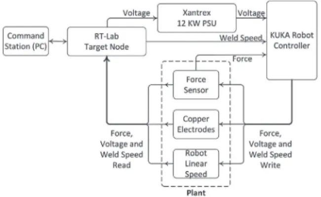
To validate both the electrostatics and heat transfer aspect of the COMSOL model, experiments were run using a KUKA KR 210 robot with the end-efector attached to perform the weld. A Xantec 12 kW power supply was operated in voltage control mode and with constant voltages set in the robot program as an output. The voltage and current signals were measured using RT-Lab, a QNX node that was conigured for data acqui-sition. Figure 5 shows the block diagram for the experimental setup.
In addition to the welding setup as in Fig. 5, data acquisi-tion pertaining to the validaacquisi-tion of heat transfer required plac-ing thermocouples at the weld interface. Shown in Fig. 6(a) is a top view of the experimental setup for the workpiece. The three circles indicate the locations at which the actual tem-perature was measured. A National Instruments (NI) SC-2345 K-type (Al–Cr) thermocouple acquisition system was used to measure the temperatures at those three locations that occur on the heating element at 4, 5, and 6 V. All experiments were run at a weld speed of 1.69 mm/s (4 inch/min). To ensure a strong contact, a pressure of 1.5 MPa was maintained by the pneumatic system and compaction wheel (Fig. 2) on the cop-per blocks. The thermocouples were insulated with Kapton polyimide ilm to prevent the electrical weld current from corrupting the temperature readings as was used by Talbot et al.29 The Kapton was 0.12 mm thick, which is a signiicant
inclusion in the weld stack considering that the PP ilm is 0.16 mm thick. To account for this inclusion all temperature data extracted from the model were taken 0.12 mm above the heating element.
where Qc is the convective heat transfer rate, h̄ is the over-all heat transfer coeicient, Tb is the body temperature, and T∞ is the ambient temperature. Radiation heat transfer was deined using the Stefan–Boltzmann law for nonblack body [24].
Radiation between a body and the atmosphere is described as
where Qr is the radiation heat transfer, ε is the emissivity, σs is the Stefan–Boltzmann constant deined as 5.67 × 10⁻⁸ W/
(m2K4), and T
∞ is the ambient temperature. Material properties
The physical properties are required for use in COMSOL to solve the diferential equations. Without proper values for the physical properties, the model would not yield accurate results. The values for thermal conductivity and density for the 304 stainless steel heating element, PP resin ilm, and the glass/PP laminate were obtained from Harvey25 and Uhlmann
et al.26 with anisotropic thermal conductivity assumed for the
glass/PP. Fujino and Honda27 was consulted for the speciic
heat capacity of the PP resin ilm as a function of temperature.
Heat transfer boundary conditions
When solving Eq. (2), COMSOL also calculates the resistive heating that results from calculated current. This resistive heating term is the term Q in Eq. (4) when solving the heat equation. The approach establishes a link between the elec-trostatics and the heat transfer, essentially coupling the two
(5)
Qc=h(T̄ b−T∞)
(6)
Qr= 𝜖𝜎s(T4b−T∞4)
Figure 5 Block diagram of the experimental setup used for validating the electrostatics of the COMSOL model
Figure 6 Dark circles showing the location of the thermocouples in the weld stack, placed directly atop the heating element: (a) top view and (b) side view
assumption is made that the resistance is the same across each weld section (Fig. 6(a)), then as the electrode is in transition between copper blocks and hence in contact with both of them, the efective resistance is half of the original resistance, R. This lower efective resistance causes the rise in current.
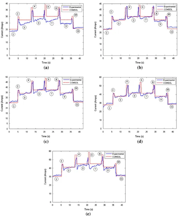
The 11 key points marked with circled numbers on Fig.
7(a)–(e) are locations in which a change in the current occurred in the model. The current generated during the welding pro-cess is of cyclical pattern involving a stable current followed by a brief spike. Table 1 displays the percentage error between the model and experimental measurements for these 11 key points shown on Fig. 7(a)–(e). The error between the model and experiments for each key point is typically below 5% with the exception of point six. Point 6 on Fig. 7(a)–(e) depicts the spike in current that occurs during the transition from the third
Simulation and experimental results
Electrostatics validation
The experimental setup described in Section Experimental setup and shown in Fig. 5 were used to obtain the data required to validate the electrostatics of the 3-D model. Shown in Fig. 7(a)–(e) is the comparison between the currents result-ing from the COMSOL model and actual experimentation at ive separate voltages ranging from 4 to 6 V. During the weld process, there exist large and short periodic increases in total current as shown in the results of Fig. 7 marked with the circled even numbers. Each lat portion in Fig. 7 (marked with circled odd numbers) represents the electrodes directly on top of the copper block. As the voltage source transitions from one cop-per block to the next, there is an increase in the current. If the
Figure 7 Comparison between the currents resulting from COMSOL model and actual weld at (a) 4 V, (b) 4.5 V, (c) 5 V (d) 5.5 V and (e) 6 V
Zammara et al. Three-dimensional transient model
Advanced Manufacturing: Polymer & Composites Science 2017 VOL. 3 NO. 1 38
to low and distribute along the length of the weld coupon. The total current is lower in the irst weld section because it is bounded by the edge of the coupon, and thus an electric ield is created on one side of the heating element. However, as the electrodes move closer to the middle of the weld, Fig. 8(b) and (c), an electric ield is created on the heating element on both sides of the source voltage. This then creates a distribution of current on either side of the source voltage, resulting in a larger total current.
Figure 9 depicts the model’s prediction of the distribution of resistive heating along the vertical line in Fig. 8(c) while welding from the third to the fourth copper block section at 6 V. The vertical lines in Fig. 9 denote the width and location of the third and fourth copper block. The power supplied to the heating element predicted by the model while welding either the third or fourth weld section is 247.0 W. For the third weld section, from Fig. 9, 34.3% of the total power is to fourth sections. The average error across all voltages was
10.42%, which is signiicantly higher than the other points. Also at point 6, the current spike in the experimental value lags that of the model. This was due to a manufacturing defect in the copper blocks. The third copper block was shorter than the rest, and the fourth one was slightly longer. The result was a slight delay during the transition from third to fourth block that ixed itself by the end of the fourth block. In the model, the electrical conductivity of the heating element was not temperature dependent. The higher error could have been attributed to the fact that the resistance did increase slightly as the heating element became hotter.
The total stable current increases from the irst weld sec-tion to the next until it reaches a maximum at the third weld section, or the middle of the weld coupon. This is due to the distribution of the current along the length of the coupon as each section is welded. Figure 8(a) shows the low of the cur-rent, predicted by the model, when welding the irst section. Figure 8(b) and (c) shows the current low for weld sections two and three. During the irst weld section, Fig. 8(a), the voltage is applied across the irst set of copper blocks. The applied voltage creates an electric ield which causes current
Table 1 The percent error between experimental current measurements and the COMSOL model at ive different volt-ages corresponding to locations indicated in Figure 7(a)–(e)
Location % Error At 4.0 V At 4.5 V At 5.0 V At 5.5 V At 6.0 V Average 1 7.31 1.74 4.34 3.42 3.88 4.14 2 8.00 0.72 0.53 1.90 3.38 2.90 3 10.66 1.44 0.16 0.66 1.60 2.90 4 7.50 1.26 4.82 4.97 10.19 5.75 5 7.55 0.17 0.18 1.03 3.70 2.53 6 15.19 6.31 8.56 10.10 11.93 10.42 7 9.95 1.05 1.22 1.81 5.39 3.88 8 4.31 1.02 1.42 3.57 4.15 2.89 9 12.39 2.73 0.38 1.71 2.80 4.00 10 8.08 2.04 2.08 3.32 4.81 4.07 11 4.37 5.91 3.57 2.27 2.34 3.69
Figure 8 COMSOL model output depicting the direction of the current for the (a) irst, (b) second and (c) third weld section Figure 9 Resistive heating along the vertical line in Figure 8(c) that occurs when welding the 3rd and 4th copper block sections as well as while transitioning between them. The vertical lines show the beginning and the end of each copper block.
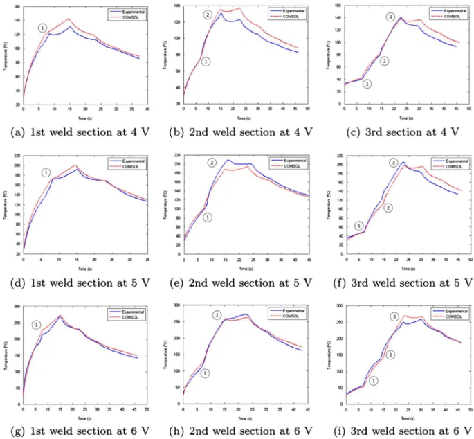
were conducted to validate the COMSOL model. Shown in Fig. 10(a)–(i), are the comparison of the model with the exper-imental measurements. Each weld with ixed parameter set was completed four times, with the data shown representing the median curve of each parameter set. In Fig. 10(a), (d) and (g) the temperature proiles for the irst weld section are pre-sented with each igure signifying the temperature at a particu-lar voltage. Each weld is broken up into several weld sections. A weld section, as shown in Fig. 6(a), is deined as the area of workpieces bounded by the edges of two opposite copper blocks where the voltage is applied. The time the electrodes are supplying power to an individual weld section at 1.69 mm/s (4 inch/min) is 7.2 s. During this time the temperature inside that particular weld section is continuously increasing. Once the electrodes begin to reach the edge of the weld section, they transition to the next weld section. The temperature pro-iles for the second weld section are shown in Fig. 10(b), (e) and (h). Although the electrodes have moved to the next section, there is a residual heating efect that occurs on the irst weld section. This can be seen in Fig. 10(a), (d) and (g) from 7.7 to contained within the boundaries of its copper blocks. At 6 V,
the current passing through the third copper block section is therefore approximately 14.1 A. While the electrodes are transitioning between the third and fourth blocks, the total power supplied to the entire heating element is 321.8 W, as predicted by the model. Of this, 54.4% of the total power is contained between the third and fourth blocks. The resulting current passing through the two copper block sections simul-taneously is then 29.1 A. Figure 9 shows that the distribution of the power is symmetric across the two copper blocks while transitioning between blocks. This results in an individual cur-rent of approximately 14.55 A across each copper section. This result then shows that although the power does dramatically increase while transitioning between two copper blocks, the actual current passing through each block does not change.
Heat transfer validation
A series of experiments, using the experimental setup described in Section Experimental setup and Figs. 5 and 6,
Figure 10 Temperature comparison between simulation and experiments at an weld speed of 1.69 mm/s (4 inch/min). (a) 1st weld section at 4 V, (b) 2nd weld section at 4 V, (c) 3rd section at 4 V, (d) 1st weld section at 5 V, (e) 2nd weld section at 5 V, (f) 3rd weld section at 5 V, (g) 1st weld section at 6 V, (h) 2nd weld section at 6 V and 0(i) 3rd weld section at 6 V
Zammara et al. Three-dimensional transient model
Advanced Manufacturing: Polymer & Composites Science 2017 VOL. 3 NO. 1 40
steel mesh on either side of it allowing the heat to disperse along the mesh adjacent to both sides of the weld section. It is worth noting that at 4 V secondary heating only occurs signiicantly in the irst weld section.
Table 2 presents the error percentages of the transition points that are labeled on Fig. 10 for all three voltage settings. All the errors are typically below 8%, while all are less than 15%. There is some slight uncertainty that exists due to the possible motion of the thermocouple. Once the weld interface becomes completely molten, it is much easier for the thermo-couple to shift slightly. Here, we have done a simple sensitivity test. Using the COMSOL model, in addition to the midpoint of the section, the temperature is measured at 2 mm ahead (in terms of welding direction) of the midpoint. With 4 V applied to the irst section, Fig. 11(a) shows the preheat temperature proile directly on the heating element across the second weld section. The temperature diference at the midpoint of sec-tion two and 2 mm ahead of secsec-tion two is 11%. Figure 11(b) shows the irst section with 4 V applied to it. The variation in temperature from the midpoint to 2 mm ahead of it (in terms of welding direction) is only 4.5%. In this case, the section has a voltage applied directly to it, and so the application of power causes less variation in temperature in the area close to the midpoint. For the preheat case, the heating is a residual efect, and so the further away from the heat source the thermocou-ple gets, the more signiicant the variations are.
Discussions and concluding remarks
A 3-D model was created for the CRW process of thermoplastic materials. The model distinctly and elaborately incorporates both the physics of electrostatics as well as the heat transfer 14.4 s. This occurs because of two reasons. Firstly, the
electri-cal ield resulting from the applied voltage causes current to low in those adjacent sections, as was discussed in Section Experimental setup. Secondly, when the temperature rises in the second section, heat is transferred to the adjacent section.
This same phenomenon causes a noticeable increase in the temperature of the section ahead of the one being welded. Since the weld section has yet to be welded, this is referred to as “pre-heating”. The preheat temperature is then deined as the temperature in the weld section at the instant the voltage is tran-sitioned from one weld section to the next. Each temperature plot is labeled with numbers indicating the key points that were used to compare with the COMSOL model. For example, in Fig. 10(i) there are three key points indicating two preheat temperatures and one weld temperature. At 4 V, the preheat temperature on the second section, shown in Fig. 10(b), is approximately 74 °C, which is 43% of the maximum value reached when that section was welded. At 5 V in Fig. 10(e), the preheat temperature for the second section is approximately 98 °C, 53% of its maximum. At 6 V in Fig. 10(h), the preheat temperature is approximately 120 °C, also 53% of its maximum.
The secondary heating that occurs in the irst weld section is more prominent then for the subsequent weld sections. At 6 V, the secondary heating in the irst weld section of the experimental data shown in Fig. 10(g), causes the temperature to rise to 269 °C, an increase of 25.6% over the maximum temperature reached when the voltage was applied on that section. However, the sec-ondary heating in the second weld section causes an increase of only 7.4%. This is mainly due to the fact that the irst weld section is limited by the poor convective boundary condition, efectively trapping the heat inside the weld section prohibiting it from dis-persing. On the other hand, the second weld section has stainless
Table 2 Percentage error between the COMSOL model and thermocouple measurements (TC) for each weld section at 4 V, 5 V and 6 V from Fig. 10(a)–(c), Fig. 10(d)–(f) and Fig. 10(g)–(i), respectively. The transition points are deined on each corresponding igure
Weld section Transition point
At 4 V At 5 V At 6 V
TC Model % Error TC Model % Error TC Model % Error
1st 1st 120.5 124.2 3.07 172.8 170.0 1.62 214.1 228.7 6.80 2nd 1st 79.3 79.5 0.25 103.6 99.5 4.12 120.4 128.8 6.55 2nd 130.8 134.9 3.04 209.2 187.3 11.69 253.0 259.2 2.37 3rd 1st 39.3 42.8 8.91 209.2 187.3 11.69 55.7 52.4 5.92 2nd 77.1 82.1 6.49 127.0 109.2 14.06 141.8 134.4 5.21 3rd 139.8 138 1.29 205.3 197.7 3.69 249.8 269.1 7.76
Figure 11 Temperature of the heating element across the (a) 2nd and (b) 1st weld sections, respectively, while the irst section has 4 V applied across it.
8. S. H. McKnight, S. T. Holmes, J. W. Gillespie, C. L. Lambing and J. M. Marinelli: ‘Scaling issues in resistance-welded thermoplastic composite joints’, Adv. Polym. Technol., 1997, 16, (4), 279–295.
9. C. L. T. Lambing, R. C. Don, S. M. Andersen, S. T. Holmes, B. S. Leach, andJ. W. Gillespie Jr: ‘Design and manufacture of an automated resistance welder for thermoplastic composites’, in ‘ANTEC’91’, Vol. 91, 2527–2531;
1991.
10. K. D. Tackitt and J. W. Gillespie: ‘Through transmission ultrasonics for process monitoring of thermoplastic fusion bonding’, Proceedings of the 11th technical conference of the American Society for Composites (ACS), Atlanta, GA, October 1996, 1996, 812–821.
11. S. M. Andersen, R. Don, J. Gillespie, S. Holmes, C. L. Lambing and S. Leach: ‘Apparatus and method for resistance welding’, US Patent 5,225,025, 6 July 1993.
12. A. Yousefpour and M.-A. Octeau: ‘Resistance welding of thermoplastics’, US Patent App. 11/887,847, 8 April 2005.
13. I. A. Zammar, I. Mantegh, M. S. Huq, A. Yousefpour and M. Ahmadi: ‘Intelligent thermal control of resistance welding of iberglass laminates for automated manufacturing’, IEEE/ASME Trans. Mechatron.,
2015, 20, (3), 1069–1078.
14. C. Ageorges, L. Ye, Y.-W. Mai and M. Hou: ‘Characteristics of resistance welding of lap shear coupons. Part I: heat transfer’, Compos. Part A: Appl. Sci. Manufac., 1998, 29, (8), 899–909.
15. T. B. Jakobsen, R. C. Don and J. W. Gillespie: ‘Two-dimensional thermal analysis of resistance welded thermoplastic composites’, Polym. Eng. Sci., 1989, 29, (23), 1722–1729.
16. S. T. Holmes and J. W. Gillespie: ‘Thermal analysis for resistance welding of large-scale thermoplastic composite joints’, J. Reinf. Plast. Compos.,
1993, 12, (6), 723–736.
17. X. Xiao, S. Hoa and K. Street: ‘Processing and modelling of resistance welding of APC-2 composite’, J. Compos. Mater., 1992, 26, (7), 1031–1049. 18. R. Don, L. Bastien, T. Jakobsen and J. Gillespie: ‘Fusion bonding of
thermoplastic composites by resistance heating’, SAMPE J., Jan.–Feb.
1990, 26, (1), 59–66.
19. R. Carbone and A. Langella: ‘Numerical modeling of resistance welding process in joining of thermoplastic composite materials using comsol multiphysics’, COMSOL Conference, Milan, 2009.
20. A. Mafezzoli, J. Kenny and L. Nicolais: ‘Modelling of thermal and crystallization behavior of the processing of thermoplastic matrix composites’. Materials and Processing DH Move into the 90’s, 1989a, 133–143.
21. A. Mafezzoli, J. Kenny and L. Nicolais: ‘Welding of peek/carbon iber composite laminates’, SAMPE J., 1989b, 25, (1), 35–40.
22. L. Bastien and J. Gillespie: ‘A non-isothermal healing model for strength and toughness of fusion bonded joints of amorphous thermoplastics’, Polym. Eng. Sci., 1991, 31, (24), 1720–1730.
23. A. Smiley, A. Halbritter, F. Cogswell and P. Meakin: ‘Dual polymer bonding of thermoplastic composite structures’, Polym. Eng. Sci., 1991,
31, (7), 526–532.
24. J. H. Lienhard: ‘A heat transfer textbook’, 2013, Cambridge, MA, Courier Corporation.
25. P. D. Harvey: ‘Engineering properties of steel’, 1982, Metals Park, OH, American Society for Metals.
26. E. Uhlmann, G. Spur, H. Hocheng, S. Liebelt and C. Pan: ‘The extent of laser-induced thermal damage of UD and crossply composite laminates’, Int. J. Mach. Tools Manuf, 1999, 39, (4), 639–650.
27. J. Fujino and T. Honda: ‘An investigation on measurement accuracy of speciic heat capacity using a heat lux diferential scanning calorimeter (in the case of polyethylene, acrylic resin and plastic composite)’, Proc. ‘45th Japanese Conf. Calorimetry and Thermal Analysis’, September 28–30, 2009, Tokyo, Japan, Tokyo Metropolitan University.
28. D. Stavrov, G. F. Nino and H. E. Bersee: ‘Process optimization for resistance welding of thermoplastic composites’, In 47th AIAA/ASME/ASCE/ AHS/ASC Structures, Structural Dynamics, and Materials Conference 14th AIAA/ASME/AHS Adaptive Structures Conference 7th (p. 2246), Newport, RI, May 2006.
29. E. Talbot, A. Yousefpour, P. Hubert and M. Hojjati. ‘Thermal behavior during thermoplastic composites resistance welding’, Aannual Technical Conference (ANTEC) of the Society of Plastics Engineers, Boston, MA, 2005.
30. S. Tan, G. Zak, P. Bates and J. Mah: ‘Resistance welding of glass-iber reinforced pp modeling and experiments’, Proc. ANTEC 2006, Charlotte, NC, May 2006, Society of Plastics Engineers, 2236–2240.
that are present in the process. The electrostatics model cor-related with experimental measurements with less than 5% error. The trend in the current while welding was reproduced accurately with the model showing peaks in current that existed in the experiments. On the heat transfer side of the model, the key points that were compared had typically less than 10% error between the model and the experiments. The model also reproduced the preheating phenomenon that was observed experimentally.
One of the major items gained from the model was the knowledge of how the resistive heating is distributed through-out the heating element as the rollers move along the work-pieces. In the static welding case a typical current of 12 A at 4 V would exist, where as in the continuous case the current would be upwards of 20 A.
In the actual feedback temperature control scenario of the full-scale CRW, it is not feasible to measure the actual online weld temperature using thermocouples. This is because it is either sealed in the weld interface, or blocked by the end-ef-fector’s compaction track. The model has been successfully used to derive linear state-space observer that would estimate the temperature at the weld interface online.13 Due to the
dis-crete nature of the CRW process, there is no continuous accu-mulation of heat. The preheat temperature at a given voltage and speed is the same for all weld sections away from the boundary of the coupon. This was advantageous because it allowed the use of a linear observer to estimate the online weld temperature, and assume a constant initial temperature for all weld sections. It was shown that this is indeed the case, and that the preheat temperature at 6 V was only a function of the prior two weld sections.
Disclosure statement
No potential conlict of interest was reported by the authors.
Funding
This work was supported by the Canadian Network for Research and Innovation in Machining Technology, Natural Sciences and Engineering Research Council of Canada (NSERC); National Research Council Canada (NRC).
References
1. J. George, M. Sreekala and S. Thomas: ‘A review on interface modiication and characterization of natural iber reinforced plastic composites’, Polym. Eng. Sci., 2001, 41, (9), 1471–1485.
2. A. Yousefpour, M. Hojjati and J.-P. Immarigeon: ‘Fusion bonding/welding of thermoplastic composites’, J. Thermoplast. Compos. Mater., 2004, 17, (4), 303–341.
3. S. R. Reid and G. Zhou, eds: ‘Impact behaviour of ibre-reinforced composite materials and structures’, 2000, Cambridge, UK, CRC Press. 4. X. Zhang, C. Lu and M. Liang: ‘Preparation of thermoplastic vulcanizates based on waste crosslinked polyethylene and ground tire rubber through dynamic vulcanization’, J. Appl. Polym. Sci., 2011, 122, (3), 2110–2120.
5. A. Benatar and T. G. Gutowski: ‘Method for fusion bonding thermoplastic composites’, SAMPE Q.,(United States) 1986, 18, (1), 35–45.
6. S. M. Todd: ‘Joining thermoplastic composites’, Proceedings of the 22nd international SAMPE technical conference, 1990, 22, 383–392. 7. R. A. Grimm: ‘Welding processes for plastics’, Adv. Mater. Processes, 1995,
147, (3), 27–30.