Feature Preserving Mesh Generation from 3D Point Clouds

HAL Id: inria-00497632

https://hal.inria.fr/inria-00497632

Submitted on 5 Jul 2010

HAL is a multi-disciplinary open access

archive for the deposit and dissemination of

sci-entific research documents, whether they are

pub-lished or not. The documents may come from

teaching and research institutions in France or

L’archive ouverte pluridisciplinaire HAL, est

destinée au dépôt et à la diffusion de documents

scientifiques de niveau recherche, publiés ou non,

émanant des établissements d’enseignement et de

recherche français ou étrangers, des laboratoires

Feature Preserving Mesh Generation from 3D Point

Clouds

Nader Salman, Mariette Yvinec, Quentin Mérigot

To cite this version:

Nader Salman, Mariette Yvinec, Quentin Mérigot. Feature Preserving Mesh Generation from 3D

Point Clouds. Computer Graphics Forum, Jul 2010, Lyon, France. pp.1623-1632. �inria-00497632�

Olga Sorkine and Bruno Lévy (Guest Editors)

Feature Preserving Mesh Generation from 3D Point Clouds

1_{INRIA Sophia-Antipolis}

Abstract

We address the problem of generating quality surface triangle meshes from 3D point clouds sampled on piecewise smooth surfaces. Using a feature detection process based on the covariance matrices of Voronoi cells, we first ex-tract from the point cloud a set of sharp features. Our algorithm also runs on the input point cloud a reconstruction process, such as Poisson reconstruction, providing an implicit surface. A feature preserving variant of a Delaunay refinement process is then used to generate a mesh approximating the implicit surface and containing a faithful representation of the extracted sharp edges. Such a mesh provides an enhanced trade-off between accuracy and mesh complexity. The whole process is robust to noise and made versatile through a small set of parameters which govern the mesh sizing, approximation error and shape of the elements. We demonstrate the effectiveness of our method on a variety of models including laser scanned datasets ranging from indoor to outdoor scenes.

Categories and Subject Descriptors(according to ACM CCS): [Computational Geometry and Object Modeling] [I.3.5]: Curve, surface, solid, and object representations—

1 Introduction

Surface reconstruction consists in inferring the shape of an object from a 3D point cloud sampled on the surface. The problem of automatic surface reconstruction from point sam-ples has received considerable amount of efforts in the past twenty years. Surface reconstruction problems occurs in dif-ferent flavors according to the quality of the data which are more or less entangled with noise, and the properties of the reconstructed object whose surface can be smooth or struc-tured with sharp features. Moreover, an implicit description of the reconstructed object is enough for some applications, whereas some other require a data structure more amenable to further processing, like a mesh.

In this paper, we focus on the case where the sampled surface is piecewise smooth and the output sought after is a high quality triangle mesh approximating the surface. Our goal is to generate from the input point cloud a mesh including a faithful representation of sharp edges, thus improving the trade-off between the accuracy and the size off the mesh. We propose for that an algorithm which experimentally proves to be fairly robust to noise.

1.1 Related work

Reconstruction and quality surface mesh generation are of-ten tackled separately in the literature. We first review the approaches dealing with the problem of robust reconstruc-tion of piecewise smooth surfaces, before reviewing the

ap-proaches that combine reconstruction and quality surface mesh generation.

1.1.1 Towards piecewise smooth reconstructions.

In the quest to achieve both noise robustness and recovery of sharp features, we can identify an evolution of approaches ranging from smooth to sharp.

Smooth surfaces.As noise and sparseness are common in laser scanner datasets, we have seen in recent years a vari-ety of approaches for robust reconstruction of smooth sur-faces. A popular approach consists of searching an implicit function whose zero level set fits the input data points. The searched implicit functions can take different forms, being for instance approximated signed distance functions to the inferred surface [OBA05,GG07] or approximated indicator functions of the inferred solid [KBH06]. Implicit functions methods often provide spectacular robustness to noise. How-ever most of them assume that the data points come with ori-ented normals and are sampled from a smooth surface. The latter assumption leads to erroneous surface reconstruction at locations where the smoothness assumption is not met. An intermediate step toward handling sharp features con-sists of using locally adapted anisotropic basis functions when computing the implicit function [DTS01]. Adamson and Alexa [AA06] perform piecewise polynomial approx-imation through anisotropic moving least-squares (MLS). More recently, Oztireli et al. [OGG] used a kernel

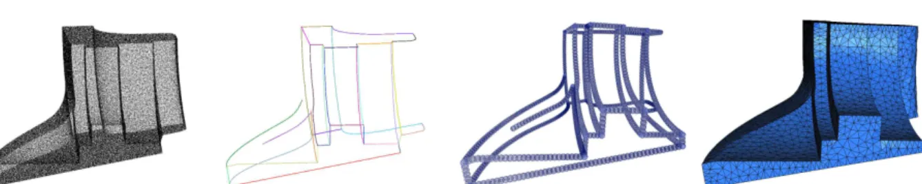
regres-Figure 1: Overview of the method at a glance. From left to right: given a point cloud sampled on a piecewise smooth surface; detect the

potential sharp edges points, cluster them with respect to the underlying sharp features direction, and extract explicit polylines for each cluster; sample protecting balls on the extracted polylines; combine extracted polylines to implicit surface reconstruction through feature preserving mesh generation to output a 3D mesh where the sharp edges are explicitly tesselated and appear as a subset of the triangle edges.

sion technique to extend the MLS reconstruction to surfaces with sharp features.

While satisfactory for some applications (e.g., visualization as opposed to mesh generation), these approaches generate surfaces which are more accurate around sharp features but are still smooth. In addition, boosting the anisotropy of a function is a dangerous game when simultaneously target-ing robustness to noise, as such a strategy may amplify noise instead of the true features (features and noise are ambigu-ous as both are high frequency). Furthermore, a purely local distinction between smooth parts and sharp edges is likely to yield fragmented edges while a global feature extraction approach can favor long edges in order to recover the true structure.

Handling sharp features.This brings out another thread of work aimed at extracting long sharp features. Pauly et al. [PKG03] use a multi-scale approach to decide if a point is on a feature, and construct a minimum-spanning tree to recover the feature graph. Daniels et al. [DHOS07] extract feature-curves using a method based on a robust MLS projection op-erator which locally projects points onto the sharp edges, and grow a set of polylines through the projected points. Jenke et al. [JWSA08] extract the feature lines by robustly fitting local surface patches and by computing the intersection of close patches with dissimilar normals. Both methods show satisfactory results even for defect-laden point sets. More re-cently, Merigot et al [MOG09] proposed a robust estimation of curvature tensors based on a covariance measure defined from the data points Voronoi cells. Their method provides theoretical guarantees on robustness under bad sampling and noise conditions.

One way to make a local, binary distinction between smooth parts and sharp features consists of performing a local clus-tering of the inferred normals to the surface [OBA∗_{03]. If}

this process reveals more than one cluster, the algorithm does not fit just one low-degree implicit function, but as many quadrics as the number of clusters. This leads to faithful lo-cal reconstruction of a sharp edge as the intersection of two implicit primitives in the case of two clusters. A corner is reconstructed as the intersection of three or more primitives.

Note in passing that the method misses tips (sharp point that are not incident to any sharp crease), cusps and darts. In order to achieve improved robustness, Fleishman et al. [FCOS05] segment neighborhoods of points by growing re-gions belonging to the same part of the surface. Robustness is obtained by using a forward search technique which finds reference planes corresponding to each region. While consti-tuting an important progress, the method requires very dense point clouds, and is rather expensive. Also, potential instabil-ities in the classification can create fragmented surface parts. Targeting even higher robustness, Lipman et al. [LCOL07] enrich the MLS projection framework with sharp edges by defining a singularity indicator field based on the error of the MLS approximation. However, they choose to restrict their approach to a single singularity within each influence radius, which significantly limits the type of feature points that can be handled.

1.1.2 Coupling reconstruction and mesh generation.

One popular approach that couples reconstruction and mesh generation is the extended marching cubes introduced by Kobbelt et al. [KBSS01]. The input is assumed to be a dis-cretized signed distance function enriched with oriented nor-mals, the latter being used to decide whether or not a voxel contains a sharp feature. If a voxel is classified as contain-ing a feature, some additional vertices are constructed within the voxel and placed at intersections between the planes de-fined by the vertices and their affiliated normals. This ap-proach works robustly and efficiently by truly coupling fea-ture extraction and mesh generation. Nevertheless, it relies on the marching cubes process which is well known to pro-duce rather poor quality surface meshes.

Two approaches which are able to generate quality surfaces while preserving the features [DHOS07,JWSA08] proceed sequentially by first extracting a set of features, then us-ing the advancus-ing front method proposed by Schreiner et al. [SSFS06]. The latter produces quality isotropic meshes from different inputs including MLS representations, and can con-trol the density of the mesh by pre-computing a guidance field. The algorithm uses time-consuming pre-processing of the point cloud in order to construct a guidance field, as well as a final post-processing using MLS projections.

A relevant alternative to the marching cubes and advanc-ing front strategies is the Delaunay refinement paradigm [BO05]. In this method the surface mesh is intersection free by construction as filtered out of a 3D Delaunay triangula-tion. A number of additional guarantees are also provided after termination of the refinement process, such as a good shape of elements, a faithful approximation of geometry and normals, and a low complexity of the mesh. More interest-ingly in our context, Delaunay refinement is able to couple reconstruction and mesh generation. At the intuitive level, the refinement procedure is combined with a sensing al-gorithm probing an implicit surface defined from the data points. The probing is performed along Voronoi edges of sampling points which are not only longer than the short edges of the marching cubes but also data-dependent as they become more and more orthogonal to the sensed surface as the refinement process goes along.

However, in [BO05] sharp features are not explicitly han-dled, hence they are not accurately represented in the output mesh. One way to circumvent this drawback is to extract the feature lines and to constrain the Delaunay refinement to preserve them. However, it is well known that the presence of constrained edges where meeting surface patches form small angles, endangers the termination of the Delaunay re-finement [She00]. Recently Cheng et al. [CDR07,CDL07] propose to deal with this problem using the method of pro-tecting balls set up around sharp features.

1.2 Contributions

In this paper, we argue that some modifications of the im-plicit smooth surface reconstruction algorithms can produce results with accuracy on par with the best current piecewise smooth reconstruction methods. Given a 3D point cloud sampled on a piecewise smooth surface, our algorithm con-sists of two steps. In the first step, we extract from the in-put 3D point cloud a set of polylines approximating the sharp edges of the object. This feature extraction is based on the robust feature estimation framework of Merigot et al. [MOG09]. In parallel, our algorithm runs on the data points a reconstruction process, providing an implicit surface, i.e. an implicit function whose zero level sets approximates the data points. The second step of our algorithm generates a mesh approximating the implicit surface while including a faithful representation of the extracted sharp edges. This step runs a feature preserving version of the Delaunay refinement meshing algorithm, based on the meshing algorithm of Bois-sonnat and Oudot [BO05] and using the mechanism of pro-tecting balls introduced by Cheng et al. [CDR07,CDL07]. An overview of the method is illustrated in Figure1. The technical tools used in this algorithm are directly in-spired by recent work [MOG09,CDL07]. However, they have not been used previously in this combination, and we argue that it is this particular synthesis of existing ideas which is the key of its success.

The main benefits of our algorithm are: Accuracy. The

method provides a meshed representation of a point sam-pled object with an enhanced trade-off between accuracy and mesh size. Robustness. The method is robust to noise and stable under sparse sampling. Flexibility. The method offers considerable flexibility as it can be tuned with respect to the scale and the targeted size of the mesh.

2 Feature extraction

2.1 Feature detection

A point on a piecewise-smooth surface, is called a (sharp) feature point, if the surface has no tangent plane at this point. The locus of feature points on a piecewise-smooth surface has the structure of a graph.

We are given a point cloud P sampling a piecewise-smooth surface S. In order to allow the mesh generation algorithm to faithfully reproduce the sharp features of S, we need to extract from the input point cloud an approximation of the feature graph of S. Our first goal is to identify the data points that are close to sharp edges. To this aim, we use the method of Merigot et al. [MOG09] based on an analysis of the shape of Voronoi cells through their covariance matrices.

Recall that the covariance matrix of a bounded domain E of R3with respect to a base point p is defined by cov(E, p) = R

E(x− p)(x− p)

T_{dx. The eigenvectors of this matrix capture}

the principal axes of E while the ratio of the eigenvalues gives information on the anisotropy of E.

The Voronoi diagram of the sampling P is the cellular de-composition of the space, where each sample p ∈ P has a cell, V (p), that is the locus of points closer to p than to any other sample in P :

V(p) = {x ∈ Rd: ∀q ∈ P,kx − pk ≤ kx − qk} By construction, the shape of Voronoi cells depends on the whole set of data, and some cells are unbounded. In order to get more local information, [MOG09] introduce an offset parameter R and consider for each data point p of P, the co-variance matrix, M(p,R), of the intersection of the Voronoi cell V (p) with a ball, B(p,R), of radius R centered at p:

M(p, R) = cov (V (p) ∩ B(p, R), p)

The principal drawbacks of Voronoi-based methods is their high sensitivity to noise. To alleviate the effect of noise, [MOG09] smoothes the information contained in the co-variance matrices using convolution. The method computes for each point p the convolved Voronoi covariance matrix (CVCM), Mc_{(p, R, r), by summing the covariance matrices}

of all points q of P at a distance less than r to x:

Mc(p, R, r) =

_∑

q∈B(p,r) M(q, R)

The crucial remark is that sample points lying on smooth surfaces, called

smooth points, have a pencil shaped Voronoi cell; hence their CVCM has two “small” eigenvalues and a larger

one, with the eigenvector corresponding to the large eigen-value directed along the surface normal. Sample points that are close to sharp edges, called edge points, have rather flat Voronoi cells; therefore there CVCM has a single “small” eigenvalue and two larger ones, and the eigenvector corre-sponding to the small eigenvalue is directed along the edge. Sample points close to feature graph nodes, called corner

points, tend to have cone-shaped Voronoi cells thus all three

eigenvalues have comparable values.

Based on those observations, the algorithm we use to de-tect feature points (edge and corner points) is the following. We compute the CVCM, Mc_{(p, R, r), of each point p ∈ P,}

and sort the eigenvalues of this matrix by decreasing order λ₀(p) ≥ λ₁(p) ≥ λ₂(p). If the ratio λ₀(p)/λ₁(p), is greater than a threshold t1, p is a smooth point. Else, if the ratio

between λ₁(p)/λ₂(p), is greater than a threshold t₂, p is an edge point. Else, point p is a corner point. We gather, in a set F, the pairs (p,e2(p)), where p is a point classified as

an edge point and e2(p) is the eigenvector of its CVCM

corresponding to the smallest eigenvalue λ2(p), which is

supposed to be aligned with the sharp edge direction. Note that we choose not to keep in F, the pairs corresponding to corner points because of the instabilities of the data around these positions. Instead, we will recover corner points as ex-tremities of sharp edges (Section2.3).

Parameters:The method needs four parameters: the offset

ra-dius R, the convolution rara-dius r and both thresholds t1,t2. Parameter

Rshould be chosen smaller than to the external reach of the under-lying surface defined as the smallest distance from a point of the surface to the external medial axis. Parameter r has two different roles: besides smoothing the information, it determines the curva-ture radius under which a curved area is considered as a sharp fea-ture. Consequently, it should be chosen depending on the noise level and on the sizing field of the targeted mesh. In all our experiments, we fixed parameter R to be one tenth of the point cloud bounding sphere radius and r to be a tenth of R, which leads to good results. Moreover, we allow the user to modify t1and t2manually, using an

interactive interface.

Algorithm 1Clustering points in F

Place each point pi∈ F in its own cluster Fi with it’s

potential extremity points Ei= ∅

for allpoints pido

for all pj∈ F such that d(pi, pj) < ρk(pi) do

if pjand piareNOTin the same cluster (Fj6= Fi)

then

Compute angle αi= ∠(e2(pi), pipj)

Compute angle αj= ∠(e2(pj), pipj)

ifαi≤ θ and αj≤ θ then

Merge the clusters Fiand Fj

Merge Eiand Ej

ifαi≤ θ and αj> θ then

Ei← pj

Figure 2: Result of the clustering step on the octa-flower model.

2.2 Feature clustering

In [MOG09], it is proven that the convolved covariance ma-trix is robust to noise, by deriving a bound on the quality of the results as a function of the Hausdorff distance between the point cloud and the sampled surface. However, the re-construction of the sharp feature graph is left unaddressed in this work. Here, we need to approximate the sharp edges with polygonal lines. In their work [DHOS07] presented a technique for solving a similar problem. We however pro-ceed differently taking advantage of the edge direction in-formation we get from the CVCM analysis.

Our goal here is to group edge points of F into clusters, where each cluster samples a straight or bending sharp edge. For that, we need a similarity measure that will quantify if two edge points belong to the same sharp edge.

A pair (pi, pj) of edge points is said to be a close pair if

the Euclidean distance d(pi, pj) is less than ρk(pi), where

ρk(pi) =1k

q

∑kl=1|pi− pl|2, the sum running on the k

near-est neighbors to piin F. Two close points pi, pj∈ F belong

to the same cluster if the angles αi= ∠(e2(pi), pipj) and

αj= ∠(e2(pj), pipj) are smaller than a given threshold θ.

This criteria is injected in an union-find algorithm (Algo-rithm1) that partitions points of F into clusters Fi. In

addi-tion, if only one of the angular conditions is satisfied for a close pair (pi, pj), say αi< θ but αj≥ θ, point pjis

clas-sified as an extremity point of cluster Fi and included in

a set Ei of extremity points related to Fi. These extremity

points will be of use to elongate the constructed polylines in Section2.3, facilitating the resolution of the polylines junction recovery problem. Moreover, our implementation prunes clusters consisting of few points (|Fi| ≤ 6) and

unla-bels the potential extremity points associated to them. Parameters:The identification of good clusters relies on an

appropriate selection of parameters θ and k. For big values of θ the detected clusters will be thick, thus it will be hard to sort the clus-tered points, a step we need for recovering the features. For our pur-poses, θ = 15◦_{and k = 20 provided sufficiently thin and}

represen-tative clusters to facilitate the feature recovery procedure (Figure2), without the need to apply the thinning heuristics of [Lee00].

2.3 Feature recovery

In the following our aim is to recover from each cluster, pro-vided by the previous step, a polyline that will best fit the shape of the underlying sharp edge.

For each cluster Fiwe build a polyline Poly(Fi) by

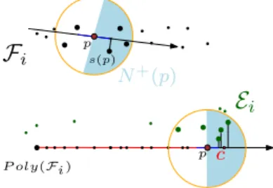
apply-ing iteratively a procedure succ(p) that discovers the suc-cessor of a point p (Figure3top). We start at a random seed point p ∈ Fi. The successor s(p) of p is defined as follows:

we consider the subset N(p) ⊂ Fiof points included in a

ball of radius rp centered at p. All points in N(p) are then

projected onto the line defined by p and the edge direction

e2(p). Points in N(p) can be divided into two subsets by

in-specting the position of their projections relative to p. If p is the starting point, we choose randomly one of the subsets to be N+_{(p). Otherwise, let N}+_{(p) be the subset of points}

whose projections are in the direction opposite to the prede-cessor of p. Then, s(p) is defined as the point in N+_{(p) with}

closest projection to p. The procedure succ(p) is applied it-eratively until an endpoint is reached, i.e. a point for which

N+(p) is empty. The procedure is then restarted from the seed point in the opposite direction.

The polyline Poly(Fi) and the edge directions attached to

its vertices are then smoothed using a standard PCA based smoothing process.

To lengthen the recovered feature polylines Poly(Fi), we use

the detected potential extremity points Ei attached to each

cluster. For each endpoint p ∈ Fi, if Ei is not empty, we

search for neighboring points pj∈ Eisuch as the Euclidean

distance d(p, pj) < rp. All such points are projected onto

the line defined by p and the edge direction e2(p). Then, we

compute the centroid c of the projected points located on the half-line defined by p and not containing the projection of

N(p). Finally, point c is added to the polyline as the suc-cessor of p and attached a direction e2(c) = e2(p). Point c

is considered as the new endpoint of Poly(Fi) (see Figure3

bottom).

Our implementation maintains for each polyline Poly(Fi) a

value corresponding to the polyline length that will be of use in the feature junction recovery step to prevent joining the endpoints of a single short polyline.

Parameters:The recovered polyline result is dependent on the

size of the selected neighborhood. The radius parameter rpshould

be related to the local feature size of the polyline to be recovered. Optimally, one should study the effect of the neighborhood size and propose an optimal neighborhood-size-selection scheme. Prac-tically, we do not have this information, hence we choose rp= ρk(p)

where k = 5.

Junction recovery.In order to build a realistic approxima-tion of the sharp feature graph, we need to construct ap-propriate junctions between the constructed polylines. The task is simplified as we have extended the polylines and thus reduced the search space for potential junctions. Note that

P oly_(Fi)

E

F

Figure 3: Illustration of feature recovery step. Top: procedure

succ(p) that discovers the successor, s(p), of a point p ∈ Fi.

Bot-tom: after smoothing the polyline Poly(Fi), we elongate it at each

endpoint p using the detected extremity points Ei.

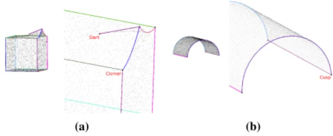
sharp edges joined at vertices of the feature graph are clas-sified as follows: a dart is incident to a single sharp edge; a cusp is incident to two sharp edges forming a sharp angle at the junction; a corner is incident to three or more sharp edges.

A natural solution is to merge in a single vertex, polylines endpoints that are spatially close. We could simply take as position for the merged vertex the barycenter of the merged endpoints. However, to increase the accuracy of the approx-imation of sharp feature junctions we proceed as follows. For each endpoint p of Poly(Fi), we start by constructing

the set J (p) of endpoints that are within a ball B(p,rjunc)

of radius rjunccentered at p. In case there is no endpoint in

J (p) other than p itself, we tag p as a dart and continue. Lj

Lk

pk

pj

qjcqk

Otherwise, |J (p)| ≥ 2 and we compute the junction position as follows. For ev-ery pair of endpoints pj, pk∈ J (p), we

consider the two points qj, qkwhich are

the closest points such that qjbelongs to

the line Lj passing through pj and

di-rected along e2(pj) and qk belongs to the line Lk passing

through pkand directed along e2(pk). The junction point is

computed as the barycenter of the set of closest points, ex-cept that each closest point that is not in the ball B(p,rjunc)

is replaced by the endpoint p in the barycenter computation. Our procedure has the advantage of being easy to imple-ment and is computationally inexpensive since it does not introduce any plane nor surface fitting and intersection com-putations. An example of finding junctions from polylines including three junction cases, darts, cusps and corners is il-lustrated in Figure5. Note that we do not capture tips, i.e. vertices incident to zero sharp edges but are sharp.

Parameters:The radius parameter r_juncshould be chosen large

enough, in order to cover the empty space between polyline end-points. On the other hand, rjuncgenerally shouldn’t be larger than

the length of the shortest polyline – which would lead to both of its endpoints being merged into a single junction. In practice, we found that choosing rjuncto be equal to five times the average spacing of

Figure 4: Left: Feature recovery for the octa-flower model. Right:

Closeup view of the recovered sharp edges and the recovered junc-tion (black dot).

3 Feature preserving mesh generation

Besides extracting sharp edges, our algorithm runs on the data points a reconstruction process, such as Poisson reconstruction [KBH06] or any variant of moving least square [GG07], providing an implicit description of a sur-face approximating the data points. Such an implicit sursur-face is represented as a function (R3→ R) whose zero level set approximates the data points. Our goal in this section is to show how, using a feature preserving variant of a Delau-nay refinement mesh generation algorithm, we obtain a sur-face mesh approximating the implicit sursur-face and including a faithful representation of the sharp edges extracted in the previous section.

3.1 Delaunay refinement surface mesh generation

To generate a mesh approximating the implicit surface, we use the surface meshing algorithm of Boissonnat and Oudot [BO05]. This algorithm is a Delaunay refinement, based on the notion of restricted Delaunay triangulation. Let P be a set of points in R3and S be a surface. The re-stricted Delaunay triangulation, DS(P), is the sub-complex

of the Delaunay triangulation D(P) formed by the faces of D(P) whose dual Voronoi faces intersect S. It has been proven that if P is a “sufficiently dense” sample of S, DS(P) is homeomorph to the surface S and is a good

approximation of S in the Hausdorff sense [ES97,AB99,

BO05].

The meshing algorithm of [BO05] builds on this result. It maintains the restricted Delaunay triangulation DS(P) of a

sampling P of the surface, and refines the sampling P until it is dense enough for the restricted Delaunay triangulation to be a good approximation of the surface. More precisely, the refinement process tracks bad facets in DS(P), i.e. facets

that do not comply to the meshing criteria. Each bad facet is killed out by the insertion of a new vertex at its surface

centerwhich is the point where the Voronoi edge, dual to

the facet, intersects the surface.

Such a Delaunay refinement surface meshing algorithm yields a quality surface mesh, free of self-intersections.

(a) (b)

Figure 5: Junction recovery. (a) a dart and multiple corners are

recovered from the smooth feature model; (b) multiple border cusps are recovered from the half cylinder model

However, since features are not handled explicitly, they are poorly represented in the output mesh (see Figure7middle). Parameters:The parameters of the Delaunay refinement are

the parameters of the criteria defining the bad facets. A facet is bad if either some facet angle is smaller than α, or some facet edge is longer than l or the distance between the center of the facet and the surface is more than d.

3.2 Feature preserving extension

To achieve an accurate representation of the extracted sharp features in the final mesh, we resort to the method of

pro-tecting ballsproposed by Cheng et al. [CDR07] and

exper-imented in [CDL07]. This method performs, before the De-launay refinement, a protecting step in which each sharp fea-ture is covered by a set of protecting balls, such that: ⊲_{protecting balls are centered on sharp features and each} feauture is completely covered by the union of protecting balls centered on it;

⊲any two balls have an empty intersection, except balls with consecutive centers on a given sharp feature that intersect significatively but do not include each other’s center; ⊲any three balls have an empty intersection.

Once the protecting balls have been computed, they are re-garded as weighted points and inserted altogether, as ini-tial vertices, in a weighted Delaunay triangulation. The Delaunay refinement process is then performed using this weighted Delaunay triangulation: at each step, the refine-ment process computes the weighted version of a bad facet surface center. This point is affected a zero weight and in-serted in the weigthed Delaunay triangulation.

Such a weight setting, together with the protecting ball prop-erties, enforces the fact that two protecting ball centers, con-secutive on a sharp feature polyline are guaranteed to remain connected by a restricted Delaunay edge. Furthermore, ow-ing to the fact that no three balls intersect, the refinement process never inserts refinement point in the union of the protecting balls nor probes the surface in this protected re-gion. This ensures the termination of the refinement pro-cess whatever may be the dihedral angle formed by smooth patches incident on a sharp feature.

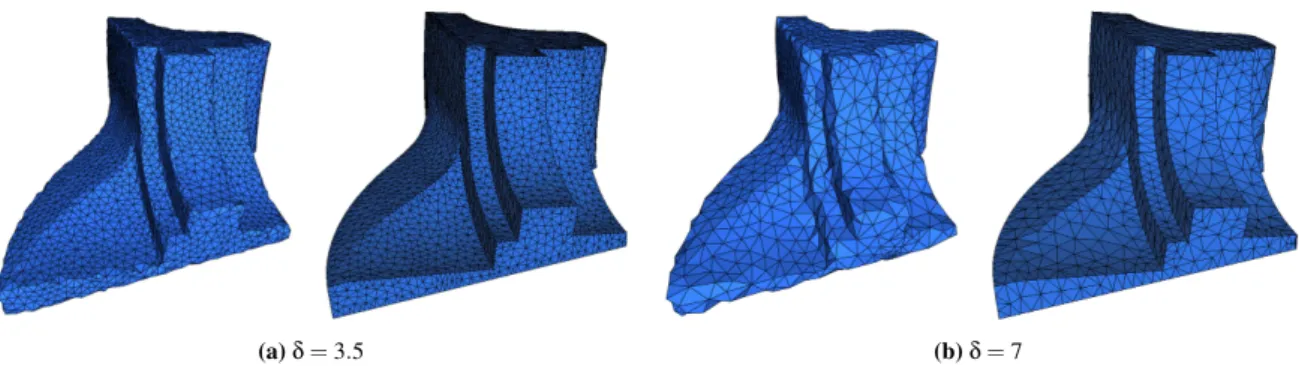
(a)δ = 3.5 (b)δ = 7

Figure 6: Feature preserving mesh generation for the fandisk model. The thresholdδ is used to adjust the size of the protective balls thus

the mesh resolution; for (a) and (b), the meshed Poisson implicit function (PIF) is on the left whereas the meshes generated with our feature preserving extension using PIF are on the right. For both threshold values the extracted polylines and their endpoints are tesselated explicitly.

Protecting balls have a crucial in-fluence on the sizing of the output mesh. On one hand protecting ball centers define the approximation of sharp features in the final mesh, and the sizing parameter l of the

Delau-nay refinement cannot be smaller than the spacing between protecting ball centers. On the other hand, to provide a sur-face mesh with sur-facets incident to the mesh edges approxi-mating a sharp feauture, the refinement process requires that the union of protecting balls covers the gap between the im-plicit surface (orange) and the extracted feature polylines (green, blue).

In practice, to compute the protecting balls, we first keep all endpoint vertices of the detected polylines Poly(Fi) and

then sample points on Poly(Fi) according to some user

de-fined uniform distance d′_{. Then the algorithm tries setting a}

uniform weight wp= 2/3 ∗ d′ on sample points. If the

re-sulting set of balls do not comply with the above rules, it is locally fixed by adding new sample points and reducing ball radii.

Parameters:In our experiments, the mesh generation step

de-pends on a single user-defined parameter δ. Indeed, we use as unit length the quantity avg defined as the mean of the distances from each input data point to each one of its six first nearest neighbors. Then, we fix the protecting ball parameter and Delaunay refinement parameters to: d′_{= δ ∗ avg, α = 25}◦_{, l = 2 ∗ d}′_{, d = 0.6 ∗ d}′_.

4 Experimental results

Our prototype is implemented in C++ using the robust primitives provided by the CGAL library [cga]. We use CGAL 3D triangulation as the core data structure to

com-pute the Voronoi covariance matrices of the input point cloud [MOG09]. The CGALlibrary also provides us with an

imple-mentation of the Poisson reconstruction method [KBH06] to compute an implicit surface from the input point cloud. Lastly CGAL provides an implementation of the Delaunay

refinement surface meshing algorithm of Boissonnat and Oudot [BO05].

A crucial component for reaching good timings is the effi-cient answer to queries for the subset of a point cloud con-tained in a given ball. Such a query is required for com-puting the CVCM used to detect edge points, it is also used for clustering edge points, and finally for recovering and joining the feature polylines. We have chosen to imple-ment these queries using the ANN library [ann]. Note that Poisson reconstruction assumes that the input points come with oriented normals. Here, we take advantage of the re-sult from the eigenvector analysis of the CVCM. Each data point is attached a normal direction corresponding to the eigenvector of its CVCM with largest eigenvalue. The nor-mals are oriented using the method described by Hoppe et al. in [HDD∗_{92] and provided by the point set processing}

package of CGAL.

Experiments where conducted on various datasets, we re-port here some of them: five “clean” synthetic models

(fan-disk, octa-flower, carved object, blade, block), a synthetic

model with added noise (fandisk), the raw output of a MinoltaTMlaser scanner for an indoor model (Ramses), and the raw output of a LeicaTMlaser scanner for an outdoor ur-ban scene (Church of Lans le Villard).

All results presented here have been produced using fixed values of the parameters that are mentioned in the Param-etersparagraph at each of the algorithm steps, except for the three parameters t1,t2and δ.

Accuracy versus mesh size.Figure6, illustrates the effect of parameter δ on the output mesh resolution. Here we have chosen t1= 50, t2= 6 and protected the extracted polylines

with balls obtained for respectively δ = 3.5 (a), δ = 7 for (b). We further evaluated our method on the three synthetic datasets, shown in Figure7. The octa-flower model is inter-esting as it has curvy, sharp features. The two other models

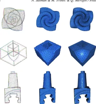
Figure 7: Feature preserving mesh generation on synthetic data

sets. From left to right: Our extracted polylines overlayed to the input point cloud; Delaunay refinement mesh of the Poisson im-plicit surface; output of our feature preserving mesh generation. Top: octa-flower; middle: carved_object (courtesy of P. Jenke); and bottom: blade models

recover sharp edges from sparse samplings (≤ 50k points). Notice, that in the case of carved_object and blade, the orig-inal models are 3D meshes, but the vertices of those meshes areNOTlying on the feature lines. The initial triangle edges are zigzaggy along the feature lines.

As already mentioned, our goal is to improve the accuracy for a given mesh size, by ensuring a faithful representation of sharp edges. To illustrate our achievement with repect to this goal, we show, for each model in Figure7, two meshes computed with the same value or parameter δ, hence the same value of Delaunay refinement algorithm parameters (α = 25◦

, l = 2 ∗ d′, d = 0.6 ∗ d′).

For quantitative evaluation of the accuracy improvement, Figure8shows an approximation of the Hausdorff distance between generated meshes and the ground truth model for various size of the generated mesh. Note that, the feature preserving Delaunay refinement (FPE) always outperforms standard Delaunay refinement (PIF) and that the effect is all the more important for coarse meshes.

Figure9is another illustration of the ability of our method to enhance the trade-off between accuracy and mesh size through feature extraction and preservation. Note that the only way for standard mesh generation methods (marching cubes and Delaunay” refinement) to overcome the lack of feature lines is to generate high resolution meshes.

Complex datasets.In order to evaluate the ability of our feature extraction method to cope with noise, we perturbed

(a) f andisk (b) block

Figure 8: Quantitative evaluation of the accuracy versus mesh size :

(a) the fandisk model, points on the curve correpond to values 10, 7, 4.5 and 3.5 ofδ (b) the block model, points on the curve correpond to

values 9, 6, 3 and 1.5 ofδ. The Hausdorff distance plotted vertically

is given in units of₂₀₀1 of the bounding box diagonal length.

the points sampled on the fandisk model. The perturbation is uniform and has an amplitude of 1% of the diagonal of the dataset bounding box. Keeping the same set of parame-ters (t1,t2) as for the unperturbed fandisk model, Figure10

shows the detected edge points. Although the edge points are more diffused with this amount of noise, the computed fea-ture directions remain quite stable. Moreover, despite intro-ducing strong noise, the feature extraction step constructed almost all sharp edges.

To evaluate the practical usability of this new approach, we applied it to two laser scan datasets acquired from two differ-ent environmdiffer-ents. The first one is an indoor laser acquisition of the Ramses model, Figure11. The second is an outdoor laser acquisition of the Church of Lans le Villard (France), Figure12. These datasets pose some problems compared to the synthetic models presented previously as near sharp fea-tures data are sparse and entangled with a high level of noise. The total time required to construct the feature polylines de-pends on the number of detected sharp edges points. Our prototype program has not been optimized and the details

Model/ Parameters |F | Timings [sec]

#points t1, t2, δ (1) (2) (3) (4) Fig. fandisk/200k 50, 6, 3.5 2k 153 17 20 24 6 50, 6, 7 2k 153 17 20 7 6 noise 1% 50, 6, 7 3k 126 32 41 7 10 octa-flower/167k 25, 4, 3.5 3k 96 19 53 13 7 carved_object/30k 16, 4, 4 2k 18 13 18 12 7 blade/50k 100, 7, 2.5 4k 34 52 32 9 7 block/40k 8, 2, 6 2k 16 20 37 7 9 Ramses/210k 150, 7, 5 8k 108 112 67 17 11 Lans church/500k 90, 10, 5 17k 368 306 184 78 12

Table 1: Statistics of our prototype implementation. The timings are

given for each of the 4 stages in our method: sharp edges points detection (1); clustering (2); polyline construction and junction (3); and feature preserving mesh generation (4).

Figure 9: From left to right: input point cloud and overlayed extracted feature polylines for the block model and three generated meshes from

the implicit surface obtained by Poisson reconstruction: marching cubes implementation [KBH06], with default octree depth, (62k facets); standard Delaunay refinement [BO05], withδ = 0.5, (60k facets); our feature preserving Delaunay refinement, with δ = 6, (900 facets).

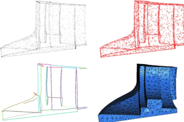
Figure 10: Feature extraction and preserving mesh generation for

the fandisk model corrupted with uniform noise of1% of its

bound-ing box. From top to bottom, left to right: the detected edge points

(t1= 50,t2= 6); the associated feature directions; the extracted

feature polylines; the output mesh with(δ = 7). Note how

choos-ing large protective balls patches the small gaps (pointed by small arrows) between feature polylines.

shown in Table1are just given for indication (on a laptop with 3.5Gb memory, Intel CoreR TM2 2.7Ghz processor). Limitations. Since feature extraction and smooth surface reconstruction are run independently, the extracted feature graph may have a certain discrepancy with respect to the smooth reconstructed surface. The feature preserving mesh generation algorithm yields a surface mesh with a faithfull representation of sharp features provided that the protecting balls cover the gap between the extracted features and the reconstructed smooth surface. This condition puts one more constraint on the parameter δ and, hence on the mesh accu-racy and sizing.

The pipeline currently described does not support adaptative sampling and the generation of meshes with non uniform siz-ing field. This however is not a real limitation of the method

Figure 11: Left: input point cloud of Ramses model downsampled to

about 27% of the original dataset (top), extracted feature polylines (bottom). Middle: meshed Poisson implicit function. Right: output of our feature preserving mesh generation (5k facets).

but simply results from our concern to limit and simplify the parameters of the algorithm.

5 Conclusion

In this paper, we have presented an efficient and robust feature preserving mesh generation strategy from 3D point clouds. The approach we use builds a bridge between im-plicit surface reconstruction and mesh generation.

As for future work, it would be interesting to explore the pos-sibility to automatically pre-compute the different parame-ters from the input point cloud. We are also planning to ex-ploit the mesh generation algorithm flexibility to apply our method to more challenging datasets provided by multi-view stereo reconstruction. We also plan to make our code avail-able very soon and we hope that it will be useful in the fields which require simplified and realistic geometric models, like in urban modelling.

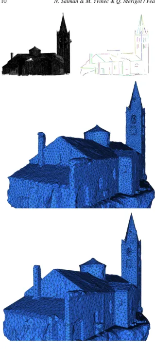
Figure 12: From top to bottom, left to right: input point cloud of

Church model (courtesy of INPG) downsampled to about 7.2% of the original dataset; extracted feature polylines; meshed Poisson implicit function; output of our feature preserving mesh generation.

Acknowledgements

We wish to express our thanks to the reviewers for their insightful comments. We also thank Pierre Alliez for the precious discussions, Stephane Tayeb and Laurent Rineau to provide access to their ex-perimental meshing code, Joel Daniels and the Aim@Shape reposi-tory for the several data-sets. This work was partially supported by the ANR (Agence Nationale de la Recherche) under the “Gyroviz” project (No ANR-07-AM-013)www.gyroviz.organd by the Fon-dation d’entreprise EADS, contract no 3610.

References

[AA06] ADAMSONA., ALEXAM.: Anisotropic point set sur-faces. In Proc. of Afrigraph ’06 (2006), p. 13.

[AB99] AMENTA N., BERN M.: Surface reconstruction by Voronoi filtering. Discrete and Computational Geometry 22 (1999), 481–504.

[ann] ANN, a library for Approximate Nearest Neighbor search-ing. http://www.cs.umd.edu/ mount/ANN/.

[BO05] BOISSONNATJ., OUDOTS.: Provably good sampling and meshing of surfaces. Graphical Models 67, 5 (2005), 405– 451.

[CDL07] CHENGS., DEYT., LEVINEJ.: A Practical Delaunay Meshing Algorithm for a Large Class of Domains*. In Proc. of

IMR ’07(2007), Springer, pp. 477–494.

[CDR07] CHENGS.-W., DEYT. K., RAMOSE. A.: Delaunay refinement for piecewise smooth complexes. In Proc. of SODA

’07(2007), pp. 1096–1105.

[cga] CGAL, Computational Geometry Algorithms Library. http://www.cgal.org.

[DHOS07] DANIELSJ. I., HAL. K., OCHOTTAT., SILVAC. T.: Robust smooth feature extraction from point clouds. In Proc. of

SMI ’07(2007), pp. 123–136.

[DTS01] DINHH., TURK G., SLABAUGHG.: Reconstructing

surfaces using anisotropic basis functions. In Proc. of ICCV ’01 (2001), pp. 606–613.

[ES97] EDELSBRUNNERH., SHAHN.: Triangulating Topologi-cal Spaces. International Journal of Computational Geometry &

Applications 7, 4 (1997), 365–378.

[FCOS05] FLEISHMANS., COHEN-OR D., SILVAC.: Robust

moving least-squares fitting with sharp features. In Proc. of ACM

SIGGRAPH ’05(2005), p. 552.

[GG07] GUENNEBAUDG., GROSSM.: Algebraic point set sur-faces. In Proc. of ACM SIGGRAPH ’07 (2007), p. 23.

[HDD∗_{92] HOPPEH., DEROSET., DUCHAMPT., MCDONALD}

J., STUETZLE W.: Surface reconstruction from unorganized points. Proc. of ACM SIGGRAPH ’92 (1992), 71–71.

[JWSA08] JENKE P., WAND M., STRASSER W., AKA A.: Patch-graph reconstruction for piecewise smooth surfaces. Proc.

of VMV ’08(2008), 3.

[KBH06] KAZHDANM., BOLITHOM., HOPPEH.: Poisson Sur-face Reconstruction. In Proc. of SGP ’06 (2006), pp. 61–70. [KBSS01] KOBBELTL., BOTSCHM., SCHWANECKEU., SEI

-DELH.: Feature sensitive surface extraction from volume data. In Proc. of ACM SIGGRAPH ’01 (2001), pp. 57–66.

[LCOL07] LIPMAN Y., COHEN-OR D., LEVIN D.: Data-dependent MLS for faithful surface approximation. In Proc. of

SGP ’07(2007), p. 67.

[Lee00] LEEI.: Curve reconstruction from unorganized points.

Computer Aided Geometric Design 17, 2 (2000), 161–177.

[MOG09] MÉRIGOTQ., OVSJANIKOV M., GUIBASL.: Ro-bust voronoi-based curvature and feature estimation. In Proc.

of SIAM/ACM SPM ’09(2009), pp. 1–12.

[OBA∗_{03] OHTAKE Y., BELYAEVA., ALEXAM., TURKG.,}

SEIDELH.: Multi-level partition of unity implicits. In Proc.

of ACM SIGGRAPH ’03(2003), pp. 463–470.

[OBA05] OHTAKEY., BELYAEVA., ALEXAM.: Sparse low-degree implicit surfaces with applications to high quality ren-dering, feature extraction, and smoothing. In Proc. of SGP ’05 (2005), p. 149.

[OGG] OZTIRELIC., GUENNEBAUDG., GROSS M.: Feature preserving point set surfaces based on non-linear kernel regres-sion. In Computer Graphics Forum.

[PKG03] PAULYM., KEISERR., GROSSM.: Multi-scale feature extraction on point-sampled surfaces. In Computer Graphics

Fo-rum(2003), vol. 22, pp. 281–289.

[She00] SHEWCHUKJ.: Mesh generation for domains with small

angles. In Proc. of SCG ’00 (2000), p. 10.

[SSFS06] SCHREINER J., SCHEIDEGGER C., FLEISHMAN S., SILVAC.: Direct (re) meshing for efficient surface processing. In Computer Graphics Forum (2006), vol. 25, pp. 527–536.