Analysis of Frequency-Smearing Models
Simulating Hearing Loss
by
Alan T. Asbeck
Submitted to the Department of Electrical Engineering and Computer
Science
in Partial Fulfillment of the Requirements for the Degree of
Master of Engineering in Electrical Engineering and Computer Science
at the Massachusetts Institute of Technology
May 21, 2003
Copyright 2003 M. I. T. All rights reserved.
MASSACHUSETTS INSTITUTE OFTECHNOLOGY
UL 302003
LIBRARIES
Author
Department of Nfectrical Engineering and Computer Science
May 21, 2003
Certified by...
...
.
Louis D. Braida
Henry Ellis Warren Professor of Electrical Engineering
Thesis Supervisor
Accepted by ... ...
Arthur C. Smith
Chairman, Department Committee on Graduate Theses
Analysis of Frequency-Smearing Models Simulating Hearing
Loss
by
Alan T. Asbeck
Submitted to the Department of Electrical Engineering and Computer Science on May 21, 2003, in partial fulfillment of the
requirements for the degree of
Master of Engineering in Electrical Engineering and Computer Science
Abstract
Various authors have created models of the psychoacoustic effects of sensorineural hearing loss that transform ordinary sounds into sounds that evoke the perception of hearing loss in normal-hearing listeners. In this thesis, models of the reduced frequency resolution, reduced temporal resolution, and loudness recruitment and absolute threshold loss were evaluating using a model of human perception. Confusion matrices of vowels were simulated using these models and compared to confusion matrices from five hearing-impaired subjects. It was found that the model of human perception used spectral cues in a different way than actually occurs in humans, making it difficult to evaluate the hearing loss models, and causing the simulated confusion matrices to be different than the real subjects' matrices. Even so, the frequency smearing models caused the total error rate to increase with increasing smearing bandwidth, and the results were generally consistent with the expected behavior.
Thesis Supervisor: Louis D. Braida
Acknowledgments
I first want to thank my advisor, Professor Louis Braida, for his help and support throughout this project, and for giving me a project in the first place. I especially want to thank him for putting up with my tendency to procrastinate, and for spending so much time reading my thesis and being there at the end.
I want to thank Michael "Q" Chin, for really making my time here a wonderful experience, and for helping me think through this project and other things throughout the year. I've really appreciated the time we've been able to get to know each other, including everything from the "sea-snakes" on the chalkboard and talking about the various topics you have come up with.
I also want to thank Peninah Rosengard, Charlotte Reed, Andrew Oxenham, and everyone else in the Sensory Communication group that has helped me along the way. Finally, I acknowledge the NIH and NSF, which have provided funding for my work on this thesis.
Contents
1 Introduction
1.1 Background . . . . 1.2 Physiology of Hearing Impairment . . . . 1.3 Psychoacoustics of Hearing Impairment . . . . . 1.4 Simulating Hearing Loss . . . . 1.4.1 Reasons for Simulating Hearing Loss . . 1.4.2 Previous Work Simulating Hearing Loss 1.5 Problem Statement . . . .
2 Signal Processing in the Experiment
2.1 Overview of Experiment . . . . 2.2 Overview of Signal Processing . . . . 2.2.1 Processing by Real Subjects . . . . 2.2.2 Processing by the Simulation . . . . 2.3 Detail on the Brantley Confusion Matrix Experiment . . . 2.4 Speech Stimuli and Vowel Extraction . . . . 2.5 Signal processing simulating hearing loss . . . . 2.5.1 Methods of frequency smearing . . . . 2.5.2 Method of Recruitment . . . . 2.5.3 Combining the Smearing Methods and Recruitment
2.6 d' Discrimination Model . . . . 25 . . . . 25 . . . . 25 . . . . 28 . . . . 31 . . . . 31 . . . . 32 . . . . 35 36 36 . . . . . 37 . . . . . 37 . . . . . 37 . . . . . 40 . . . . . 41 . . . . . 42 42 . . . . . 61 . . . . . 71 . . . . . 71
3 Results 78
3.1 Total Error Rates . . . . 78
3.2 Locations of Errors in Confusion Matrices . . . . 79
3.2.1 Comparison of Moore and ter Keurs Methods . . . . 84
3.3 Effects of Processing Parameters on the Results . . . . 85
3.3.1 Loudness recruitment and Audibility . . . . 85
3.3.2 Male vs. Female Speakers . . . . 86
3.4 Results with Simulating Full Audibility . . . . 87
3.4.1 Error rates . . . . 88
3.4.2 Locations of Errors . . . . 89
3.4.3 Comparison of Moore and ter Keurs Methods . . . . 89
4 Discussion 118 4.1 Why the Simulation Did Not Work . . . . 118
4.2 Other Sources of Error . . . . 122
4.3 Conclusions that Can Be Drawn . . . . 122
4.3.1 Total Error Rates and Smearing and Recruitment . . . . 123
4.3.2 Comparing Moore and ter Keurs Smearing . . . . 126
4.3.3 The Effect of Audibility . . . . 127
4.4 Potential Perceptual Models in Humans . . . . 128
5 Conclusions 132 5.1 Summary of Findings . . . . 132
5.2 Relevance to Hearing Aid Signal Processing . . . . 133
5.3 Recommendations for Future Work . . . . 133
A Audiograms and Confusion Matrices for the Real Subjects 135
B Tables of Computed Confusion Matrices 140
D Recommendations for an Improved Simulation 183
D.1 Rationale and Background ... 183
D.2 Overview of Model . . . . 183
D .3 Details of M odel . . . . 184
D.4 Simulating Hearing Loss . . . . 186
D.5 Possible Sources of Error . . . . 187
List of Figures
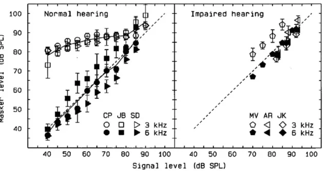
1-1 Figure showing how the basilar membrane is compressive for tones at the best frequency of the location of measurement. This figure shows "the level of a masker required to mask [a] 6-kHz [tone] signal, as a function of signal level" (Oxenham and Plack, 1997). The plot of the on-frequency masker is linear, as would be expected. However, the off-frequency masker shows compression, indicating both that the basilar membrane is compressive and that it responds linearly for tones an octave below the best frequency of a given location. Taken from Oxenham and Plack, 1997. . . . . 27 1-2 Loudness matching curves for subjects with unilateral hearing loss.
The thin line at a 45-degree angle is the expected result if the two ears gave equal loudness results for a tone at a given level. The fact that the actual data is at a steeper slope than this indicates that for the impaired ear, as the stimulus sound pressure level increases a little, the apparent loudness increases more rapidly than in a normal ear. Also, the asterisks indicate the subjects' absolute thresholds; these are elevated in the impaired ear relative to the normal ear. Taken from Moore et al., 1996, with the 45-degree line added. . . . . 30
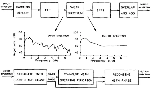
2-2 Block diagrams of Moore frequency smearing algorithm. The top block diagram shows the main processing sequence, and the bottom block diagram shows detail for the "Smear Spectrum" block in the top part. Taken from Baer and Moore, 1993. . . . . 44 2-3 Spectra resulting from different amounts of Moore smearing on the
vowel II taken from the word BIIDH. All files were put through the recruitment algorithm but with no recruitment. The unsmeared signal is shown at the regular level, while the other traces have been offset by -40 dB increments. The labels to the left of the traces indicate the amount of smearing, in terms of the effective number of ERBs of the widened auditory filters; US indicates the unsmeared signal. . . . . . 47 2-4 Channels resulting from different amounts of Moore smearing on the
vowel II taken from the word BIIDH. All files were put through the recruitment algorithm but with no recruitment. The unsmeared signal is shown at the regular level, while the other traces have been offset by -8 dB increments. The labels to the left of the traces indicate the amount of smearing, in terms of the effective number of ERBs of the widened auditory filters; US indicates the unsmeared signal. . . . . . 48 2-5 Sample spectra showing the results of smearing, for a synthetic vowel
/ae/.
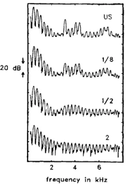
The different frames (vertical dimension in the figure) show successive chunks of signal that are partially overlapping. As can be seen in the right column, showing the output spectra, the effective degree of smearing is less than was intended. The intended degree of smearing is seen in the middle column, which shows the results after smearing but before the overlap-add process. Taken from Baer and M oore, 1993. . . . . 50 2-6 Block diagram showing the details of the ter Keurs processing method.2-7 Block diagram showing the details of the Spectral Smearing block from 2-6. Taken from ter Keurs et al., 1992. . . . . 53 2-8 Sample of the outputs of the ter Keurs frequency smearing algorithm.
The top log spectrum, labeled "US," shows the unsmeared signal, while the bottom three spectra show the results of smearing of 1/8, 1/2, and 2 octaves, as labeled. Taken from ter Keurs et al., 1992 . . . . 54 2-9 Spectra resulting from different amounts of ter Keurs smearing on the
vowel II taken from the word BIIDH. All files were put through the recruitment algorithm but with no recruitment. The unsmeared signal is shown at the regular level, while the other traces have been offset by -50 dB increments. The labels to the left of the traces indicate the amount of smearing, in octaves; US indicates the unsmeared signal. One octave of smearing is approximately equivalent to 3.9 ERBs of sm earing. . . . . 55 2-10 Channels resulting from different amounts of ter Keurs smearing on the
vowel II taken from the word BIIDH. All files were put through the recruitment algorithm but with no recruitment. The unsmeared signal is shown at the regular level, while the other traces have been offset by -12 dB increments. The labels to the left of the traces indicate the amount of smearing, in octaves; US indicates the unsmeared signal. One octave of smearing is approximately equivalent to 3.9 ERBs of sm earing. . . . . 56 2-11 Block diagram of perceptual model of human temporal processing, used
by Hou and Pavlovic in providing rationale for their temporal smearing model. Taken from Hou and Pavlovic, 1994. . . . . 58 2-12 Block diagram of the Hou temporal smearing model. The top diagram
(a) shows the overall signal processing path, and the bottom diagram (b) shows the specifics of how temporal smearing is accomplished. Figure reproduced from Hou and Pavlovic, 1994. . . . . 59
2-13 Sample of outputs from the Hou temporal smearing model. The top panels (a and b) show the unsmeared signal and its spectrum, and the lower panels show the signal and its spectrum after it has been smeared with an ERD of 0.lms and 28ms, respectivley. Figure taken from Hou and Pavlovic, 1994. . . . . 62 2-14 Spectra resulting from different amounts of Hou smearing on the
vowel II taken from the word BIIDH. All files were put through the recruitment algorithm but with no recruitment. The unsmeared signal is shown at the regular level, while the other traces have been offset by -50 dB increments. The labels to the left of the traces indicate the amount of smearing, that is, the equivalent rectangular duration of the smearing temporal window, in msec; US indicates the unsmeared signal. 63 2-15 Channels resulting from different amounts of Hou smearing on the
vowel II taken from the word BIIDH. All files were put through the recruitment algorithm but with no recruitment. The unsmeared signal is shown at the regular level, while the other traces have been offset by -8 dB increments. The labels to the left of the traces indicate the amount of smearing, that is, the equivalent rectangular duration of the smearing temporal window, in msec; US indicates the unsmeared signal. 64 2-16 Block diagram of the model of loudness recruitment by Moore and
Glasberg, 1993. The parallel arrows between the middle blocks represent the outputs of the 23 bandpass filters in the first block. Figure taken from Moore and Glasberg, 1993. . . . . 65
2-17 Channels resulting from different amounts of recruitment on the vowel II taken from the word BIIDH. The vowel was at a level of 100 dB. Recruitment of N = 1.0 (where N is the exponent to which the envelope is taken) corresponds to a hearing loss of 0 dB, recruitment of N = 2.0 corresponds to a flat hearing loss of 50 dB, and in general the recruitment amounts correspond to hearing losses via the equation
N = lOOdB/(1OOdB - hearinglossdB). No additional offsets were
used in creating the plot: the effective level changes with increasing recruitment due to the increased absolute threshold. . . . . 68 2-18 Channels resulting from different amounts of recruitment on the vowel
II taken from the word BIIDH. The vowel was at a level of 80 dB. Recruitment of N = 1.0 (where N is the exponent to which the envelope is taken) corresponds to a hearing loss of 0 dB, recruitment of N = 2.0 corresponds to a flat hearing loss of 50 dB, and the other recruitment amounts correspond to hearing losses via the equation N = lOOdB/(1OOdB - hearinglossdB). No additional offsets were
used in creating the plot: the effective level changes with increasing recruitment due to the increased absolute threshold. . . . . 69
2-19 Channels resulting from different amounts of recruitment on the vowel II taken from the word BIIDH. The solid lines are the result of recruitment with a simulated loss of 0 dB, and the dotted lines are the result of recruitment with a flat loss of 50 dB. The dashed line shows channels made from the original signal without recruitment, showing that simulating a loss of 0 dB does not distort the signal very much. Signals with levels of 120, 100, and 80 dB were recruited corresponding to losses of 0 dB and 50 dB, creating pairs of lines for each signal level. The 120 dB signal is above 100 dB the limit of recruitment, so recruitment has little effect. The 100 dB signal has the highest parts at around the limit of recruitment, so they are not affected, while the higher frequency portions of the signal are lower in level and so are distorted. The 80 dB signal is severely distorted and reduced in level by recruitm ent. . . . . 70 2-20 Block diagram of d' discrimination model. The bottom block comes
after the top block in the processing path. The top block is used to create channels from all vowels processed, and the bottom block takes all combinations of pairs of vowels, and produces a d' distance between each pair. In the top figure, the signal is first filtered into bands. Then, in each band, the average power per unit length of the signal is found by first squaring it, summing over the signal length, dividing by the signal length, and then normalizing to account for variation in signal length between stimuli. Finally, the natural log of the resulting number is taken to produce a channel. In the bottom diagram, the difference (Ai) between corresponding channels is found for a pair of stimuli, as indicated in the plot. These differences are then put through the formula in the bottom of the figure. E is an arbitrary constant that is a scale factor for all d' distances . . . . 73
2-21 Illustration of decision model function in two dimensions. Stimulus centers are represented by the small points in the figure, and are surrounded by Gaussian distributions in perceptual space. Response centers are found by taking the centroid of the stimulus centers of a single type. The probability distributions around each stimulus center are assumed to evoke responses corresponding to the closest response center. The lines dividing the figure are the boudaries of these so-called response regions. . . . . 76 2-22 Block diagram of decision model. . . . . 77
3-1 Total error rates for the simulation using subject JB's audiogram. Solid lines indicate results with just smearing and no recruitment, as indicated in the legend, and dotted lines indicate those conditions followed by recruitment. The dashed line is subject JB's actual error
rate. ... ... 94
3-2 Total error rates for the simulation using subject JO's audiogram. Solid lines indicate results with just smearing and no recruitment, as indicated in the legend, and dotted lines indicate those conditions followed by recruitment. The dashed line is subject JO's actual error
rate. ... ... 95
3-3 Total error rates for the simulation using subject MG's audiogram. Solid lines indicate results with just smearing and no recruitment, as indicated in the legend, and dotted lines indicate those conditions followed by recruitment. The dashed line is subject MG's actual error rate. .... ... ... ... . .. 96 3-4 Total error rates for the simulation using subject PW's audiogram.
Solid lines indicate results with just smearing and no recruitment, as indicated in the legend, and dotted lines indicate those conditions followed by recruitment. The dashed line is subject PW's actual error
3-5 Total error rates for the simulation using subject RC's audiogram. Solid lines indicate results with just smearing and no recruitment, as indicated in the legend, and dotted lines indicate those conditions followed by recruitment. The dashed line is subject RC's actual error
rate. ... ... ... ... 98
3-6 Error rates relative to the total error rate for unsmeared stimuli for the simulation using subject JB's audiogram. Solid lines indicate results with just smearing and no recruitment, as indicated in the legend, and dotted lines indicate those conditions followed by recruitment. The dashed line is subject JB's actual error rate. . . . . 99 3-7 Error rates relative to the total error rate for unsmeared stimuli for the
simulation using subject JO's audiogram. Solid lines indicate results with just smearing and no recruitment, as indicated in the legend, and dotted lines indicate those conditions followed by recruitment. The dashed line is subject JO's actual error rate. . . . . 100 3-8 Error rates relative to the total error rate for unsmeared stimuli for the
simulation using subject MG's audiogram. Solid lines indicate results with just smearing and no recruitment, as indicated in the legend, and dotted lines indicate those conditions followed by recruitment. The dashed line is subject MG's actual error rate. . . . . 101 3-9 Error rates relative to the total error rate for unsmeared stimuli for the
simulation using subject PW's audiogram. Solid lines indicate results with just smearing and no recruitment, as indicated in the legend, and dotted lines indicate those conditions followed by recruitment. The dashed line is subject PW's actual error rate. . . . . 102
3-10 Error rates relative to the total error rate for unsmeared stimuli for the simulation using subject RC's audiogram. Solid lines indicate results with just smearing and no recruitment, as indicated in the legend, and dotted lines indicate those conditions followed by recruitment. The dashed line is subject RC's actual error rate. . . . 103 3-11 Plot showing how well the average of all of the confusion matrix data
fit to the subject's actual confusion matrices. Averages were taken across all subjects and smearing amounts, for the reduced-audibility sim ulation. . . . 104 3-12 A comparison of the ter Keurs results (dotted line) and Moore results
(solid line) if the total error rates are approximately the same for the two smearing conditions. The ter Keurs result had a smearing multiplier of 1.0, and the Moore smearing had a multiplier of 1.5. For each pair of ter Keurs and Moore values (plotted in the same vertical space), the subject used to create the simulated matrix and the real subject it was being compared to were the same. . . . 105 3-13 A comparison of the ter Keurs results (dotted line) and Moore results
(solid line) if the total error rates are approximately the same for the two smearing conditions. The ter Keurs result had a smearing multiplier of 1.5, and the Moore smearing had a multiplier of 2.0. For each pair of ter Keurs and Moore values (plotted in the same vertical space), the subject used to create the simulated matrix and the real subject it was being compared to were the same. . . . 106
3-14 Graph showing the percentage of stimuli that had audible channels for a given channel number, for each subject. Note that the channels correspond to a log scale with channel 1 centered at 100 Hz, channel 12 at 1575 Hz, and channel 19 at 4839 Hz (for reference). Also, it can be seen that in most plots two groups of curves can be seen. The set of curves to the left corresponds to no recruitment, and the set to the right is with recruitment. . . . 107 3-15 Plot showing the stimulus centers and response centers for the stimuli
from the male and female speakers combined (top plot), and just the female speaker (bottom plot). The stimulus centers are shown by the small black dots, and the response centers are shown by the open circles. In each plot, the response centers are the average of the stimulus centers for each vowel. Only half of the total number of stimulus centers were plotted for computational reasons. As can be seen around the "AH" in the top plot, the stimuli corresponding to the male and female speakers formed two distinct clusters for each vowel. The clusters are not distinct for the other vowels in this plot due to the perspective. Also, it can be seen that the stimulus centers for each vowel are less spread out in the bottom plot. . . . 108 3-16 Plot showing how well the average of all of the confusion matrix data
fit to the subject's actual confusion matrices. Averages were taken across all subjects, with the smearing multiplier fixed at 1.0, for the reduced-audibility simulation. . . . 109 3-17 Total error rates for the simulation using subject JB's audiogram,
assuming that all frequencies are audible to the subject. Solid lines indicate results with just smearing and no recruitment, as indicated in the legend, and dotted lines indicate those conditions followed by recruitment. The dashed line is subject JB's actual error rate. . . . . 110
3-18 Total error rates for the simulation using subject JO's audiogram, assuming that all frequencies are audible to the subject. Solid lines indicate results with just smearing and no recruitment, as indicated in the legend, and dotted lines indicate those conditions followed by recruitment. The dashed line is subject JO's actual error rate. . . . . 111 3-19 Total error rates for the simulation using subject MG's audiogram,
assuming that all frequencies are audible to the subject. Solid lines indicate results with just smearing and no recruitment, as indicated in the legend, and dotted lines indicate those conditions followed by recruitment. The dashed line is subject MG's actual error rate. . . . . 112 3-20 Total error rates for the simulation using subject PW's audiogram,
assuming that all frequencies are audible to the subject. Solid lines indicate results with just smearing and no recruitment, as indicated in the legend, and dotted lines indicate those conditions followed by recruitment. The dashed line is subject PW's actual error rate. . . . . 113 3-21 Total error rates for the simulation using subject RC's audiogram,
assuming that all frequencies are audible to the subject. Solid lines indicate results with just smearing and no recruitment, as indicated in the legend, and dotted lines indicate those conditions followed by recruitment. The dashed line is subject RC's actual error rate. . . . . 114 3-22 Plot showing how well the average of all of the confusion matrix data
fit to the subject's actual confusion matrices. Averages were taken across all subjects and smearing amounts, for the simulation in which all frequencies were audible. . . . 115
3-23 Assuming full audibility, a comparison of the ter Keurs results (dotted line) and Moore results (solid line) if the total error rates are approximately the same for the two smearing conditions. The ter Keurs result had a smearing multiplier of 1.0, and the Moore smearing had a multiplier of 1.5. For each pair of ter Keurs and Moore values (plotted in the same vertical space), the subject used to create the simulated matrix and the real subject it was being compared to were the same. 116 3-24 Assuming full audibility, a comparison of the ter Keurs results (dotted
line) and Moore results (solid line) if the total error rates are approximately the same for the two smearing conditions. The ter Keurs and Moore results both had a smearing multiplier of 2.0. For each pair of ter Keurs and Moore values (plotted in the same vertical space), the subject used to create the simulated matrix and the real subject it was
being compared to were the same. . . . 117
4-1 Average vowel lengths for the different vowels. The error bars represent one standard deviation of the vowel length. The averages were nearly identical for male and female speakers. . . . 130
4-2 Examples of spectra. In both cases, the d' discrimination algorithm will produce equal d' distances between all stimuli. However, a real human listener could easily distinguish that the third spectrum was much different than the other two. In Stimulus Set A, the spectrum heights are A, 2A, and A, for spectra 1,2, and 3, respectively. The widths of the spectra are such that the total area under all of the spectra is the sam e. . . . 131
A-1 Audiogram for subject PW. . . . 135
A-2 Audiograms for subjects JB and JO. . . . 136
C-2 C-3 C-4 C-5 C-6 C-7 C-8 C-9 C-10 C-11
Original simulation including reduced Original simulation including reduced Original simulation including reduced Original simulation including reduced Original simulation including reduced Original simulation including reduced Original simulation including reduced Original simulation including reduced Original simulation including reduced Original simulation including reduced C-12 Original simulation including reduced C-13 Original simulation including reduced C-14 Original simulation including reduced C-15 Original simulation including reduced C-16 All frequencies audible condition. C-17 All frequencies audible condition. C-18 All frequencies audible condition. C-19 All frequencies audible condition. C-20 All frequencies audible condition. C-21 All frequencies audible condition. C-22 All frequencies audible condition. C-23 All frequencies audible condition. C-24 All frequencies audible condition. C-25 All frequencies audible condition. .
C-26 All frequencies audible condition. .
C-27 All frequencies audible condition. .
C-28 All frequencies audible condition. .
C-29 All frequencies audible condition. .
C-30 All frequencies audible condition. .
audibility. ... 154 audibility. ... 155 audibility. . . . . 156 audibility. . . . . 157 audibility. . . . . 158 audibility. . . . . 159 audibility. . . . . 160 audibility. . . . . 161 audibility. . . . . 162 audibility. . . . . 163 audibility. . . . . 164 audibility. . . . . 165 audibility. . . . . 166 audibility. . . . . 167 . . . . 168 . . . . 169 . . . . 170 . . . . 17 1 . . . . 172 . . . . 173 . . . . 174 . . . . 175 . . . . 176 . . . . 177 . . . . 178 . . . . 179 . . . . 180 . . . . 18 1 . . . . 18 2
List of Tables
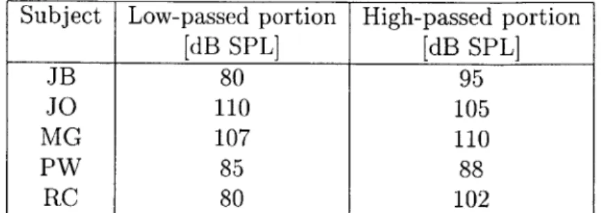
2.1 Table of the levels at which the low-passed (below 2500 Hz) and high-passed (above 2500 Hz) portions of the CVC syllables were presented to the subjects in the confusion matrix experiment by Brantley (1990-1991). 41
2.2 Table of the different processing conditions used in the simulation. . . 71 3.1 Table of the average simulated confusion matrices for each processing
condition. Averages were taken across subjects and smearing amounts. From top to bottom, the processing conditions are: No smearing, Moore smearing, ter Keurs smearing, and Hou smearing. The left column contains the results of smearing without recruitment, and the right column contains the results of smearing followed by recruitment. 83 3.2 Table of the simulated confusion matrices for approximately equivalent
total smearing amounts for the Moore and ter Keurs methods, without recruitment. The results shown in the table are the averages across all subjects. The top row contains a Moore smearing with a widening factor of 4.5, and ter Keurs smearing of 0.75 octaves. The total error rate with that amount of smearing for the Moore method was a little lower than the total error rate for that amount of ter Keurs smearing. The bottom row contains a Moore smearing with a widening factor of 6, and ter Keurs smearing of 1.125 octaves. The total error rate with that amount of smearing for the Moore method was a little higher than the total error rate for that amount of ter Keurs smearing. . . . . 85
3.3 Table of the average simulated confusion matrices for each processing condition. Averages were taken across subjects for a smearing multiplier of 1. From top to bottom, the processing conditions are: No smearing, Moore smearing, ter Keurs smearing, and Hou smearing. The left column contains the results of smearing without recruitment, and the right column contains the results of smearing followed by recruitm ent. . . . . 91 3.4 Table of the average simulated confusion matrices for each processing
condition, assuming that all frequencies are audible. Averages were taken across subjects and smearing amounts. From top to bottom, the processing conditions are: No smearing, Moore smearing, ter Keurs smearing, and Hou smearing. The left column contains the results of smearing without recruitment, and the right column contains the results of smearing followed by recruitment. . . . . 92 3.5 Table of the simulated confusion matrices for approximately equivalent
total smearing amounts for the Moore and ter Keurs methods, without recruitment, assuming that all frequencies are audible. The results shown in the table are the averages across all subjects. The top row contains a Moore smearing with a widening factor of 4.5, and ter Keurs smearing of 0.75 octaves. The total error rate with that amount of smearing for the Moore method was a somewhat (~5%) lower than the total error rate for that amount of ter Keurs smearing. The bottom row contains a Moore smearing with a widening factor of 6, and ter Keurs smearing of 1.5 octaves. The total error rate with that amount of smearing for the Moore method was almost identical to the total error rate for that amount of ter Keurs smearing. . . . . 93 A.1 Confusion matrix for subject JB. . . . 138 A.2 Confusion matrix for subject JO. . . . 138
A.4 Confusion matrix for subject PW. . . . 139 A.5 Confusion matrix for subject RC. . . . 139 B.1 Confusion matrices for the simulation done with subject JB's
parameters. From top to bottom, for each row the smearing conditions were: No smearing, Moore sm. only, ter Keurs sm. only, Hou sm. only. The amount of smearing in each column was the "Smearing Mulitplier" times a 'standard amount of smearing' (see beginning of the appendix). 141 B.2 Confusion matrices for the simulation done with subject JB's
parameters.From top to bottom, for each row the smearing conditions were: Moore sm. then recruitment, ter Keurs sm. then recruitment, Hou sm. then recruitment, and just recruitment. The amount of smearing in each column was the "Smearing Mulitplier" times a
'standard amount of smearing' (see beginning of the appendix). . . . 142
B.3 Confusion matrices for the simulation done with subject JO's parameters. From top to bottom, for each row the smearing conditions were: No smearing, Moore sm. only, ter Keurs sm. only, Hou sm. only. The amount of smearing in each column was the "Smearing Mulitplier" times a 'standard amount of smearing' (see beginning of the appendix). 143 B.4 Confusion matrices for the simulation done with subject JO's
parameters.From top to bottom, for each row the smearing conditions were: Moore sm. then recruitment, ter Keurs sm. then recruitment, Hou sm. then recruitment, and just recruitment. The amount of smearing in each column was the "Smearing Mulitplier" times a
'standard amount of smearing' (see beginning of the appendix). . . . 144
B.5 Confusion matrices for the simulation done with subject MG's parameters. From top to bottom, for each row the smearing conditions were: No smearing, Moore sm. only, ter Keurs sm. only, Hou sm. only. The amount of smearing in each column was the "Smearing Mulitplier" times a 'standard amount of smearing' (see beginning of the appendix). 145
B.6 Confusion matrices for the simulation done with subject MG's parameters.From top to bottom, for each row the smearing conditions were: Moore sm. then recruitment, ter Keurs sm. then recruitment, Hou sm. then recruitment, and just recruitment. The amount of smearing in each column was the "Smearing Mulitplier" times a
'standard amount of smearing' (see beginning of the appendix). . . . 146
B.7 Confusion matrices for the simulation done with subject RC's parameters. From top to bottom, for each row the smearing conditions were: No smearing, Moore sm. only, ter Keurs sm. only, Hou sm. only. The amount of smearing in each column was the "Smearing Mulitplier" times a 'standard amount of smearing' (see beginning of the appendix). 147 B.8 Confusion matrices for the simulation done with subject RC's
parameters.From top to bottom, for each row the smearing conditions were: Moore sm. then recruitment, ter Keurs sm. then recruitment, Hou sm. then recruitment, and just recruitment. The amount of smearing in each column was the "Smearing Mulitplier" times a
'standard amount of smearing' (see beginning of the appendix). . . . 148
B.9 Confusion matrices for the simulation done with subject PW's parameters. From top to bottom, for each row the smearing conditions were: No smearing, Moore sm. only, ter Keurs sm. only, Hou sm. only. The amount of smearing in each column was the "Smearing Mulitplier" times a 'standard amount of smearing' (see beginning of the appendix). 149 B.10 Confusion matrices for the simulation done with subject PW's
parameters.From top to bottom, for each row the smearing conditions were: Moore sm. then recruitment, ter Keurs sm. then recruitment, Hou sm. then recruitment, and just recruitment. The amount of smearing in each column was the "Smearing Mulitplier" times a
Chapter 1
Introduction
1.1
Background
Due to the current state of technology, it is possible to do substantial signal processing in hearing aids. As such, the goal of hearing aid research is to come up with signal processing schemes to enable hearing-impaired individuals to experience sound as much as is possible like normal listeners, or at least to be able to consistently understand speech in various environments and at various levels. In order to develop said signal processing algorithms, it is necessary to understand how hearing-impared people experience sound, so that any differences can be accounted for. Thus, hearing aid research currently is largely focused on developing models of how hearing-impaired people experience sound. This chapter contains a discussion of the physiology of hearing impairment and the perceptual consequences of hearing loss to provide background for understanding the models, and also discusses previous work on hearing loss simulations.
1.2
Physiology of Hearing Impairment
The first stages of the auditory system include the outer, middle, and inner ear, after which the auditory nerve takes the resulting signals to the brain. The outer and
middle ear serve to collect and channel the sound into the head. The inner ear serves several functions: it acts as a sort of frequency analyzer, to separate the sound into different frequency bands; it amplifies the sound; and it converts the mechanical sound signal into neural signals. These functions take place within the inner ear structure known as the cochlea. The cochlea is essentially a coiled tube that is partitioned lengthwise by several membranes. One of these is known as the basilar membrane (BM), which is a stiff structure that performs the first stage of frequency analysis through its mechanical properties: it is about 100 times stiffer at the base (the place where the sound first encounters it) than at the apex (the other end from the base). This variable stiffness means that different locations on the BM will respond (oscillate) the best to different input frequencies: it acts as a frequency-to-place converter. The frequency that causes the maximum response of a particular location on the BM is known as the best frequency (BF) or characteristic frequency (CF) of that location. High frequencies to cause the basal end to be excited more, while low frequencies travel down the length of the BM and create more of a response toward the apical end.
Attached to the BM are rows of cells known as outer hair cells (OHCs). These cells serve primarily as mechanical transducers, actively causing the BM to vibrate even more in response to incoming sounds than it would on its own. This causes the BM to be even more frequency selective (that is, exhibit sharper tuning to tone stimuli) and causes the incoming sounds to be amplified. It has been found that due to the OHCs, the transfer function between the incoming sound level and the resulting BM oscillation displacement at a particular location is compressive for CF tones. This compression takes place for tones at input levels between about 30-90 dB SPL (Oxenham and Plack, 1997). A graph showing this transfer function is shown in figure 1-1. For tones that are an octave or more lower than the CF of a location on the BM, the BM responds linearly. This is also shown in figure 1-1.
40 50 60 70 80 90 100 Signal level Impaired hearing 40 (dB 50 60 SPL) 70 80 90 100
Figure 1-1: Figure showing how the basilar membrane is compressive for tones at the best frequency of the location of measurement. This figure shows "the level of a masker required to mask [a] 6-kHz [tone] signal, as a function of signal level" (Oxenham and Plack, 1997). The plot of the on-frequency masker is linear, as would be expected. However, the off-frequency masker shows compression, indicating both that the basilar membrane is compressive and that it responds linearly for tones an octave below the best frequency of a given location. Taken from Oxenham and Plack,
1997. 100 a_ cn (1) C-) Ut) XD 90 80 70 50 50 40 Normal hearing CP JB so6 0 0 [> 3 kHz 0 0 NO 5 k Hz AR 3 kHz 6 kHz MV JK 0
fibers, and act to convert the amplitude (or velocity) of BM oscillation into neural firing patterns. In response to frequencies below about 2 kHz, the IHCs cause spikes on the auditory nerve to be "phase-locked" to those frequencies, meaning that the spike trains are in phase with the BM motion caused by the signal, and the temporal patterns of the signal itself. At higher frequencies, auditory nerve fiber firing patterns are not phase-locked to the BM motion, meaning that their firing rate is not correlated with the signal.
When sensorineural hearing loss occurs, typically the OHCs and/or IHCs are damaged. This damage can occur in any location along the length of the cochlea, which translates to different frequency regions having different amounts of hearing loss due to the frequency-to-place transformation in the cochlea. IHC loss is primarily a conduction loss, as the IHCs act as sensors of the BM motion. This type of hearing loss can typically be corrected for by linear amplification of the incoming signal. However, in the majority of cases, OHC loss is the more dominant effect in hearing loss. The effect of OHC loss is that the sharp frequency tuning of the BM is lost in regions where there has been OHC damage, since the OHCs will no longer function as active amplifiers. Additionally, those regions of the cochlea do not have the gain in signal level caused by the OHCs. This means that compression will not take place to as large a degree. In cases of severe OHC loss, no compression or signal gain remains, and the BM responds linearly to the incoming sound waves.
The current experiment, and hearing aid research in general, are focused on studying the effects of hearing loss caused by OHC damage alone. The next section will discuss the perceptual consequences of this type of hearing loss.
1.3
Psychoacoustics of Hearing Impairment
In discussing the perceptual consequences of hearing loss, it will be helpful to first define some terms commonly used in discussing auditory perception. The first idea is
perception of the sound is examined, a good model for this transfer function is a filter bank of auditory filters. The specific form of the auditory filters will be described later, but in general their center frequencies are logarithmically spaced above around 600 Hz (below this they have constant spacing). For moderate input sound levels the filters are symmetric, but for high input sound levels they are asymmetric and respond more to frequencies higher than the center frequency. The next idea is the "excitation pattern," which is defined as "the output from the auditory filters as a function of filter center frequency..." (Baer and Moore, 1993). Or in other words, if a sound is played to a listener, the excitation pattern is the plot of how much each auditory filter responds versus the center frequencies of the auditory filters.
The psychoacoustic effects of OHC loss are generally described in terms of loudness recruitment and absolute threshold reduction, and frequency and temporal smearing. These will be discussed in turn.
Loudness recruitment is a phenomenon that stems from the reduced gain of the cochlea in regions where there is OHC loss. In normal ears, quiet sounds are amplified to a moderate level through the compressive behavior of the cochlea. However, at and above about 100 dB, the incoming sounds are no longer amplified (Moore et al., 1996). In impaired ears, quiet sounds are not amplified, and so below a certain level threshold, sounds cannot be heard at all. This is an absolute threshold elevation. For sounds just above the threshold, the perceived loudness increases more rapidly with increases in signal level than it would for normal-hearing listeners. This is because of the lack of or reduced compression in the cochlea, and because the perceived loudness is related to the amount of BM motion. A graph showing equal-loudness contours for subjects with unilateral hearing losses is shown in figure 1-2.
Frequency and temporal smearing occurs because of the less-sharp tuning of the BM in an impaired cochlea. Locations on the BM at which OHC damage has occurred respond to a wider range of frequencies than they would in a normal ear. The psychoacoustic effect of this is that an impaired-listener's auditory filters are wider than they are supposed to be, and that the excitation patterns produced also less
120 JH 100 80 60 0 40
20 0 varying in normal ear 0 Varying in impaired ear
CL as' -S100s 80 <0 20 0 VF 100 Gr 80 60 40 20 0-0 20 40 60 80 100 120 Level irn impaired ear (dB SPL)
Figure 1-2: Loudness matching curves for subjects with unilateral hearing loss. The thin line at a 45-degree angle is the expected result if the two ears gave equal loudness results for a tone at a given level. The fact that the actual data is at a steeper slope than this indicates that for the impaired ear, as the stimulus sound pressure level increases a little, the apparent loudness increases more rapidly than in a normal ear. Also, the asterisks indicate the subjects' absolute thresholds; these are elevated in the impaired ear relative to the normal ear. Taken from Moore et al., 1996, with the 45-degree line added.
sharp. Also, since a sum of a lot of frequencies (which is what will come through the wider auditory filter) produces a less-regular temporal pattern than a single frequency or just a few frequencies (which is what would come through normal-width auditory filters), the temporal patterns at the output of each auditory filter are more complex. Moore et al. (1992) provide a convenient summary of the psychoacoustic changes produced by hearing impairments:
(1) It would produce broader excitation patterns for sinusoidal signals. For complex signals containing many harmonics (e.g. speech sounds) this would make the individual components harder to resolve.
(2) For complex signals such as speech it would result in a blurring of the spectral envelope, making spectral features such as formants harder to detect and discriminate (Leek et al., 1987).
(3) It would change the time patterns at the outputs of the auditory filters, generally giving more complex stimulus waveforms (Rosen and Fourcin, 1986).
It is also important to note that these perceptual effects of hearing loss are all closely related: it is likely not possible to create neural stimuli that code for one effect but not the others (Moore et al., 1992). In the processes of changing either the frequency or temporal patterns in a signal, the perception of the other will almost certainly be changed due to their being coded in the same IHC responses.
1.4
Simulating Hearing Loss
1.4.1
Reasons for Simulating Hearing Loss
As stated in the background, in order to develop signal processing algorithms for use in hearing aids, it is necessary to understand how hearing-impared people experience sound, so that any differences can be accounted for. It would be very useful to
have a computer model that would accurately represent hearing-impaired listeners' responses, because then simulations could be done using the model to predict real listeners' responses and provide the optimal hearing aid correction. Also, it is useful to model the psychoacoustic effects of hearing loss separately. Though it is not possible to isolate the effects in real listeners, it would be beneficial to determine which effects cause the most deleterious effects on speech reception, because hearing aid signal processing schemes may be able to correct for one effect (at a possible expense to the other effects, but with a net benefit to the hearing aid user). Finally, hearing loss models can be used to educate normal-hearing listeners about hearing impairments. Such education could be useful for people who interact with hearing-impaired listeners frequently.
1.4.2
Previous Work Simulating Hearing Loss
Simulations of hearing loss were first produced the 1930s, when Steinberg and Gardener (1937) used masking noise to simulate increased hearing thresholds and loudness recruitment. However, with masking noise the mechanisms that occur in the ear and brain to cause the percept of hearing loss in normal hearing listeners are thought to be different than the mechanisms of hearing impairment in real hearing-impaired listeners (Graf, 1997). More recently, advances in signal processing capabilities have allowed attempts to be made at more accurate hearing loss simulations. Generally, studies have attempted to generate stimuli that, when played to a normal-hearing listener, simulate one aspect of hearing loss at a time. Some studies have simulated the aspects of reduced time or frequency resolution, and some have simulated loudness recruitment. A few studies have used a recruitment model in conjunction with a reduced-resolution model to try simulate hearing loss more generally. However, as was pointed out in the previous section, it is not generally possible to create signals that, when presented to normal-hearing listeners, will evoke a completely accurate perception of hearing loss in all respects.
recruitment with a method used later in the current experiment. They simulated moderate and severe flat hearing loss conditions, and a sloping moderate-to-severe hearing loss condition. They examined responses of normal-hearing subjects listening to the stimuli, which were sentences containing key words. They found that with speech processed in quiet, at low presentation levels the intelligibility was reduced. If the speech was amplified to normal conversation levels before processing (simulating a linear hearing aid), then it was highly intelligible, however. In contrast, if the speech contained a competing talker in the background, intelligibility was compromised even at high presentation levels. These results were extended by Moore et al., 1995, who simulated recruitment in the same way except with a background of speech-shaped noise. They found that intelligibility was reduced for the unamplified case, but if linear amplification was applied then intelligibility was almost as good as in the unprocessed (control) condition-performance decreased much less than with the single talker interference in the previous experiment.
A number of experiments have simulated reduced frequency selectivity. Baer and Moore (1993) processed sentences and presented them at a moderate level to normal-hearing listeners, using an algorithm also used in the current simulation. They found that if speech was processed in a background of quiet, even simulating auditory filters with 6 times the normal width did not affect the intelligibility very much. If the speech was processed in a background of speech-shaped noise, intelligibility significantly decreased. The intelligibility decreased more with larger amounts of smearing and with lower signal-to-noise ratios. The authors state that these results are consistent with the behaviors of real hearing-impaired listeners. Another study by Baer and Moore (1994) extended these results by processing speech in the presence of a competing talker. They found that intelligibility was reduced, but not a much as with the noise background.
ter Keurs et al. (1992) tested a different spectral smearing algorithm, also used in the current simulation. They examined both the speech reception threshold (SRT) for sentences and in a second experiment, vowel (and consonant-not discussed here)
confusions caused by the smearing. They found that the subjects' SRT increased once the smearing bandwidth increased beyond the ear's critical bandwidth, about 1/3 to 1/2 octaves, and continued to increase after this point. In the confusion matrix experiments, the total error rate for vowel confusions remained close to zero until somewhere between 1/2 and 2 octaves of smearing. The particular confusions causing the errors tended to be with the back vowels. These results held for both vowels in quiet and in a noise background. A second experiment by ter Keurs, et al. (1993) examined SRTs to sentences spoken by a male speaker (the first experiment had used a female speaker) and found similar results regarding the critical bandwidth. Hou and Pavlovic (1994) performed temporal smearing on vowel-consonant nonsense syllables to evaluate its effect on speech intelligibility, using an algorithm repeated in the current experiment. They found that with small smearing durations, speech was not degraded. Even with the larger durations, speech intelligibility was only reduced when the signals were low-pass filtered. Also, they demonstrated that the spectral characteristics of the signals were largely unaltered.
Nejime and Moore (1997) simulated the combined effects of frequency smearing followed by loudness recruitment on speech intelligibility, using the models from Baer and Moore (1993) and Moore and Glasberg (1993). Their stimuli were sentences in speech-shaped noise. They tested a simulated moderate flat loss or moderate-to-severe sloping loss for both frequency smearing and loudness recruitment, and found that speech intelligibility was degraded substantially, and could not be corrected for by amplification alone.
In general, these studies have shown that simulations of frequency smearing and loudness recruitment degrade speech intelligibility for sentences with key words, for both male and female speakers. Temporal smearing does not seem to have as much of an effect on speech intelligibility. However, aside from the ter Keurs et al. (1992) experiment, these studies have not attempted to verify the accuracy of the smearing methods aside from gross intelligibility rates. Even in the ter Keurs (1992) paper, a
confusion matrix corresponding to real hearing-impaired listeners was not provided. So, questions remain about how well these smearing methods simulate real hearing impairments.
1.5
Problem Statement
Most previous studies on hearing loss simulation have examined the amount of speech intelligibility degradation caused by the hearing loss simulations without examining how well the percept evoked in normal-hearing listeners matched what hearing-impaired listeners experience. The simulations described in this thesis attempt to evaluate different hearing loss models of reduced frequency or temporal resolution and loudness recruitment/threshold elevation in order to determine their accuracy. To accomplish this task, a model of human speech perception is employed. This provides a deterministic way of evaluating the hearing loss simulations, and allows for multiple parameter values to be considered efficiently. It is also convenient that the stimuli under consideration, vowels, are determined largely by their spectra; the perceptual model being used operates solely on the basis of signals' spectra, allowing discrimination to proceed without interference from other signal characteristics.
Chapter
2
Signal Processing in the
Experiment
2.1
Overview of Experiment
This thesis involved simulating hearing loss using several models. In particular, the models of hearing loss that were being compared and evaluated performed frequency smearing and loudness recruitment. These models converted waveforms corresponding to ordinary speech into waveforms that would evoke the percept of hearing loss in normal-hearing listeners.
It was desired to determine how well these models simulated what real hearing-impaired people experience when they hear sounds. In order to determine what people experience, something was needed to convert the physical sound into a person's perception of the sound. This could either be a real person (i.e., subjects could listen to sounds processed by the hearing loss models and report on their perceptions), or it could be a model simulating how normal-hearing people perceive sounds. In this thesis, the latter option was decided upon in order to try accurately simulate the entire pathway from a sound in air to what a hearing-impaired listener would experience in response to that sound. The combination of a hearing loss model followed by a
So, to test this simulation, the same stimuli were presented to real hearing-impaired subjects as well as to the simulation, and the responses of each were compared.
2.2
Overview of Signal Processing
A block diagram showing an overview of all the signal processing steps that were done is shown in figure 2-1. The bottom path in the block diagram shows the processing by real subjects, while the top path shows the steps in the simulation. The stimuli used to compare the simulation to real subjects were a set of CVC tokens, approximately half spoken by a male speaker, and about half spoken by a female speaker.
2.2.1
Processing by Real Subjects
The real hearing-impaired subjects performed their "processing" as follows: five hearing-impaired subjects listened to the set of CVC tokens, and confusion matrices were generated based on the subject's responses. This step was done by Merry Brantley in the Sensory Communication group of the Research Laboratory of Electronics at MIT in 1990 and 1991. Although confusion matrices for both the vowels and the consonants were generated in the previous experiment by Brantley, only the vowel confusion matrices were used in the current research.
2.2.2
Processing by the Simulation
In the simulation, processing was done as follows: first, the vowels were extracted from the CVC tokens. Next, the extracted vowels were put through the hearing loss models, which involved simulating frequency smearing, loudness recruitment, or a combination of the two. The models used in this section were taken from papers by Baer and Moore (1993), ter Keurs et al. (1992), Hou and Pavlovic (1994), Moore and Glasberg (1993), Farrar et al. (1987), and Braida (1991). The hearing loss models produced a set of waveforms that would sound to normal-hearing listeners as if the listeners had hearing loss. The combination of the vowel extraction block and the
Signal Processing Overview
Smeared/ matrix of d'
Simluation: processed values for
Signal vowels vowel pairs
Processing
d' discrimination algorithm
Simulated Hearing confusion
Extract Loss: frequency Make Compare Decision matrix
Vowels smearing and/or Channels Model
recruitment tofindd's
Hearing-loss Model Perceptual Model CVCs said
n by a male Compute
CD
i
and female Chi2
speaker C confusion Hearing- matrix Simpaired listeners Real Subjects
simulated hearing loss block formed the hearing loss model portion of the simulation. The subsequent stages in the simulation made up the perceptual model portion of the simulation.
The first stage of the perceptual model shall be referred to as the "d' discrimination algorithm," and it was concerned with determining how different two sounds would be perceptually. This model was created by Farrar, et al. (1987). The first stage of the model, which shall be referred to as the "make channels" block, took as an input a single vowel waveform and essentially found the signal power in a number of consecutive frequency bands. The outputs from this model will be referred to as
"channels." The next stage of the d' discrimination algorithm took the channels from two different vowels, and computed a d' distance between them. This d' distance was interpreted as being the distance between the two vowels in "perceptual space," that is, how different they would be perceived to be by a human listener. In response to the set of processed vowel waveforms, the d' discrimination algorithm generated a matrix of d' distances between all vowel pairs.
The second stage of the perceptual model converted this set of d' distances into a confusion matrix. This was done by the decision model block. This block first used classical multi-dimensional scaling to produce a map of the vowels that was reflective of the d' between-vowel distances. This map was also interpreted as being in perceptual space, as its dimensions were in units of d'. To take into account of the perceptual uncertainty that is present if a person is exposed to a stimulus, each point was converted into a Gaussian probability distribution centered at the point's location. Finally, a decision algorithm was applied as follows: the centroid of the locations for each vowel was computed. These centroids were interpreted to be the "response centers" in perceptual space, while the individual vowel locations surrounded by Gaussians were interpreted to be the "stimulus centers." An ideal detector algorithm was used such that the stimulus centers (or really, the parts of the Gaussians around them) closest to a response center were classified as corresponding to that response. In this manner a confusion matrix was generated corresponding to