HAL Id: hal-02601104
https://hal.inrae.fr/hal-02601104
Submitted on 11 Dec 2020
HAL is a multi-disciplinary open access archive for the deposit and dissemination of sci-entific research documents, whether they are pub-lished or not. The documents may come from teaching and research institutions in France or abroad, or from public or private research centers.
L’archive ouverte pluridisciplinaire HAL, est destinée au dépôt et à la diffusion de documents scientifiques de niveau recherche, publiés ou non, émanant des établissements d’enseignement et de recherche français ou étrangers, des laboratoires publics ou privés.
Soft fusion of heterogeneous image time series
Mar Bisquert, Gloria Bordogna, Mirco Boschetti, Pascal Poncelet,
Maguelonne Teisseire
To cite this version:
Mar Bisquert, Gloria Bordogna, Mirco Boschetti, Pascal Poncelet, Maguelonne Teisseire. Soft fusion of heterogeneous image time series. International Conference on Information Processing and Manage-ment of Uncertainty in Knowledge-Based Systems (IPMU), Jul 2014, Montpellier, France. pp.67-76, �10.1007/978-3-319-08795-5_8�. �hal-02601104�
Soft Fusion of Heterogeneous Image Time Series
M. Bisquert1,3,*, G. Bordogna2, M. Boschetti2, P. Poncelet1, M. Teisseire3 1LIRMM, UM2, Montpellier (France)
pascal.poncelet@lirmm.fr
2CNR IREA, Milano (Italy)
{bordogna.g, boschetti.m}@irea.cnr.it
3IRSTEA, UMR TETIS. Montpellier (France)
{*mar.bisquert-perles, maguelonne.teisseire}@teledetection.fr
Abstract. In this contribution we analyze the problem of the fusion of time
series of heterogeneous remote sensing images to serve classification and monitoring activities which can aid farming applications such as crop classification, change detection and monitoring. We propose several soft fusion operators that are based on different assumptions and model distinct desired properties. Conducted experiments on various geographic regions have been carried out and illustrate the effectiveness of our proposal.
1. Introduction
Fusion techniques in remote sensing may be useful for obtaining dense time series of high resolution images. Low resolution images use to have high temporal frequency while they have limited spatial information. Conversely, even if they have higher economical costs, high resolution images may have lower temporal frequency but obviously they provide higher spatial resolution. Fusion methods between high and low resolution images can be applied for simulating detailed images in dates where they are not available. Having a dense temporal series of high resolution images is important in numerous studies including classification, monitoring, change detection, etc. In this sense, image fusion is the combination of two or more images of the same scene, taken by different sensors at either the same or subsequent time instants, into a synthesized image that is more informative and more suitable for a given task, such as for visual perception, or computer processing [1], i.e., conveying information not previously available [2].
Image fusion can be performed at distinct representation levels of the information in the input images. When performed at pixel level, i.e.,on a pixel-by-pixel basis, as in our case, it serves the purpose to generate a fused image in which the information associated with a pixel, is determined from the coreferred input pixels in the source images to improve the performance of image processing tasks, such as segmentation, classification or change detection.
2 Fuzzy set theory has been indicated as a suitable framework for modeling image soft fusion since it allows representing the vague and often heuristic fusion criteria. For instance, in [3,4] image fusion has been modeled by a fuzzy rule-based approach, in which the expert’s vague criteria are represented by fuzzy rules.
Another fuzzy approach is the one proposed in [5] where soft data fusion is regarded as a process in which mean-like soft operators can be applied to combine the input data. Specifically, the objective of this contribution is the proposal of soft fusion operators at pixel level to combine heterogeneous time series of remote sensing images that can aid to improve agricultural and farming tasks such as crop classification and monitoring. The approach that we propose in this contribution is based on the approach in [5] using soft operators. This choice is motivated by the fact that we want to define a feasible and low cost (in terms of time and memory needed to process data) fusion of heterogeneous time series. More precisely we state some desired properties of the synthetized image to be generated and then define soft fusion operators that model these desired behaviors of the fusion. We introduce the fusion operators by starting with simpler ones, and adding assumptions so as to satisfy distinct increasing properties. Finally, we present some results when applying the soft operators to fuse heterogeneous time series of NDVI (Normalized Difference Vegetation Index) images relative to two distinct geographic regions (Brazil and Italy) characterized by distinct vegetation cover and climate. We compare the synthesized images with the real images we pretend to predict at given dates with those obtained by the application of a fuzzy rule-based approach [3,4].
2. Problem Formulation: soft fusion of time series of images
Let us consider two time series of images: the first one <H> consisting of a sparse sequence of high resolution images H1, …, Hn and the second dense
series <L> of low resolution images L1, …, Lm, with n<<m.
Let us consider that the pixel values h H and l L are defined for both images in [0,1] and represent some vegetation index such as the NDVI. The NDVI represents the density of green leaves on the surface and takes values between 0 and 1 for bare soil and vegetation and negative values for water.
Further, for the high resolution images H1, H2, …, Hn we know the exact
timestamp tH1, tH2, …, tHn, while this is not the case for the second series of
low resolution images which are often built by a composition of several images taken at distinct timestamps within distinct subsequent time intervals [tL1min, tL1max], …[tLm min, tLm max]. This is actually a realistic hypothesis when
the two series are Landsat images and MODIS (MODerate Imaging
3 It is well known that the objectives of image fusion may be very different: they span from image brightness enhancement, to edge enhancement, to objects segmentation and change detection. In the case we are tackling, the objectives can be to generate a denser image time series to better represent the evolution (changes) of some dynamic phenomenon. For instance that could be crop growth or improvement in classification results exploiting more images at specific timestamps. Finally, one can consider the fusion of multiple heterogeneous images from the two time series or just two images, one from the dense and the other from the sparse series.
In the first step, for sake of clarity, we assume to define a fusion function of two input images.
2.1 Soft Fusion considering the temporal validity (WA)
Hereafter, we state the objective of the fusion starting from the simplest assumptions and then adding new requirements so as to define step by step fusion functions with increasing complexity.
The objective of the fusion is generating a synthetic high resolution image which is lifelike for any desired timestamp t.
The fusion function is defined as F: [0,1] x [0,1] [0,1]; such that given a pair of unit values l and h it returns h’: h’=F(l,h)
The first desired property of the F function is the following:
The fused image H’ must be generated by considering its temporal validity at the desired timestamp t. This means that we must find a method to weigh differently the contributions of H and L depending on the temporal distance of their timestamps tH and tL from t so that :
o if |tH-t| < |tL-t| then H’ is mainly determined by H and marginally by L
o else then H’ is mainly determined by L and marginally by H
where mainly and marginally are defined as weights that vary smoothly with the variations of |tH-t| and |tL-t| .
A simple fusion function satisfying this property is a weighted average in which the weight is based on the temporal information associated with the input images H and L and the desired date t of the image we want to generate H’. It is reasonable to assume that the smaller the interval of time between the desired time instant t and the timestamps of the input images, the greater could be their contributions. So the contribution can be expressed by a weight that is inversely proportional to |t-tH| and |t-tL| for H and L respectively.
To this end, in absence of knowledge on the dynamics of the observed elements in the images we can imagine to define a triangular membership function t of a fuzzy set on the temporal domain of the time series, with the
central vertex in t and the other two vertexes tO and tE placed outside of the
4 Another possibility is to choose tO and tE based on the knowledge of the
expert: it can be a time range in which the dynamics of the contents of the images to select for the fusion do not change drastically. For example, in the case of the NDVI one could define tO and tE as the time limits of the season to
which t belongs to. In fact, fusing two NDVI images, one taken in winter and the other in summer time, would be meaningless since the characteristics of some vegetation types may be completely different in these two seasons. The choice of the membership degree t(tH) and t(tL) of time stamps tH and
tL, which are normalized in [0,1], can be taken as the weights defining the
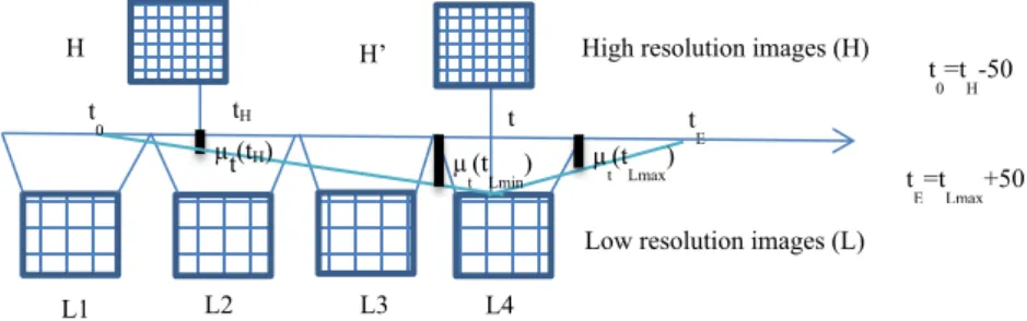
temporal validities of the signal in H and L at the desired time instant t and thus can define the contributions of the corresponding image H and L to the synthetic image H’ that we want to compute. The situation is depicted in Figure 1 where at timestamp t we generate a fused image by combining the two images L4 and H1 since these are the closest in time to t.
Figure 1. Two time series of High and Low resolution images are depicted, with distinct timestamps and temporal density. In black the membership degrees defining the time validity of the images with respect to timestamp t.
Once one has set the range of the temporal domain in which it makes sense to select the images to fuse: i.e., tO and tE, the validity of a timestamp tH can be
computed as follows:
o If t0 tH < t then 𝜇 (𝑡 ) = (𝑡 − 𝑡 ) (𝑡 − 𝑡 )⁄
o If t tH < tE then 𝜇 (𝑡 ) = (𝑡 − 𝑡 ) (𝑡 − 𝑡 )⁄ (1)
We can also compute the validity degree of a low resolution image L at an instant of time t by computing its membership degrees t(tLmin) and t(tLmax)
by applying equation (1) and then taking the greatest validity degree, i.e., we take the best validity of the two extremes of the time range of L:
t(tL)=max( t(tLmin), t(tLmax)), (2)
We then select from the two series the H image and the L image with greatest validities in their series.
A fusion function that satisfies the above stated property is the following: Given two time series <H> and <L> and a desired timestamp t we first
select the input images to fuse H <H> and L <L> such that: Low resolution images (L)
L1 L2 L3 L4 t E H’ H 1
High resolution images (H) t tH µt(tH) µ t(tLmin) µ t(tLmax) t 0 t 0=tH-50 t E=tLmax+50
5 H =argMaxH <H>( t(tH1),…, t(tHm)) and L =argMaxL <L>( t(tL1),…, t(tLm))
Then, for each pixel values l L and h H we compute the Weighted Average:
ℎ = 𝑊𝐴(ℎ, 𝑙) = ( ( ))∗( ( )) ( ( ))∗( ( )) (3) where f(
.
) [0,1]. f is a function associated with a linguistic modifier such asvery, fair, more or less, idem etc, i.e., a concentrator or dilator of its argument.
It is generally defined as f(
.
)=(.
)x with x>1, in case of concentrator, while x<1in case of dilator. The choice of x must be tuned based on sensitivity analysis exploiting training data, i.e., by comparing the correlation obtained between the resulting image H’ and the expected image E at timestamp t, a target image that we have for timestamp t.
In the case the expert knows the dynamics of represented objects; f can be defined by a membership function describing the temporal validity of an image taken in a given period.
Notice that equation (3) can be easily generalized to fuse K input images, provided that their temporal validities are computed by applying equation (1) to their timestamps and that they are selected from the two time series based on the following:
H=argMax_KH <H>( t(tH1),…, t(tHm)), L=argMax_KL <L>( t(tL1),…, t(tLm)) (4)
where argMax_K selects the H which has the validity degree t(tH) within
the K greatest ranked values.
Notice that, fusing more than two images to generate a simulated image can be useful to cope with the very frequent problem of clouds masking the scene in the original images of the time series.
2.2. Soft fusion based on temporal validity and preference (WP)
Let us assume that we know that one of the two time series is better than the other one with respect to the signal in the images, either because it is less affected by noise or because it has undergone preprocessing steps that have cleansed it.
In this case, besides the temporal validity, we want to model in the fusion a preference for one of the two series. Assuming that <H> is preferred to <L> we can formalize the desired properties with the following rule: o if t(tH) is very high then H’ is determined mostly by H and marginally
by L, else it’s a weighted average of H and L with contributions directly proportional to their temporal validities.
very high can be quantified by a positive integer p, a numeric preference
indicating how many times H is preferred with respect to L. mostly and
6 and H depending on p, so that the validity of L is decreased while the validity of H is increased.
We also want not to overestimate the pixel values.
A fusion function that satisfies the above stated properties is the following: given two pixel values l and h for L and H respectively:
ℎ = 𝑊𝑃(ℎ, 𝑙) = 𝑚𝑖𝑛
𝑚𝑎𝑥 𝑊𝐴(ℎ, 𝑙), (𝑡 ) ,
( ) ∗ ( ) /∗ ( ) ( ) /
, 𝑝 ≥ 1 (5)
In which WA(h,l) is defined as in equation (3). While WA is symmetric WP is an asymmetric function. The asymmetry of WP function depends on both the fact that p>1, and the satisfaction of the condition WA(h,l)> t(tH). We can
observe that when (𝑡 ) = 1, the preferred value h has a greater chance to contribute to h’, and its contribution increases with the preference p, unless when p=1 in which case we get exactly the Weighted Average based solely on temporal validities of H and L: h’=min(1, WA(h,l)) . When WA(h,l)> t(tH)
and p>1 we get the minimum between the Weighted Average and the Weighted Preferences.
A dual function satisfying the following properties can be defined: Assuming that <H> is preferred to <L>:
o if t(tH) is very high then H’ is determined mostly by H and marginally by
L, else it’s a weighted average of H and L with contributions directly proportional to their temporal validities.
We also want not to underestimate the pixel values The corresponding function is the following:
ℎ = 𝑊𝑃(𝑙, ℎ) = 𝑚𝑎𝑥
𝑚𝑖𝑛 𝑊𝐴(ℎ, 𝑙), 1 − (𝑡 )) ,
( ) ∗ ( ) /∗ ( ) ( ) /
, 𝑝 ≥ 1 (6)
We can observe that when( (𝑡 )) tends to 1, the preferred value h has a greater chance to contribute to h’ and its contribution increases with p. On the contrary we obtain the weighted average based solely on the temporal validities of H and L.
For the application of this method, some conditions have to be defined for choosing between equation 5 and equation 6. In our experiments we wanted to identify if the input images correspond to a growing or senescent season. In the case of a growing season we do not want to underestimate the NDVI values so we can choose equation 6. Contrarily, in the senescent season we do not want to overestimate so equation 5 must be applied. The identification of the season was made automatically from the timestamps of the images and the tendency of the average NDVI in the time interval between the input images. The method was applied as follows:
7 Senescent season: If tH <t < tL and h H h/(n*m) > l L l/(n*m) or
if tL <t < tH and l L l/(n*m) > h H h/(n*m) then apply equation WP(h,l) (5)
Growing season: If tH <t < tL and h H h/(n*m) < l L l/(n*m) or
if tL <t < tH and l L l/(n*m) < h H h/(n*m) then apply equation WP(l,h) (6)
where n*m is the total number of pixels . This method could be applied differently by changing the conditions for applying equation 5 or 6 and also by selecting a value of p lower than 1 if we wanted to give preference to the low resolution image.
2.4 Soft Fusion considering the temporal validity and the change (WS) The previous soft fusions do not consider the change of the pixel values, i.e., |h-l| while this would be desirable when one wants to enhance edges of change. They typically correspond to those regions where there is a high increase or decrease of the pixel values.
The change can be defined by a positive value as follows: s= min [(| h – l | - smin ) / ( smax p% - smin ), smax]
where smin and smax are the minimum and maximum |h – l| among all pixels in
H and L and smax %p is the maximum |h – l| for %p percentile in H and L.
The desired property is the following:
The more s is high and the more H is valid ( µt(tH) is high) then the more
h’ should be close to h
A simple soft fusion function satisfying the above properties is the following:
ℎ = 𝑊𝑆(ℎ, 𝑙) =(( )∗ ( )∗)∗ ( ) ∗ (∗ ( )∗) (7)
3. Application of the methods to real data
3.1. Data
A short temporal series of high and low resolution images was available for a zone of Brazil for the year 2004. As low resolution images we used the MODIS product MOD13Q1 which provides NDVI composite images each 16 days at 250m spatial resolution. As high resolution images we had CBERS (China-Brazil Earth Resources Satellite) images with 20 m spatial resolution. MODIS images were available at dates 225, 241, 257 and 273 (starting date of the 16-day period). CBERS images were available for dates 228, 254 and 280. The CBERS images were radiometrically normalized to the MODIS ones as described in [6]. Also, several images of a zone of Italy were available for the year 2012. As low resolution images we had one image (date 209) of the MODIS product MOD09Q1 which provides composite images of 8 days at 250m spatial resolution. As high resolution we had two Landsat images (with 30m spatial resolution) in the dates 197 and 213.
8 3.2. Results and quality evaluation
The soft operators defined in section 2 were applied to different temporal combinations of the available images.
The simulated images with the different methods (Weighted Average: WA, Weighted with Preference: WP, and Weighted with Slope: WS) were then compared to the ‘target’ (high resolution image in the date we pretend to simulate) and the following quality indices were computed: correlation, RMSE (Root Mean Square Error) and the accuracy between the simulated and the target image, defined as follows:
𝐴𝑐𝑐𝑢𝑟𝑎𝑐𝑦 = 1 −∑ |ℎ′ − 𝑡 | 𝑛 ∗ 𝑚
in which h’i and ti are the pixel values corresponding to the simulated and the
target images respectively, and n*m is the total number of pixels.
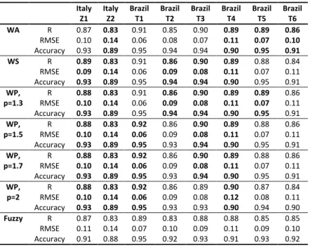
The different temporal combinations for analyzing the proposed methods are shown in Table 1. In Table 2 we show the results obtained with the previous methods in the different temporal combinations of the available images. Analyzing the correlations we observe that the fuzzy rule-based method using three rules equally distributed leads to significantly lower correlations than the different proposed methods using soft operators. When analyzing the proposed methods we observe that in the cases where the input and target images are far away (cases of Brazil T5 and T6: a difference of 52 days) the method leading to the higher correlations is the WA. In the other cases with closer dates (Brazil T1, T2 and T3: difference of 26 days) the results are not so clear, low differences are observed between the different methods using soft operators. Only in the case of the input high resolution date being lower than the target (case T4: -26 days) we observe a better correlation when using the method WP with preference p=2. Conversely, in Italy’s zones the WA leads to lower correlations than the other soft operators, while the WS and WP with p=2 lead to the higher correlations. However we keep observing lower values when using the fuzzy rule-based method in Italy Z1. Regarding the RMSE we observe generally higher errors when using the fuzzy rule-based method (6 out of the 8 cases). In the methods using soft operators we observe that in the further images (cases of Brazil T5 and T6) we obtain again the lower errors when using the WA. In the other cases the best method is difficult to identify, the WA would be clearly selected in cases Brazil T2 and T3. In the other cases there are other methods with similar results to the WA. We observe in 5 out of the 6 cases of Brazil that the WP with p=2 leads to the higher errors, while in Italy’s zone 1 this method together with the WS lead to the lowest values of RMSE. In Italy’s zone 2 there are no significant differences between the soft operators. The Italian zone 2 covers a very dense urban area and thus the setting of the time validity is probably not very appropriate for this scene.
9
Table 1. Temporal combinations used for applying the methods. Timestamps are expressed as day of the year. Hr corresponds to the high resolution image used in the fusion algorithm, Lrmin
and Lrmax are the minimum and maximum timestamps of the composite MODIS image, Target
is the image to simulate, and Dist(t) is the difference in days between the timestamps of the high resolution input image and the Target image.
Italy Z1 Italy Z2 Brazil T1 Brazil T2 Brazil T3 Brazil T4 Brazil T5 Brazil T6
Hr 197 197 254 228 228 254 228 280
Lrmin 209 209 273 241 257 225 273 225
Lrmax 216 216 288 256 272 240 288 240
Target 213 213 280 254 254 228 280 228
Dist(t) 16 16 26 26 26 -26 52 -52
Table 2. Results of the soft fusion methods obtained in the different temporal combinations.
High values of both R and Accuracy and low values of RMSE as associated with good quality of the simulated image with respect to the target image. The best quality indicators triples (R, RMSE, Accuracy) for each simulated image are reported in bold cases.
Italy Z1 Italy Z2 Brazil T1 Brazil T2 Brazil T3 Brazil T4 Brazil T5 Brazil T6 WA R 0.87 0.83 0.91 0.85 0.90 0.89 0.89 0.86 RMSE 0.10 0.14 0.06 0.08 0.07 0.11 0.07 0.10 Accuracy 0.93 0.89 0.95 0.94 0.94 0.90 0.95 0.91 WS R 0.89 0.83 0.91 0.86 0.90 0.89 0.88 0.84 RMSE 0.09 0.14 0.06 0.09 0.08 0.11 0.07 0.11 Accuracy 0.93 0.89 0.95 0.94 0.94 0.90 0.95 0.91 WP, p=1.3 R 0.88 0.83 0.91 0.86 0.90 0.89 0.89 0.86 RMSE 0.10 0.14 0.06 0.09 0.08 0.11 0.07 0.11 Accuracy 0.93 0.89 0.95 0.94 0.94 0.90 0.95 0.91 WP, p=1.5 R 0.88 0.83 0.92 0.86 0.90 0.89 0.88 0.86 RMSE 0.10 0.14 0.06 0.09 0.08 0.11 0.07 0.11 Accuracy 0.93 0.89 0.95 0.93 0.94 0.90 0.95 0.91 WP, p=1.7 R 0.88 0.83 0.92 0.86 0.90 0.89 0.88 0.86 RMSE 0.10 0.14 0.06 0.09 0.08 0.11 0.07 0.11 Accuracy 0.93 0.89 0.95 0.93 0.94 0.90 0.95 0.91 WP, p=2 R 0.88 0.83 0.92 0.86 0.89 0.90 0.87 0.84 RMSE 0.10 0.14 0.06 0.09 0.08 0.12 0.08 0.11 Accuracy 0.93 0.89 0.95 0.93 0.93 0.90 0.94 0.90 Fuzzy R 0.87 0.83 0.89 0.83 0.88 0.88 0.85 0.85 RMSE 0.11 0.14 0.07 0.10 0.09 0.11 0.09 0.10 Accuracy 0.91 0.88 0.95 0.92 0.93 0.91 0.93 0.92 In terms of accuracy, the fuzzy rule-based methods leads to similar results as the RMSE, showing the lower accuracies in 6 out of the 8 cases (the same having higher RMSE values) and the higher accuracies in the other two cases. The WP with p=2 leads generally to lower accuracies, and the WA leads to high accuracies in the Brazil zone. In Italy’s zones 1 we obtain higher accuracies with the WS and the WP with p=2, while in zone 2 all the methods lead to similar results. We can conclude that the WA is the one showing the better compromise between correlation, RMSE and accuracy in the different temporal combinations of the Brazil’s zone. However if we want to use the
10 fused images for edge detection it is not so important having high accuracy but it is important having a high correlation, so we could use the method WP with p=2 in the case of close images. In Italy’s zone 1 the methods WS and WP with p=2 are the best ones in terms of correlation, RMSE and accuracy, while in zone 2 all the methods lead to similar results.
4 Conclusions
The paper proposes some soft fusion operators to generate synthetized images at desired timestamps having two input heterogeneous time series of remote sensing data. The proposed operators were applied to different combinations of input and target images. A fuzzy rule-based fusion method was also applied to the same combinations of images. The validation of the results obtained with the different operators as well as the comparison with the fuzzy rule-based fusion method were analysed in terms of correlation between the simulated and target images, RMSE and accuracy. The proposed fuzzy operators led to higher correlations than the fuzzy rule-based method applied in all the cases and to higher (lower) values of accuracy (RMSE) in most of the cases. These results show how the application of simple soft operators taking into account the time validity of input images and in some cases a preference for the high resolution input image can be used for simulating images with high accuracy and correlation at desired timestamps within the timestamps of the input images.
References
1. Goshtasby, A.A., Nikolov, S.: Guest editorial: Image fusion: Advances in the state of the art. Inf Fusion. 8, 114–118 (2007).
2. Pohl, C., Van Genderen, J.L.: Review article Multisensor image fusion in remote sensing: Concepts, methods and applications. Int. J. Remote Sens. 19, 823–854 (1998).
3. Dammavalam, S.R.: Quality Assessment of Pixel-Level ImageFusion Using Fuzzy Logic. Int. J. Soft Comput. 3, 11–23 (2012).
4. Zhao, L., Xu, B., Tang, W., Chen, Z.: A Pixel-Level Multisensor Image Fusion Algorithm Based on Fuzzy Logic. In: Wang, L. and Jin, Y. (eds.) Fuzzy Systems and Knowledge Discovery. pp. 717–720. Springer Berlin Heidelberg (2005).
5. Yager, R.R.: A framework for multi-source data fusion. Soft Comput. Data Min. 163, 175–200 (2004).
6. Le Maire, G., Marsden, C., Verhoef, W., Ponzoni, F.J., Lo Seen, D., Bégué, A., Stape, J.-L., Nouvellon, Y.: Leaf area index estimation with MODIS reflectance time series and model inversion during full rotations of Eucalyptus plantations. Remote Sens. Environ. 115, 586–599 (2011).
View publication stats View publication stats