Anomalous transport through porous and fractured media

Anomalous Transport through Porous and Fractured

Media

by

Peter Kyungchul Kang

B.S., Seoul National University (2008)

S.M., Massachusetts Institute of Technology (2010)

Submitted to the Department of Civil and Environmental Engineering

in partial fulfillment of the requirements for the degree of

Doctor of Philosophy in the Field of Hydrology

at the

JUN

1 3 201t

MASSACHUSETTS INSTITUTE OF TECHNOLOGY

LIBRARIES

June 2014

©

2014 Massachusetts Institute of Technology. All rights reserved.

Signature redacted

Department of Civil and Environmental Engineering

May 12, 2014

Signature redacted

C ertified by ...

Ruben Juanes

Associate Professor of Civil and Environmental Engineering

Thesis Supervisor

Signature redacted

A ccepted by...,... .. . ...

Heidi M. Nepf

Chair, Departmental Committee for Graduate Students

Anomalous Transport through Porous and Fractured Media

by

Peter Kyungchul Kang

Submitted to the Department of Civil and Environmental Engineering on May 12, 2014, in partial fulfillment of the

requirements for the degree of

Doctor of Philosophy in the Field of Hydrology

Abstract

Anomalous transport, understood as the nonlinear scaling with time of the mean square displacement of transported particles, is observed in many physical processes, including contaminant transport through porous and fractured geologic media, animal and human foraging patterns, tracer diffusion in biological systems, and transport in complex networks. Understanding the origin of anomalous transport is essential, because it determines the likelihood of high-impact, low-probability events and therefore exerts a dominant control over the predictability of a system. The origin of anomalous transport, however, remains a matter of debate.

In this thesis, we first investigate the pore-scale origin of anomalous transport through sandstone. From high-resolution (micron-scale) 3D numerical flow and transport simula-tion, we find that transport at the pore scale is markedly anomalous. We demonstrate that this anomalous behavior originates from the intermittent structure of the velocity field at the pore scale, which in turn emanates from the interplay between velocity heterogeneity and velocity correlation. Finally, we propose a continuous time random walk (CTRW) model that honors this intermittent structure at the pore scale and captures the anomalous

3D transport behavior at the macroscale.

To show the generality of our finding, we study transport through lattice networks with quenched disorder. We again observe anomalous transport originating from the interplay between velocity heterogeneity and velocity correlation. We extend the developed CTRW model to capture the full multidimensional particle transport dynamics for a broad range of network heterogeneities and for both advection- and diffusion-dominated flow regimes.

We then study anomalous transport through fractured rock at the field-scale. We show that the interplay between heterogeneity and correlation in controlling anomalous trans-port can be quantified by combining convergent and push-pull tracer tests because flow re-versibility is strongly dependent on correlation, whereas late-time scaling of breakthrough curves is mainly controlled by velocity heterogeneity. Our transport model captures the anomalous behavior in the breakthrough curves for both push-pull and convergent flow ge-ometries, with the same set of parameters. Moreover, the inferred flow correlation length shows qualitative agreement with geophysical measurements. Thus, the proposed corre-lated CTRW modeling approach furnishes a simple yet powerful framework for character-izing the impact of flow correlation and heterogeneity on transport in porous and fractured media.

Finally, we propose a joint flow-seismic inversion methodology for characterizing frac-tured reservoirs. Traditionally, seismic interpretation of subsurface structures is performed without any account of flow behavior. With the proposed methodology, we reduce the un-certainty by integrating dynamic flow measurements into the seismic interpretation, and improve the predictability of reservoir models by this joint use of seismic and flow data. This work opens up many possibilities of combining geophysical and flow information for

improving subsurface characterization. Thesis Supervisor: Ruben Juanes

Acknowledgments

I am deeply grateful to my family, friends, colleagues, and mentors who helped me to grow

in various ways during my PhD studies. To name only a few, I offer my thanks

to the DOE Office of Science Graduate Fellowship (DOE SCGF) program for supporting my graduate studies for three years;

to the Martin Family Society of Fellows for Sustainability at MIT for support-ing my graduate studies;

to my advisor, Ruben Juanes, for his guidance, mentorship, and support through-out my PhD studies;

to my research mentor, Marco Dentz, who taught me from the basics and helped me to become an independent researcher;

to my thesis committee, Dennis B. McLaughlin and Daniel H. Rothman for their guidance and support towards my studies;

to Tanguy Le Borgne, who provided field experiment facilities and mentored me throughout the field experiments in Ploemeur, France;

to Martin J. Blunt, who shared poscale experiment data and guided my re-search on pore-scale transport;

to Susan Murcott, who inspired me with her works in drinking water issues in developing countries and motivated me to visit Tanzania;

to the members of the Juanes Research Group for their friendship and bound-less enthusiasm for science;

to my parents, In-Sik and Jeung-Hee, and my sister, Sarah, for their uncondi-tional love and support;

and, to my fiancee, SunMin Hwang, for her trust and love towards me. With her love and support, I could finish my PhD thesis with full of joy.

Contents

1 Introduction 25

1.1 Anomalous transport: the breakdown of Fick's law . . . 25

1.2 Numerical experiments on 3D real rock . . . 27

1.3 Anomalous transport through lattice fracture networks . . . 28

1.4 Field experiment on fractured granite . . . 29

1.5 Joint flow-seismic inversion for characterizing fractured reservoirs . . . 30

1.6 Conclusions and future work . . . 31

2 Numerical experiments on 3D real rock 33 2.1 B ackground . . . 33

2.2 Fluid flow and particle tracking through Berea sandstone . . . 35

2.3 Non-Fickian spreading and intermittency . . . 40

2.4 Lagrangian velocity correlation structure and origin of anomalous transport 41 2.5 Continuous time random walk model . . . 44

2.6 Impact of particle injection rule: flux weighted injection vs volume injection 48 2.7 Effective correlated CTRW . . . 51

2.8 D iscussion . . . . 53

3 Anomalous transport through lattice fracture networks 55 3.1 B ackground . . . 55

3.2 Random Lattice Network . . . 57

3.3 Average Transport Behavior . . . 61

3.5 3.6 3.7 3.8

Continuous Time Random Walk Model. . . . M odel Prediction . . . . CTRW model with effective parameterization D iscussion . . . .

. . . 7 2

. . . 74

. . . 77

. . . 7 8 4 Field experiment on fractured granite 4.1 Background . . . . 4.2 Field experiments . . . . 4.2.1 Field site and tracer-test setup . . . . 4.2.2 Field test results . . . . 4.3 Existing models of transport . . . . 4.3.1 Advection-dispersion equation (ADE) model . . . . 4.3.2 Stochastic convective stream tube (SCST) model . . . . . 4.3.3 Multirate mass transfer (MRMT) model . . . . 4.3.4 Comparison of ADE, SCST and MRMT models . . . . . 4.4 Continuous time random walks (CTRW) with correlated velocities 4.4.1 Model formulation . . . . 4.4.2 Limiting cases . . . . 4.4.3 Model implementation . . . . 4.5 Model behavior and field application . . . . 4.5.1 Model behavior . . . . 4.5.2 Field application . . . . 4.6 Summary and Conclusions . . . . 5 Joint flow-seismic inversion for characterizing fractured reservoirs 5.1 Background . . . . 5.2 Overall framework . . . . 5.3 Fluid flow and elastic deformation on rough-walled fractures . . . 5.4 Seismic inversion on orthogonal discrete fracture networks . . . . 5.5 Error model for the compliance field . . . . 5.6 Flow and transport model . . . . 81 . . . . . 81 . . . . . 83 . . . . . 83 . . . . . 85 . . . . . 86 . . . . . 87 . . . . . 89 . . . . . 9 1 . . . . . 93 . . . . . 95 . .. . 96 . .. . 98 . .. . 99 . . . . .103 . . .. . 103 . . . . .107 . . . . .108 113 . . .. . 115 . . ... 120 ... 120 . . .. . 123

5.7 Unifying flow and seismic measurements: least squares . . . 123

5.8 Joint inversion results . . . 125

5.9 Conclusions . . . 125

6 Conclusions and future work 129

6.1 Intellectual contributions . . . 129

6.2 Future work: laboratory experiments using microfluidics . . . 130

List of Figures

1-1 Illustration of the manifestations of anomalous transport. (a) After a point injection of tracers (red star), anomalous transport often shows a strongly non-Gaussian concentration field as opposed to a Gaussian concentration field for Fickian dispersion. (b) Tracer concentration measured from the

fixed control plane shows early time breakthrough and long tailing for

anomalous transport. (c) Time evolution of mean square displacements shows nonlinear increase in time for anomalous transport. . . . . 26

1-2 (a) Three-dimensional normalized velocity magnitude (JvJ/V) through a Berea sandstone sample of size 1.66 mm (approximately 8 pore lengths) on

each side; blue and cyan solid lines indicate two particle trajectories. The domain is discretized into 3003 voxels with resolution 5.55 Pm

(approx-imately 0.03 pore lengths). (b) Velocity autocorrelation function shows

power-law decay of Lagrangian velocity in time. Inset: transition time

dis-tribution shows broad disdis-tribution following truncated power-law. . . . . . 28

1-3 Particle distribution at a fixed time after injection at the origin (red star). . . 29

1-4 (a) Satellite image of the Ploemeur field site where we conducted

field-scale tracer transport experiment through fractured granite (modified from

Google Earth). Inset: map showing the location of Ploemeur, France. (b) Schematic of the convergent tracer tests conducted. (c) Schematic of the

2-1 Areal porosity variation along the longitudinal direction. Areal porosity varies between 0.15 and 0.23. Volumetric porosity of the 3D sample rock is

0.18. Insets: 2D porosity maps at three different locations. White indicates

pore space and black indicates solid rock. . . . 35

2-2 (a) Three-dimensional normalized velocity magnitude (JvJ/V) through a Berea sandstone sample of size 1.66 mm (approximately 8 pore lengths) on each side; blue and cyan solid lines indicate two particle trajectories. The domain is discretized into 3003 voxels with resolution 5.55 Pm (ap-proximately 0.03 pore lengths). (b) Cross section of the Berea sandstone at

rescaled distance (, = 4.16, showing the pore space (white) and solid

grains (black). The average porosity (fraction of void space in the sample) is approximately 18.25%. (c) Cross section of the velocity magnitude at rescaled distance (. = 4.16 (warm colors correspond to higher velocities), illustrating the presence of preferential flow paths. . . . 37

2-3 (a) Average velocity along longitudinal direction. From the incompress-ibility, x-directional mean velocity stays constant. Transverse (y, z) direc-tional velocity has fluctuations around 0 velocity. (b) Probability density functions for Eulerian velocities in each direction. For all directions, we can observe very broad distribution of velocities (more than ten orders of magnitude). Inset: Probability density functions for Lagrangian velocities in each direction. The slope is 0.75 which is steeper than the slope for Eulerian velocity distribution. . . . 38

2-4 (a) Time evolution of Lagrangian mean velocity. Longitudinal Lagrangian velocity follows power 0.2 and in transverse directions Lagrangian mean velocity converges to 0. (b) Time evolution of Lagrangian velocity vari-ance. Both longitudinal and transverse direction exhibits power law decay with respective power 0.1 and 0.2. . . . 39

2-5 (a) and (b) Time series of the normalized Lagrangian velocity and accel-eration, respectively, for the blue particle trajectory in Fig. 2-2(a). The Lagrangian statistics exhibit strongly intermittent behavior in both longitu-dinal and transverse directions. . . . 39

2-6 Time evolution of the centered second spatial moments from particle-tracking

simulation. In the x-direction, particle dispersion is superdiffusive with

slope - 1.5, and in the y and z directions, dispersion is subdiffusive with

slope ~ 0.8. . . . 4 1

2-7 (a) Probability density distributions of the normalized Lagrangian velocity

increments in x, y and z directions, for a time lag T = TA/4. Velocity

increments are normalized with respect to their standard deviation Uoi, Z

X, y, z. (b) Change in probability distributions for different time lags. The

tailing decreases as the time lag increase, but the distribution is still non Gaussian even for the lag time of 4TA. . . . . 42

2-8 (a) Longitudinal Lagrangian velocity autocorrelation,

x,

multiple t values. We can observe the fluctuation of velocity autocorre-lation functions with respect to the average autocorreautocorre-lation function, <

xV, (t, t + r) >t , due to the nonstationarity of the Lagrangian statistics.

(b) Transverse Lagrangian velocity autocorrelation (green),

xv,

2-9 (a) Time evolution of the centered second spatial moments in the

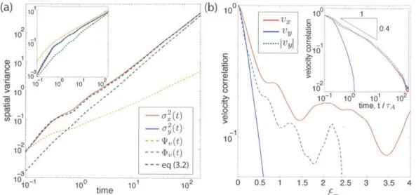
longi-tudinal direction from particle tracking simulation (solid line), prediction from eq (2.3) (black dotted line), and estimations from velocity heterogene-ity alone (T, (t), orange dotted line) and velocheterogene-ity correlation alone ((D, (t), green dotted line). The orange and green lines are shifted along the y axis for clarity. Inset: Time evolution of the centered second spatial moments in the transverse direction. (b) Longitudinal (x, red) and transverse (y, blue) Lagrangian velocity autocorrelation as a function of space along the longi-tudinal direction. All functions are short-ranged. Inset: Longilongi-tudinal (red) and transverse (blue) Lagrangian velocity autocorrelation as a function of

time. Note the strong, long range, correlation of the longitudinal velocity vx and the absolute value of the transverse velocity, IvyI. . . . . 44

2-10 (a,b,c) Longitudinal (x) transition matrix with N = 100 velocity classes for different values of the space transition Ax/A,. The velocity correlation decreases as the sampling distance Ax increases. (d,e,f) Transverse (y) transition matrix with N = 100 velocity classes for different Ay values. We assign 50 bins for positive velocity and another 50 for negative veloc-ity. The z-directional transition matrix is almost identical to y-directional transition m atrix. . . . 46 2-11 (a) Time evolution of the centered second spatial moments from

particle-tracking simulation (solid line) and the prediction with correlated CTRW (dotted line). Inset: Time evolution of the mean particle pair distance. We do not see the exponential increase in the particle pair distance up to

1 0 0

TA. Therefore, chaotic advection is not the mechanism for anomalous

transport. (b)Longitudinal projection of the particle density distribution at fixed times (t = TA, 5TA and IOTA) from direct pore-scale simulation

(solid line), and the correlated CTRW model prediction (dotted line). Inset: Transverse projection of the particle density distribution at fixed times (t = 2_{TA and}

IOTA) from direct simulation (solid line) and the respective CTRW

2-12 (a) Comparison of Lagrangian velocity probability density functions at ev-ery ta for volume injection and flux weighted injection. We can clearly observe the Lagrangian statistics for flux weighted injection case is nonsta-tionary. (b) Comparison of probability density functions of x-directional Lagrangian velocities sampled equidistance in time for volume injection and flux weighted injection . . . 49

2-13 (a) Time evolution of Lagrangian mean velocity for volume injection case.

Mean velocity is approximately constant over time. (b) Time evolution of Lagrangian velocity variance. Both longitudinal and transverse direction

shows no dependence in time. . . . 49

2-14 MSD for two different injection rules. We can observe clear difference between the two cases. . . . . 50

2-15 Velocity autocorrelation for the two different injection rules. Volume

in-jection case shows stronger correlation for both longitudinal and transverse directions. . . . 51

2-16 (a) Time evolution of the centered second spatial moments from particle

tracking simulation (solid line), and predictions from eq (2.6) (black dotted line). (b) Time evolution of the centered second spatial moments from particle-tracking simulation (solid line) and the prediction with correlated CTRW (black dotted line). . . . 52

2-17 Transition matrices for uniform injection case. In time, velocities are very

strongly correlated for small velocities due to the particles in stagnation zones. We have symmetric transition matrix in space. . . . 52

2-18 (a) Probability density distribution of particle transition times. Transition

times sampled at equidistance in time and equidistance in space gives dra-matic difference in the probability distribution. To apply CTRW theory, the proper transition time distribution is the one with volume injection and sampled equidistance in space. (b) Time evolution of the centered second spatial moments from particle tracking simulation (solid line), and predic-tions using effective correlated CTRW (black dotted line). inset: measured transition matrix and simplified transition matrix. . . . . 54

3-1 (a) Schematic of the homogeneous lattice network considered here, with two sets of links with orientation ±a = ±r/4 and spacing I = 1. Boundary

conditions are imposed to realize liner flow geometry. (b) Schematic of the heterogeneous lattice network. . . . 58

3-2 _{(a) Pressure field for log-normal conductivity distribution with variance 0,} (b) Pressure field for log-normal conductivity distribution with variance 1

(c) Pressure field for log-normal conductivity distribution with variance 5. . 58

3-3 Schematic for the two different mixing rules when the two incoming links and the two outgoing links have same fluxes. (a) Complete mixing rule. (b) Streamline routing rule. . . . 60

3-4 (a) Schematic of the lattice network considered here, with two sets of links with orientation ±o = ±7r/4 and spacing I = 1. (b) Particle distribution at nodes (represented by circles of different sizes) at t = 30 for a single realization after injection at the origin at t = 0. . . . . 60

3-5 Particle distribution at fixed time after injection at the origin (red star). In low heterogeneity, transverse spreading significantly increases for plete mixing. Spreading is similar between streamtube routing and com-plete mixing for high heterogeneity. . . . 62

3-6 Time evolution of second spatial moments for complete mixing (solid line)

and streamline routing (dashed line). (a) Longitudinal spreading with con-ductivity variance 0.1. (b) Transverse spreading with concon-ductivity vari-ance 0.1. (c) Longitudinal spreading with conductivity varivari-ance 1. (d) Transverse spreading with conductivity variance 1. inset: Change in the time evolution of transverse spreading for complete mixing with increasing variance. (e) Longitudinal spreading with conductivity variance 5. inset: Change in the time evolution of longitudinal spreading for complete mix-ing with increasmix-ing variance. (f) Transverse spreadmix-ing with conductivity variance 5. inset: Change in the time evolution of transverse spreading for streamline routing with increasing variance. . . . . 64

3-7 Probability density of particle breakthrough position in transverse direc-tion. (a) Comparison between the two different mixing rules for conductiv-ity variance 0.1. (b) Comparison between the two different mixing rules for conductivity variance 1. (c) Comparison between the two different mixing rules for conductivity variance 5. . . . 65

3-8 Particle first passage time distributions for three different conductivity

het-erogeneities and different mixing rules. . . . 65

3-9 Illustration of velocity transition matrix for 2D lattice networks.

Transi-tion matrix considers all 16 possible transiTransi-tions to capture the full particle transport dynam ics. . . . 67

3-10 Velocity transition matrix with equiprobable binning for a-2 = 0.1 and

complete mixing rule. Only four transitions that have forward movement in longitudinal direction are possible out of sixteen possible transitions. Also, note that the probability for each possible transition is almost identical. 67

3-11 Velocity transition matrix with equiprobable binning for a 2 = 0.1 and

streamline routing rule. Only four transitions that have forward movement in longitudinal direction are possible out of sixteen possible transitions. Also, note that the probability for up-down and down-up forward transi-tions have significantly higher probabilities compared to up-up and down-down forward transitions. . . . 68

3-12 Velocity transition matrix with log-scale binning for a 2 = 0.1 and

com-plete m ixing rule. . . . 68

3-13 Velocity transition matrix with log-scale binning for a 2, l = 0.1 and

stream-line routing rule . . . 69 3-14 Velocity transition matrix with equiprobable binning for or2 = 5 and

com-plete mixing rule. Due to strong heterogeneity, 12 out of 16 possible transi-tions are happening. Also, note that up-up and down-down transitransi-tions have triangular m atrices. . . . 69

3-15 Velocity transition matrix with equiprobable binning for a 2 = 5 and

streamline routing rule. Since strong heterogeneity determines the parti-cle transition, there is no noticeable difference between complete mixing and streamline routing. . . . 70

3-16 Velocity transition matrix with log-scale binning for 2 = 5 and complete

m ixing rule. . . . 70

3-17 Velocity transition matrix with log-scale binning for a 2 = 5 and

stream-line routing rule . . . 71

3-18 (a) Aggregate transition matrix for N = 100 velocity classes distributed

with logarithmic scale. (b) Transition probabilities after m = 5 steps from direct Monte Carlo computation (blue solid line) and calculated from the Markov assumption (green symbols). Shown are probability densities for two initial velocity classes: a low velocity class (j = 5, o), and a high velocity class (j = 90, *). Inset: probability of returning to the same initial velocity class as a function of the number of steps for a high initial velocity (class

j

3-19 Comparison between time evolution of MSDs for Monte Carlo simulations

and model predictions. The developed correlated CTRW model is able to accurately capture time evolution of MSDs for all of the conductivity heterogeneities and mixing rules. (a) or. = 0.1 and complete mixing rule. (b) or, = 1 and complete mixing rule. (c) a k = 5 and complete

mixing rule. (d) a'2ik 0.1 and streamline routing rule. (e) (T2ik 1 and streamline routing rule. (f) a 2= 5 and streamline routing rule. . . . . 75

3-20 Probability distributions of transverse particle breakthrough position for

Monte Carlo simulations and model predictions. (a) a2, = 0.1. (b) a 2_

1. (c) a 2.= 5. ... ... 75

3-21 Comparison of FPT distributions of Monte Carlo simulations and model

predictions. . . . 76

3-22 Contour plot of the mean particle density at t = 5 x 102, computed from

direct Monte Carlo simulation (blue solid line), correlated CTRW model (green solid line), and uncorrelated CTRW model (red solid line). . . . 76

3-23 (a) Time evolution of the longitudinal MSD. Inset: Transverse MSD. (b)

Cumulative FPT distribution. . . . 77

3-24 (a) Velocity autocorrelation function for g2 = 1 and a 2 = 5. For

both cases, we can accurately fit exponential correlation function with A =

31. (b) Probability distribution functions of transition time in longitudinal

direction. (c) Comparison between the MSD from MC simulations and CTRW model. Our effectively parameterized CTRW can accurately pre-dict the time evolution of MSDs. Without correlation, we underestimate

M SD (green line). . . . 78

4-1 (a) Satellite image of the Ploemeur field site (modified from Google Earth). Inset: map showing the location of Ploemeur, France. (b) Outcrop of frac-tured granite at the Ploemeur field site. (c) Photo from the installation of double packer system in B I borehole. . . . 84

4-2 Schematic of the tracer tests conducted. (a,b,c) Convergent test with tracer placement at borehole B 1 and pumping from borehole B2. Two different fracture planes at different depths (B 1-2 and B 1-4) are used for two sepa-rate tests. (d,e,f) Push-pull test from borehole B 1. The same two fracture planes (B 1-2 and B 1-4) are used. . . . 85

4-3 Measured breakthrough curves (BTC) for the tracer tests we conducted, in the form of a normalized time (peak arrival at dimensionless time of 1) and normalized concentration (such that the area under the BTC is identi-cally equal to 1). (a) BTCs for fracture plane B 1-2. (b) BTCs for fracture plane B 1-4. . . . 87

4-4 Comparison of the breakthrough curves (BTC) for the MRMT and SCST models characterized by the distributions (4.21) and (4.22) with

#

To = 0.005 and ko = 200, respectively. The BTCs for the convergent and

push-pull scenarios are almost identical in the MRMT approach because solute spreading is irreversible. In contrast, the BTC for the convergent and push-pull scenarios in the SCST model are drastically different: in the absence of local dispersion, the BTC in the push-pull scenario is a delta distribution due to the perfect velocity correlation within each streamtube, i.e., full reversibility. . . . 94

4-5 Key transport characteristics of our proposed CTRW model. (a) O(T) fol-lows the truncated Pareto distribution (4.40). The slope of the power law,

0, characterizes the flow heterogeneity of the fractured medium. As 0

de-creases, the flow heterogeneity increases. (b) Number n, of correlation steps given by (4.35) as a function of parameter a for N = 100 velocity

classes. By changing the value of the diagonal, a, we can systematically vary the strength of the velocity correlation from the uniform transition ma-trix that is equivalent to the uncorrelated velocity field to the identity mama-trix that represents a fully correlated velocity field. . . . 100

4-6 Sensitivity analysis for the peak arrival time on the three parameters of our CTRW model. (a) Change in peak arrival times for a = 0.3 with varying A. Different curves represent different degrees of velocity heterogeneity (3 = 0.5, 0.6, 0.8, 1, 1.2, 1.4). (b) Change in peak arrival times for A = 0.2 with

varying a. Different curves represent different 3 0.5, 0.6, 0.8, 1, 1.2, 1.4.. 104

4-7 Impact of parameters a,

/

/

0.75 and A = 0.2. Middle (c,d): impact of velocity heterogeneity

(/3

0.5, 0.75, 1,1.5, 2) for fixed value of a = 0.03 and A = 0.2. Bottom (e,f):

impact of velocity correlation (A = 0.05, 0.1, 0.3, 0.5, oc) for fixed value of a = 0.03 and 0 = 0.75. . . . 106

4-8 Plot of the mean square error (MSE) between modeled and measured BTCs for different model parameters. The error is for the combined differences of the convergent and push-pull tests. (a) MSE for the B 1-2 fracture with a value a = 0.03. The global minimum is for a = 0.03,

/

minimum is for a = 0.02,

/

4-9 Comparison of measured and modeled BTCs for both convergent and push-pull tests, modeled with the same set of parameters. (a) B 1-2 fracture; model parameters a = 0.03,

/3

/

5-1 Overall framework for joint flow-seismic inversion. The above framework shows how seismic and flow models are integrated to better characterize fractured reservoirs. . . . . 116

5-2 (a) Top fracture surface where the horizontal and vertical length is L = 80 m and fracture aperture maps (void space between the top and bottom

surface) for three different 0 values. For this work, we choose Df = 2.5

for fractal dimension, k, = 10 for the normalized critical frequency and

of = 0.02 for standard deviation of surface heights. (b) Power spectral density for three different 0 values. Change in power spectral density is smoother as we increase 0. Inset: correlation function (-) for different 0 values. . . . 118

5-3 (a) True compliance field of the orthogonal discrete fracture networks that we study. Each link has length equal to 80m and has a compliance value between 10-10 and 10-' m/Pa. (b) Functional relation between fracture compliance and permeability obtained from simulation of fluid flow and elastic deformation on rough-walled fractures for three different 0 values. We parametrize the functional relation with a set of parameters a using the polynomial curve fitting to the data in loglog space: log(bhydraulic) = allog(CT)2 + a2log(CT) + a3. Color of solid circles indicate the pressure

values at each point. We can observe that the pressure values between the compliance of 10-10 and 10-9 m/Pa are around 30 MPa. . . . 121

5-4 (a) True compliance field for the orthogonal discrete fracture network,

in-terpolated to show the smoothed compliance field (CT). (b) Modeled com-pliance field from double beam seismic model (Cm). Note that the modeled compliance field has to be re-scaled to have same mean value with the true compliance filed. (c) Difference between true compliance field (CT) and re-scaled seismic interpreted compliance field (C'm). We find a strong spa-tial correlation between the error (e'c) and the true compliance field (CT).

(d) Error (CT - C'm) with respect to centered CT (CT - (C'A)). We

ob-serve that C'm is compressed compared to CT, and there is a linear relation

5-5 (a) First flow scenario used in estimation. Quarter five-spot flow geometry

with a single injection well (green circle) and a single production well (blue circle). There are four observation wells (red circle) that measures borehole pressure. (b) Second flow scenario used in estimation. A single injection well (green circle) at the left center and a single production well (blue cir-cle) at the right center. (c) Flow scenario used to test the predictability of estimated permeability field. Quarter five-spot flow geometry in different diagonal direction compared with first flow scenario. Predictive scenario is not used in the estimation step. . . . 124

5-6 (a) Difference between the true compliance field (CT) and the corrected

seismically-interpreted compliance field (C"A), which shows that the

cor-rected compliance error (e", = CT - C"l) is small and virtually

in-dependent of the true compliance field CT. (b) Estimated compliance-permeability relationship from joint flow-seismic inversion (blue line) ac-curately captures the true compliance-permeability relationship (red line); the green line is the initial input for our least square procedure. (c) Tracer production curves before (green solid line) and after inversion (blue solid line) compared with the measurements (red solid line). The dashed lines show the performance of the model in predictive mode, in which the model is used after inversion to predict the flow response for a different well con-figuration (a quarter-five spot with injector in the upper-left and producer in the lower-right corner). . . . 126

Chapter 1

Introduction

1.1

Anomalous transport: the breakdown of Fick's law

Understanding flow and transport through subsurface is essential for improving forecasts, management, and risk assessment of many underground technologies, including geologic nuclear waste disposal [17], geologic CO2 storage [137]; oil and gas production from

frac-tured reservoirs [84], enhanced geothermal systems [118], shale-gas development [31, 30], and groundwater contamination and remediation [58, 69]. Since subsurface consists of rock which is highly porous and often fractured, the prediction of flow and transport through sub-surface requires understanding of flow and transport through porous and fractured media.

The transport of mass through porous media is traditionally described with two pro-cesses: advection and dispersion where advection is the translation of the mass following the mean flow direction and the dispersion describes the spreading of the mass. Since Adolf E. Fick introduced the diffusion equation (Fick's law) in 1855 [54], Fick's law still is the dominant framework that describes dispersive transport processes in porous materials, nuclear materials, pharmaceuticals, population dynamics, neurons, semiconductor doping process, etc. Implicit in Fick's law is that the time evo-lution of the mean square

displace-ment (MSD) of passive tracers increases linearly with time, MSD - t. However, the

generality of Fick's law has been questioned since 1926 when L. F Richardson observed how particles disperse in the atmosphere [122]. Again in 1948, Richardson studied the relative displacements of pairs of submersed floats over a fixed interval of time on the west

(c)

y1

3

mean flow direction 0

-010 -b)- Fickian Ca ---- Anomalous 2 10 E 10 - 3 - -- -- -2 10 100 time _time

Figure 1-1: Illustration of the manifestations of anomalous transport. (a) After a point injection of tracers (red star), anomalous transport often shows a strongly non-Gaussian concentration field as opposed to a Gaussian concentration field for Fickian dispersion. (b) Tracer concentration measured from the fixed control plane shows early time breakthrough and long tailing for anomalous transport. (c) Time evolution of mean square displacements shows nonlinear increase in time for anomalous transport.

coast of Scotland and observed the clear breakdown of Fick's law, MSD ~ P a 1 [123]. Since then, anomalous (non-Fickian) transport has been widely observed in many do-mains: transport in amorphous semiconductors, contaminant transport through porous and fractured geologic media, animal foraging, human travel, and diffusion of passive tracers in turbulent flows, to name just a few. The signatures of anomalous behavior are non-Gaussian or multipeaked plume shapes, early breakthrough, long tailing of the first pas-sage time distribution, and nonlinear scaling of the MSD-effects that cannot be captured

by a traditional advection-dispersion formulation [Fig. 1-1]. Understanding the origin of

the slow-decaying tails in probability density is essential, because they determine the like-lihood of high-impact, low-probability events and therefore exert a dominant control over the predictability of a system.

The focus of this thesis is anomalous transport through porous and fractured media. Despite the broad relevance of flow and transport through geologic porous media, our un-derstanding still faces significant challenges due to the almost ubiquitous observation of anomalous transport behavior, from laboratory experiments in packed beds [76, 108], sand

columns [95] and real rock samples [130, 14] to field-scale experiments [56, 88]. Different

mathematical models have been proposed to reproduce anomalous transport by replicating the broad (power-law) distribution of velocity; these include multirate mass transfer [63], fractional advection-dispersion [102], and continuous time random walk (CTRW) mod-els [10, 12].

In this thesis, we investigate the origin of anomalous transport through porous and frac-tured media, and propose a parsimonious stochastic transport model capable of capturing anomalous transport. We first identify the origin of anomalous transport in 3D porous rock using high-resolution 3D numerical flow and transport simulation at the pore scale. To show the generality of our finding, we then extend our model to Darcy-scale transport through lattice networks. We then apply the developed model to study field-scale

anoma-lous transport through fractured geologic media. Finally, we propose a joint flow-seismic

inversion methodology for characterizing fractured reservoirs.

1.2 Numerical experiments on 3D real rock

In the first part of this thesis (Chapter 2), we study the origin of non-Fickian particle trans-port in 3D porous media by simulating fluid flow in the intricate pore space of real rock. We simulate Stokes flow at the same resolution as the 3D micro-CT image of the rock sample, and simulate particle transport along the streamlines of the velocity field [Fig. 1-2(a)]. We find that transport at the pore scale is markedly anomalous: longitudinal spreading is su-perdiffusive, while transverse spreading is subdiffusive. We demonstrate that this anoma-lous behavior originates from the intermittent structure of the velocity field at the pore scale, which in turn emanates from the interplay between velocity heterogeneity and veloc-ity correlation [Fig. 1-2(b)]. Finally, we propose a continuous time random walk model that honors this intermittent structure at the pore scale and captures the anomalous 3D transport behavior at the macroscale. These results have been submitted for publication [80].

(a) (b) 10 10 10 - 10 0 1110to 1 10 - tastintm 10 10 10 1o2

Figure 1-2: (a) Three-dimensional normalized velocity magnitude (IvI/-V) through a Berea sandstone sample of size 1.66 mm (approximately 8 pore lengths) on each side; blue and

cyan solid lines indicate two particle trajectories. The domain is discretized into 3003 vox_

els with resolution 5.55 pum (approximately 0.03 pore lengths). (b) Velocity autocorrelation function shows power-law decay of Lagrangian velocity in time. Inset: transition time dis-tribution shows broad disdis-tribution following truncated power-law.

1.3 Anomalous transport through lattice fracture networks

In the second part of this thesis (Chapter 3), we extend our findings to transport through lattice fracture networks. Flow through lattice networks with quenched disorder exhibits strong correlation in the velocity field, even if the link transmissivities are uncorrelated. This feature, which is a consequence of the divergence-free constraint, induces anomalous transport of passive particles carried by the flow. We show that, for lattice fracture net-works, the interplay between this strong velocity correlation and velocity heterogeneity is again the origin of anomalous transport. We extend the developed CTRW model to cap-ture the full multidimensional particle transport dynamics for a broad range of network heterogeneities and for both advection- and diffusion-dominated flow regimes. The model captures the anomalous longitudinal and transverse spreading, and the tail of the mean first passage time observed in the Monte Carlo simulations of particle transport. We show that reproducing these fundamental aspects of transport in disordered systems requires honor-ing both the correlation and the heterogeneity in the Lagrangian velocity. These results

mean flow direction

Figure 1-3: Particle distribution at a fixed time after injection at the origin (red star).

have been published in Physical Review Letters and Physical Review E [78, 77].

1.4 Field experiment on fractured granite

In the third part of this thesis (Chapter 4), we study anomalous transport through frac-tured rock at the field scale [Fig. 1-4(a)]. Quantitative modeling of flow and transport through fractured geological media is challenging due to the inaccessibility of the under-lying medium properties and the complex interplay between heterogeneity and small-scale transport processes such as heterogeneous advection, matrix diffusion, hydrodynamic dis-persion, and adsorption. This complex interplay leads to anomalous (non-Fickian) transport behavior, and we show that the interplay between heterogeneity and correlation in control-ling anomalous transport can be quantified by combining convergent and push-pull tracer tests because flow reversibility is strongly dependent on correlation, whereas late-time scal-ing of breakthrough curves is mainly controlled by velocity heterogeneity [Fig. 1-4(b)(c)]. In the framework of the developed CTRW model, flow heterogeneity and flow correlation are quantified by a Markov process of particle transition times that is characterized by a dis-tribution function and a transition probability. Our transport model captures the anomalous

(a)(b)

B1

B2

(c) B1 B2

FRANCE\ Ploemelur\

Figure 1-4: (a) Satellite image of the Ploemeur field site where we conducted field-scale tracer transport experiment through fractured granite (modified from Google Earth). Inset: map showing the location of Ploemeur, France. (b) Schematic of the convergent tracer tests conducted. (c) Schematic of the push-pull tracer tests conducted.

behavior in the breakthrough curves for both push-pull and convergent flow geometries, with the same set of parameters. Thus, the proposed correlated CTRW modeling approach furnishes a simple yet powerful framework for characterizing the impact of flow correlation and heterogeneity on transport in fractured media. These results have been submitted for publication [81].

1.5

Joint flow-seismic inversion for characterizing

frac-tured reservoirs

In the fourth part of this thesis (Chapter 5), we propose a joint flow-seismic inversion methodology for characterizing fractured reservoirs. Traditionally, seismic interpretation

of subsurface structures is performed without any account of flow behavior. Here, we present a methodology to characterize fractured geologic reservoirs by integrating flow and seismic data. The key element of the proposed approach is the identification of the intimate relation between acoustic and flow responses of a fractured reservoir through fracture com-pliance. By means of synthetic models, we show that: (1) owing to the strong (but highly uncertain) dependence of fracture permeability on fracture compliance, the modeled flow response in a fractured reservoir is highly sensitive to the geophysical interpretation; and (2) by incorporating flow data (well pressures and production curves) into the inversion workflow, we can simultaneously reduce the error in the seismic interpretation and im-prove predictions of the reservoir flow dynamics. These results have been published in a conference paper and in preparation for journal publication [79].

1.6

Conclusions and future work

In the last chapter of this thesis (Chapter 6), we conclude by summarizing the intellec-tual contributions of this thesis to understanding anomalous transport through porous and fractured media, and we discuss possible future work that could build on this thesis.

Chapter 2

Numerical experiments on 3D real rock

In this Chapter, we first investigate the pore-scale origin of anomalous transport through sandstone. From high-resolution 3D numerical simulation on real 3D rock, we rigor-ously identify the physical origin of observed anomalous transport and develop a predictive stochastic model.

2.1

Background

Fluid flow and transport in porous media is critical to many natural and engineered pro-cesses, including sustainable exploitation of groundwater resources [66, 60], seawater in-trusion into coastal aquifers [53], enhanced oil recovery [114], geologic carbon seques-tration [71, 137], geologic nuclear waste disposal [154], water filseques-tration and membrane technology [131], and drug delivery and chemical signaling through living tissue [50].

Despite the broad relevance of flow and transport through geologic porous media, our understanding still faces significant challenges. One such challenge is the almost ubiq-uitous observation of anomalous (non-Fickian) transport behavior, from laboratory exper-iments in packed beds [76, 108], sand columns [95] and real rock samples [130, 14] to field scale experiments [56, 88]. The signatures of anomalous behavior are early break-through, long tailing of the first passage time distribution, non-Gaussian or multipeaked plume shapes, and nonlinear scaling of the mean square displacement-effects that can-not be captured by a traditional advection-dispersion formulation. Different mathematical

models have been proposed to reproduce anomalous transport, by replicating the broad (power-law) distribution of velocity; these include multirate mass transfer [63], fractional advection-dispersion [102], and continuous time random walk (CTRW) models [10, 12].

In addition to velocity heterogeneity, recent studies have pointed out the importance of velocity correlation in the signature of anomalous transport [90, 39, 78]. In particular, numerical simulations using smoothed particle hydrodynamics of flow and transport on simple 2D porous media suggest that longitudinal spreading is strongly modulated by the intermittent and correlated structure of Lagrangian velocity [35], which is also observed in laboratory experiments in 3D glass bead packs [34]. Moreover, fundamental understanding on the impact of velocity heterogeneity and correlation on transverse spreading is poor. It is known that transverse spreading largely controls overall mixing and, as a result, many chemical and biological processes in natural systems [13, 139, 151, 138, 126].

In this Chapter, we study flow and particle transport through real rock (Berea sand-stone), imaged at the pore scale via micro-computed tomography (micro-CT imaging). We observe strongly non-Fickian spreading behavior in both longitudinal and transverse di-rections, and find complementary anomalous behavior: longitudinal spreading is superdif-fusive, while transverse spreading is subdiffusive. We show that the interplay between pore-scale velocity correlation and velocity heterogeneity is responsible for the observed anomalous behavior. We then develop a stochastic transport model for 3D porous media that incorporates the microscale velocity structure. To show the generality of the proposed framework, we also investigate the impact of particle injection rule on the macroscopic spreading. Finally, we further simplify our stochastic model such that it has only two parameters: one for flow heterogeneity and the other for flow correlation. We show the predictability of the simplified model, and discuss the potential applicability.

0.24 0.22 Z' 0.2 0L) 0

a0.18

Figure 2-1: Areal porosity variation along the longitudinal direction. Areal porosity varies between 0.15 and 0.23. Volumetric porosity of the 3D sample rock is 0.18. Insets: 2D porosity maps at three different locations. White indicates pore space and black indicates solid rock.

2.2

_{Fluid flow and particle tracking through Berea}

sand-stone

We analyze the 3D Lagrangian velocities of a Newtonian fluid flowing through a cube sample of Berea sandstone rock of size L = 1.66 mm on each side. Micro-CT is used to obtain the 3D image of the porous structure at a resolution of 5.55 Am (3003 voxels). Image segmentation identifies each voxel as either solid or void. The characteristic length of the mean pore size is A, ~ 200 gm [109], which is used to define the nondimensional distance

x = _{x/Ac (the sample has ~ 8 characteristic pore lengths in each direction). The porosity}

and pore structure variation along longitudinal direction shows complex porous structure of Berea sandstone [Fig. 2-1].

We simulate Stokes flow (incompressible steady viscous flow) through the pore geom-etry of the Berea sandstone with no-slip boundary conditions at the grain surfaces, using a standard finite volume method [113, 16, 15]. We impose constant pressure boundary conditions at the inlet and outlet faces. The Eulerian velocity field v exhibits a complex structure, with multiple preferential flow channels and stagnation zones [Fig. 2-2(a)]. To confirm the incompressible steady viscous flow, we calculate mean velocity along

longi-tudinal direction [Fig. 2-3(a)]. As expected, x-directional mean velocity stays constant confirming the incompressible steady viscous flow. The transverse velocities fluctuates around 0. If we compute the effective mean velocity (average velocity over pore space), we

obtain V- = 6.37ptm/s, ig = -0.16pm/s, and -- -0.26pm/s. The heterogeneity of the

flow field can be characterized by the probability density function of Eulerian velocity field [Fig. 2-3(b)]. In all directions, Eulerian velocity shows strongly heterogeneous distribution with power -0.5. The overall structure of the probability distribution between longitudi-nal and transverse direction is similar but longitudilongitudi-nal direction has higher probability for larger velocity. 29% of the pore space has velocity larger than the mean velocity (-2) and

71% of the pore space has velocity smaller than the mean velocity (T-). This indicates that there are a few preferential paths and large number of stagnation zones. Probability density function of Lagrangian velocities sampled equidistance in time shows slope -0.75 [Fig. 2-3(b)inset]. This implies higher probability of having small velocities for Lagrangian velocity distribution compared to Eulerian velocity distribution. This is because the parti-cles with small velocities are sampled much more compared to fast velocities if we sample equidistance in time.

To study the transport properties, we simulate the advection of particles along stream-lines of the stationary 3D flow field. We trace streamstream-lines using a semianalytical formula-tion to compute entry and exit posiformula-tions, and transit times, through each voxel traversed by individual streamlines [109]. To initialize the streamlines, we place 104 particles at the inlet face, following a flux-weighted spatial distribution through the pore geometry. To obtain particle trajectories that are long enough to observe macroscopic behavior, we concatenate particle trajectories randomly within the same class of the flux probability distribution (we have confirmed that the flux distribution at inlet and outlet faces are virtually identical). To ensure representative statistics of transverse displacement, we reinject a particle (following the same flux-weighted protocol) whenever its distance to one of the lateral boundaries is less than 2 voxels. We compute the mean Lagrangian velocity across all trajectories, V, and define the characteristic time to travel the average pore size as T_{A = Ac/V, which is used to}

rescale time. Two particle trajectories are shown in Figure 2-2(a).

veloc-(b)

4f

Figure 2-2: (a) Three-dimensional normalized velocity magnitude (IvI/V) through a Berea sandstone sample of size 1.66 mm (approximately 8 pore lengths) on each side; blue and cyan solid lines indicate two particle trajectories. The domain is discretized into 3003 vox_ els with resolution 5.55 pm (approximately 0.03 pore lengths). (b) Cross section of the

Berea sandstone at rescaled distance G = "I = 4.16, showing the pore space (white) and

solid grains (black). The average porosity (fraction of void space in the sample) is approx-imately 18.25%. (c) Cross section of the velocity magnitude at rescaled distance (. = 4.16 (warm colors correspond to higher velocities), illustrating the presence of preferential flow paths.

(a) x1le 12, 10: - V 4 2 2 0 0 -2 -4--0 0 2 3 4 5 6 7 8 (b) ,06 CO *0 2. CL 1 - positive VX 1 4 negative VX 0.5 - positive Vy - negative V 10 2 10 -2 e 0.75 10 o 10 -6 tO6 10 :2 to2 -10 10 10-5 velocity 10

Figure 2-3: (a) Average velocity along longitudinal direction. From the incompressibility, x-directional mean velocity stays constant. Transverse (y, z) directional velocity has fluc-tuations around 0 velocity. (b) Probability density functions for Eulerian velocities in each direction. For all directions, we can observe very broad distribution of velocities (more than ten orders of magnitude). Inset: Probability density functions for Lagrangian veloci-ties in each direction. The slope is 0.75 which is steeper than the slope for Eulerian velocity distribution.

ity variance for ensemble of particles in all directions [Fig. 2-4]. We observe power law decay of Lagrangian velocity mean and variance indicating nonstationarity of Lagrangian statistics. The nonstationarity and the power-law decay originates from the flux-weighted injection and the strongly heterogeneous velocity field. Theflux-weighted injection places large number of particles to high velocity zone, and particles experience heterogeneous velocity field and slowly converges to stationary velocity field.

To further investigate Lagrangian transport behavior, we analyze individual particle tra-jectories. The temporal evolution of the Lagrangian velocity and acceleration for a particle indicate strongly intermittent behavior, both in the longitudinal (x) and the transverse (y, z)

directions of the flow, alternating between long periods of stagnation and bursts of high variability [Fig. 2-5(a)(b)]. Similar intermittent behavior in the longitudinal direction has been observed in a 2D porous medium consisting of a random distribution of disks [35]. In the transverse direction, particles with high positive velocities jump to high negative velocities-an anticorrelation that was also observed in the particle transport through sim-ple lattice networks [78].

(a) 30 -20 10 0) 0 10 -0 0 1 2 a) 1 10 1 1 10 10 E 10-C CV _a__ 0.2: 0)Y C9 ___ 10-1 10 0 10 1 time, t / TA 102 0 (D C ~~ 0. A 2 10~ 100 10 102 time,t /TA

Figure 2-4: (a) Time evolution of Lagrangian mean velocity. Longitudinal Lagrangian velocity follows power 0.2 and in transverse directions Lagrangian mean velocity converges to 0. (b) Time evolution of Lagrangian velocity variance. Both longitudinal and transverse direction exhibits power law decay with respective power 0.1 and 0.2.

3

(a)

[2

(b)

time,tI

Figure 2-5: (a) and (b) Time series of the normalized Lagrangian velocity and acceleration, respectively, for the blue particle trajectory in Fig. 2-2(a). The Lagrangian statistics exhibit strongly intermittent behavior in both longitudinal and transverse directions.

2.3 Non-Fickian spreading and intermittency

To investigate the impact of the observed intermittent behavior of individual particles on the macroscopic spreading of the ensemble of particles, we compute the time evolution of the longitudinal and transverse mean square displacements (MSD) with respect to the center of mass of a point injection, i.e., initializing every particle's starting position to an identical reference point. For the longitudinal direction (x), the MSD is given by o (t)= ((X(t) - (X(t))) 2) where (-) denotes the average over all particles. The same definition

is applied to the transverse directions to compute o2 _{and a}2_{. At early times, longitudinal}

MSD exhibits ballistic scaling, o ~, t2_{, characteristic of perfectly correlated stratified}

flows [141]. After this initial period, the MSD follows a non-Fickian superdiffusive scaling 2 (t) ~ tI'5. The MSD in the transverse directions also scales as 2 , a2 ~ t2 at early

times but, in contrast, then slows down to an asymptotic non-Fickian subdiffusive scaling

Y , o to-8 . (Fig. 2-6).

Our hypothesis is that the observed non-Fickian anomalous spreading is a consequence of the observed intermittent behavior in the Lagrangian velocity. To quantify the intermit-tent behavior, we compute the velocity increment probability density function (PDF). The Lagrangian velocity increment associated to a time lag T is defined as ATv = v(t+T) - v(t)

where v(t) = [X(t + T) - X(t)]/T. The velocity increments are rescaled with respect to

their standard deviation, ATv/ATv. We find that the velocity increment PDFs in both the

longitudinal and transverse directions collapse (Fig. 2-7(a)); an indication that intermit-tent behavior is equally significant in all directions. This multidimensional intermittency originates from the combined effect of the 3D pore structure and the divergence-free con-straint on the velocity field, which results in a misalignment between the local velocity and the mean flow direction. The PDF of the velocity increments is characterized by a sharp peak near zero, and exponential tails. The peak reflects the trapping of particles in stagna-tion zones, while the exponential tails indicate that large velocity jumps are also probable due to the strong heterogeneity in the velocity field-a signature of the observed inter-mittency [35, 34]. As T increases, the slope of tail increases and the peak becomes less

2 x-direction 10 1.5 10 10 00 0.8 -1 y-direction -10 10 2 10 z-direction -3 10 100 101 10 time, t/rA

Figure 2-6: Time evolution of the centered second spatial moments from particle-tracking simulation. In the x-direction, particle dispersion is superdiffusive with slope - 1.5, and in the y and z directions, dispersion is subdiffusive with slope - 0.8.

PDF is still strongly non-Gaussian showing the persistent anomalous nature of the pore scale fluid transport (Fig. 2-7(b)). This non-Gaussian character indicates that pore-scale fluid flow cannot be modeled using the Langevin description with white noise [138].

2.4 Lagrangian velocity correlation structure and origin

of anomalous transport

From velocity increment pdf, we observed signature of flow intermittency as the sharp peak near zero and exponential tails. The peak represents strong flow correlation due to stagnation zones, and exponential tail represents strong velocity fluctuation from heteroge-neous velocity field. Now we formulate the time evolution of second spatial moments as a function of flow correlation and flow heterogeneity to investigate their respective impact on particle spreading.

p (a) A01(b) - - 0 E ) r /1 10 10 "-1 0a) (10 .Z -22 10 20 2 CL 3 a. 10 -04 ₁₀₀ -4' -10 -5 0 5 10 -10 -5 0 5 10 AV/UAv, _{Av/ A,}

Figure 2-7: (a) Probability density distributions of the normalized Lagrangian velocity

increments in x, y and z directions, for a time lag T = rA/4. Velocity increments are

nor-malized with respect to their standard deviation cvi, i = x, y, z. (b) Change in probability

distributions for different time lags. The tailing decreases as the time lag increase, but the distribution is still non Gaussian even for the lag time of 4TA.

Let Xv (T, q) be the velocity autocorrelation between times T and q,

__ ([v(T) - (v(T))][v(q) - (v(r))])

xv(T,) (T) (2.1)

where of(rj) is the variance of the Lagrangian velocity at time T. Velocity autocorrelation functions at different T values in longitudinal and transverse direction (Fig. 2-8) shows long range correlation in longitudinal direction and short range correlation in transverse direction.

From the definition of the MSD [3], we can express MSD as,

or (t) 2 dn c (1) d 'v(T)v(T, 'q). (2.2)

0 0

When the velocity standard deviation, aO(T), follows slow decay in time with respect

to Xv(T, TI) (we confirmed this), the MSD can be approximated as

o (t) : 2 d r (7) dT Xv (T, q). (2.3)