Bounds for the first eigenvalue of the elastically supportedmembrane on convex domains

0044-2275/03/050879-24 DOI 10.1007/s00033-003-3212-3

c

° 2003 Birkh¨auser Verlag, Basel Mathematik und Physik ZAMPZeitschrift f¨ur angewandte

Bounds for the first eigenvalue of the elastically supported

membrane on convex domains

R. Sperb

To Larry Payne on his eightieth birthday

Abstract. Barta’s principle and gradient bounds for the torsion function are the main tools for

deriving lower bounds for the first eigenvalue. The optimal domains are an infinite strip, a disk or an annulus in different situations.

Mathematics Subject Classification (2000). 35P15.

Keywords. Eigenvalues of the Laplacian, Robin boundary conditions.

1. Introduction

   ∆u + λu = 0 in Ω ∂u ∂n+ hu = 0 on ∂Ω (1.1)

is usually called the “elastically supported membrane”. The constant h > 0 plays the role of a spring constant, with h = 0 corresponding to a free boundary and h = ∞ describing a clamped boundary. In applications a probably more important aspect is the connection with diffusion problems with radiation at the boundary. In all cases however a lower bound for the first eigenvalue λ₁(h) is of main interest, and many results have appeared in the literature.

In this paper lower bounds are derived for domains with boundary of positive mean curvature. The method used is an adaption of earlier works of Payne & Philippin [9] and the author [17].

The main idea is to find a good function v in Barta’s principle stating that if v≥ 0 in Ω and

∆v + µv≤ 0 in Ω, ∂v

then λ1≥ µ .

In the choice of the function v the solution of the torsion problem (

∆ψ + 1 = 0 in Ω

ψ = 0 on ∂Ω (1.3)

will play a central role as an auxiliary function. There are other choices of auxiliary problems. The torsion problem has the advantage that many bounds are known for the quantities relevant for the application to problem (1.1). In addition in two dimensions sharper results are known. This is also true if problem (1.1) and (1.3) are considered on a surface, which is equivalent to the “inhomogeneous membrane”

   ∆u + λρ(x)u = 0 in Ω ∂u ∂n+ hm(x)u = 0 on ∂Ω (1.4)

with positive functions ρ(x), m(x) . In this case the torsion problem (1.3) has to be replaced by the Poisson problem

(

∆p + ρ = 0 in Ω

p = 0 on ∂Ω . (1.5)

The lower bounds for λ₁(h) derived in Theorems 3.1, 3.2, 3.3, 5.1 are all con-sequences of Lemma 2.1 in which a bound for |∇ψ|2 or _ρ1|∇p|2 is the basis. Our main concern here are plane domains, but the bound given in Theorem 3.3 is valid in higher dimensions as well. Theorem 3.2 is due to Payne & Philippin [9], who proved it for the fixed membrane (h→ ∞) . Theorem 4.1 was proven by P´olya-Szeg¨o [13] for the fixed membrane. The version for the elastically supported membrane is given in C. Bandle [2]. It is repeated here in order to compare with the different bounds. In Section 6 some numerical values are listed in order to give some idea of how close these bounds may get.

2. Construction of a function v(x)

v(x)

v(x)

The basic construction of a function v(x) for Barta’s principle is first developed. It will be used later on in four different cases.

Let x be a generic point of Ω and set

t(x) = ε(ψm− ψ(x)) , (2.1)

with ε a parameter to be chosen later and ψ the solution of (1.3). We then set s(x) = ε−12 · f(t(x)) , _(2.2)

where the function f can be selected also. From (2.2) it follows that ∇s = −ε12 df

dt · ∇ψ . (2.3)

It is convenient to introduce the (dimensionless) variable

σ = ε12 · s . _(2.4)

It is now assumed that we can write for some A(σ)

∇s = −ε12 · A(σ) · ∇ψ , _(2.5)

so that

∆s = ε12 · A(σ) − ε32 _A0_(σ)· |∇ψ|2_{. (2.6)} Hence the function v(x) = X(s(x)) satisfies

∆v + µv = dX ds ∆s + d2X ds2 · |∇s| 2_{+ µX} = ε12_A· dX ds h 1 + εA 0 A |∇ψ| 2i₊d2X ds2 εA 2_{· |∇ψ|}2_{+ µX .} (2.7)

We further assume that X(s) satisfies d2X

ds2 + a(s) dX

ds + µb(s) X = 0 , (2.8)

where a(s), b(s) will be chosen below. Then the combination of (2.7) and (2.8) yields ∆v + µv = ε12_AdX ds h 1 + ³ εA 0 A − ε 1 2_aA ´ |∇ψ|2i_{+ µX[1− εA}2_{b· |∇ψ|}2_{] . (2.9)}

At this point it is assumed that a gradient bound is known, written in the form

ε|∇ψ|2B(σ)≤ 1 . (2.10)

Then we choose a(σ), b(σ) such that −A0

A + aA = B , (2.11)

bA2= B , (2.12)

which allows to write

∆v + µv ={√ε X0(s) A(σ) + µ X(s)}[1 − εB(σ) |∇ψ|2] . (2.13) By (2.10) the [ ] -term is nonnegative. We now have to ensure that the { } -term is nonpositive. In terms of the variable σ the differential equation (2.8) is with the selection (2.11), (2.12) X00+ ³_A0 A + B A ´ X0+µ ε B A2 X = 0 . (2.14)

This can be written in selfadjoint form as (p(σ)X0)0+µ

ε q(σ) X = 0 , (2.15)

with p(σ) = e(σ) A(σ) , q(σ) =B_Ae(σ) , where e(σ) = exp

³ Z _B A ´

, (2.16)

and the integral is chosen such that e(0) = 0 . In addition to the differential equation (2.15) we select the boundary conditions

X0(0) = 0, X0(σ₀) + h· ε−12 B 1 2

A X(σ0) = 0 , (2.17)

with σ₀= f (εψm) .

We can now prove that the { } -term in (2.13) is nonpositive. To this end consider the function

g(σ) =¡εX0(σ) A(σ) + µ X(σ)¢e(σ) . (2.18) Then g(0) = 0 and

g0(σ) = ε(p· X0)0+ µ(Xe)0

= ε(pX0)0+ µqX + µe(σ)· X0 = µe(σ) X0.

But p(σ)≥ 0 , q(σ) ≥ 0 , so that (2.15) implies immediately that X0≤ 0 if µ is the first eigenvalue of (2.15) with corresponding positive eigenfunction X(σ) .

Hence we have g(σ)≤ 0 , that is

∆v + µv≤ 0 in Ω . (2.19)

To check the boundary inequality of (1.2) we compute (using (2.5) ∂v ∂n+ hv = dX ds · ∂s ∂n+ h· X = dX ds ε 1 2 · A(σ) |∇ψ| + h · X , and by (2.17) we see that

∂v

∂n+ hv = h· X £

1− ε12 · B12 · |∇ψ|¤≥ 0 , _(2.20) where the inequality is again a consequence of (2.10).

We can now summarize as follows

Lemma 2.1. Let ψ be the solution of (1.3) and ψm = maxΩψ(x) . Let ε be

a positive parameter, f (t) a nonnegative function and suppose df_dt = A(σ) with t = ε(ψm− ψ) , σ = f(t) .

Let X(σ) be the first eigenfunction of (p(σ)X0)0+µ ε q(σ) X = 0 in (0, σ0) X0(0) = 0, X0(σ0) + h· ε−12 B 1 2_(σ0) A(σ₀) X(σ0) = 0 , (2.21)

with σ₀ = f (εψm) , p(σ) = e(σ) A(σ) , q(σ) = B_A(σ)_(σ)e(σ) , e(σ) = exp(

R _B

A) ,

e(0) = 0 .

Then the first eigenvalue of (1.1) satisfies λ₁≥ µ1

ε . For later on it is also convenient to state Lemma 2.2. The first eigenvalue µ₁ of

(p(σ) X0)0+ µq(σ)X = 0 in (0, σ0) X0(0) = 0, X0(σ₀) + h· X(σ₀) = 0

is decreasing with increasing length σ₀ of the interval (p > 0, q > 0, h > 0 ). Proof.This is an immediate consequence of Rayleigh’s principle for µ₁: Assume σ₁> σ₀. Then µ₁(σ₁) = inf v Z σ1 0 p· v 0 2_{dσ + h· v}2_(σ 1) Z σ1 0 qv 2_dσ . Choose v(σ) = ( u(σ), 0≤ σ ≤ σ₀ u(σ₀), σ₀< σ≤ σ₁, where u(σ) is the first eigenfunction for (0, σ₀) . Then

µ1(σ1)≤ Z σ0 0 pu 0 2_{dσ + hu}2_(σ 0) Z σ0 0 qu 2_{dσ + u}2_(σ 0) Z σ1 σ0 q dσ ≤ Z σ0 0 pu 0 2_{dσ + hu}2_(σ 0) Z σ0 0 qu 2_dσ = µ1(σ0) .

Remark. In contrast to the eigenvalue λ₁ ≡ λ₁(∞) of the fixed membrane the eigenvalue λ(h) is not a monotone domain functional, i.e. if Ω⊂ bΩ the associated eigenvalues do not necessarily satisfy λ₁(h)≥ bλ₁(h) (see also Payne-Weinberger [11]). A counter-example is given e.g. in Section 6.

3. Applications of Lemma 1

For the first result the starting point is a gradient bound of [14] stating that |∇ψ|2_≤1 ε ¡ 1− exp(−2ε(ψm− ψ)) ¢ , (3.1) with ε = k0

τ , τ = max∂Ω|∇ψ| , curvature of ∂Ω = k ≥ k0. For later applications

it is important to note that one can always take ε = k0

τ , with τ≥ τ .

For k₀→ 0 (3.1) reduces to the bound of Payne [6] |∇ψ|2_{≤ 2(ψ}

m− ψ) . (3.2)

Now, for an interval (−s0, s0) the solution of (1.3) is

ψ(x) = 1 2(s 2 0− x2) so that x = [2(ψm− ψ(x))] 1 2_. This leads to the choice

s(x) = [2(ψm− ψ(x))] 1

2_{. (3.3)}

We now select s(x) appropriate for the bound (3.1) and such that for ε→ 0 it reduces to (3.3). Such a choice is

s(x) = ε−12£_exp¡_2ε(ψm− ψ(x)) − 1¢¤12_{, (3.4)} or in the notation of (2.1)

f (t) = e2t− 1 . (3.5)

Consequently one finds

A(σ) = 1 + σ

2

σ , (3.6)

and the bound (3.1) can be expressed in the form B(σ) = 1 + σ

2

σ2 . (3.7)

A short calculation shows that

e(σ) = σ , (3.8)

p(σ) = 1 + σ2, (3.9)

which means that the eigenvalue problem (2.21) is now ( ((1 + σ2)X0)0+µ ε X = 0 in (0, σ0) X0(0) = 0, X0(σ₀) + hε−12_{(1 + σ}2₀₎−12_{X(σ0) = 0, σ0= [e}2εψm− 1]12_. (3.11) The first result may be stated as

Theorem 3.1. Assume that the curvature k of ∂Ω is bounded below by k₀> 0 and max_Ωψ ≤ ψ_m, max∂Ω|∇ψ| ≤ τ . Set ε = k_τ0 , ν = −1₂ + i(µ_ε −1₄)

1 2, σ₀= [e2εψm− 1]12 . Then

λ₁(h)≥ µ₁(h) where µ₁ is the first positive solution of

−µ· ε− 1 2Im[P_ν−1(i· σ₀)] Re[Pν(iσ0)] = h . (3.12) Pν, Pν−1: Legendre functions.

Remark 3.1. For the quantities ψm and τ one can take upper bounds ψm, τ .

This follows for ψm from Lemma 2.2, for τ it is implied in the derivation of the

bound (3.1).

Remark 3.2. Invariance of (3.11). A question that may arise is whether a different choice of a function f (t) in (3.5) would lead to a different eigenvalue problem, and one could then try to optimize f (t) . This is not the case as the following calculations show.

With the abbreviations t = ε(ψm− ψ) and y = et assume that in the place

of (3.4) we have

s(x) = ε−12 · f−1_(y) for some f . Then

∇s = −ε12 df −1 dy · y · ∇ψ , but df−1 dy = 1 f0(σ), σ = ε 1 2 · s , and therefore A(σ) = f (σ) f0(σ). The gradient bound (3.1) can be written as

B(σ) = 1 1−_y12 = y 2 y2− 1 = f2 f2− 1 .

A short calculation gives the associated differential equation (2.21) of Lemma 2.1 as _³ f f0 p f2− 1 · X0(σ) ´₀ +µ ε f0f p f2− 1 X = 0 . Choosing the new variable z =pf2− 1 one finds again

¡

(1 + z2)X0¢0+µ

ε X = 0 in (0, z0) ,

with z₀=√e2εψm− 1 as in (3.11), and the boundary conditions are the same as

well.

Remark 3.3. The change of variable σ = sinh(√εs) transforms (3.11) into ( X00+√ε tanh(√εs)X0+ µX = 0 in (0, s₀) X0(s0) + hX(s0) = 0 s₀=√1 ε arch(e εψm_{) .} (3.13)

This shows that for ε → 0 one has X(s) = cos(√µs) and s₀ = √2ψm. In

particular one is led to

λ₁≥ π

2

8ψm

as proven by Payne [7] by different means.

The second result is a straightforward extension of an eigenvalue estimate of Payne & Philippin [9] to the case of the elastically supported membrane. It is based on their gradient bound

|∇ψ|2_{≤ ε(ψ} m− ψ) (3.14) where now ε = 1 + ³ 1−2M0 ψm ´1 2 , (3.15) with M0= min ∂Ω (k· |∇ψ| 3_{) (3.16)}

for a convex domain. In the case of an ellipse of semiaxes a, b one has M₀= a4b4

(a2+ b2)3 and

ε = 1 +|a2− b2| a2+ b2 .

It follows from another gradient bound of Payne & Philippin [8] that one may take M₀= k0

k3_m, 0 < k0≤ k ≤ km. (3.17) The important point is that with the choice (3.17) the equality sign holds in (3.14) if Ω is a disk or an infinite strip.

Choosing now s(x) =pε(ψm− ψ(x)) (3.18) one is led to p(s) = ε 2· s 2 ε−1_{, q(s) =} 2 ε s 2 ε−1

so that Lemma 2.1 leads to the eigenvalue problem      (s2ε−1· X0)0+ 4 ε2 · s 2 ε−1· µX = 0 in (0, s₀₎ X0(0) = 0, X0(s₀) +2 εh· X(s0) = 0, s0= p εψm. (3.19)

In terms of the stretched variable σ =2_εs the solution of the differential equation is X(σ) = σν· J−ν(√µσ) , J = Bessel function, ν = 1− 1_ε and the boundary condition at σ₀=

q

4ψm

ε becomes

X0(σ₀) + h· X(σ₀) = 0 . Note that the function σν· J−ν(σ) has the series expansion

∞ X k=0 (−1)k k! Γ(k + 1− ν) ³_σ 2 ´2k .

Collecting now all facts and using identities for Bessel functions we may sum up in

Theorem 3.2. Assume that the curvature k of ∂Ω satisfies 0 < k₀≤ k ≤ km.

Set ε = 1 + s 1− k0 4ψ_m· k3_m, ν = 1− 1 ε, σ0= s 4ψm ε . Then λ₁(h)≥ µ₁(h) , where µ₁(h) is the first positive solution of

√

µ J1−ν( √

µσ0)

J_−ν(√µσ₀) = h . (3.20)

Remark 3.4. The invariance property again holds for (3.19): one could choose in the place of (3.18) s(x) = f [ε(ψm− ψ(x))] , f arbitrary, and Lemma 2.1 will

again lead to (3.19).

Remark 3.5. An extension of the famous Faber-Krahn inequality for λ₁(= λ₁(∞) ) to the case of the elastically supported membrane was proven by Bossel [3]:

One has λ₁(h)≥ µ₁(h) where µ₁(h) is the solution of √ µ J₁ ³q µA π ´ J₀ ³q µA π ´ = h, A = |Ω| . (3.21)

A comparison of the bounds given by (3.20) or (3.21) is given in Section 6.

3.2. Domain Ω_ΩΩ⊂ R_{⊂ R⊂ R}NNN_{, N, N, N≥ 2≥ 2≥ 2}

Although the main interest is in plane domains, a result valid in higher dimensions as well is added here. The gradient bound in the present case is [14]

|∇ψ|2_{≤ 2(ψ} m− ψ) αψ + 1 αψm+ 1 , (3.22) with α = (N− 1)H0 τ , H = mean curvature of ∂Ω≥ H0> 0 .

Here it is again important for applications that one may take an upper bound τ for τ . We set ε = α 2(1 + αψm) , (3.23) and r(x) = α(ψm− ψ(x)) αψ(x) + 1 . (3.24) We now define s(x) = ε−12 · (r(x))12_{. (3.25)} One finds then

∇r = −2ε(1 + r)2_{∇ψ (3.26)} and ∇s = −ε12 ∇r 2r12 =−ε 1 2 (1 + r) 2 r12 ∇ψ . (3.27)

Setting σ = ε12 · s we thus have in the notation of Lemma 2.1 A(σ) =(1 + σ

2₎2

σ , B(σ) =

(1 + σ2)2

which means that the eigenvalue problem (2.21) now takes the form    ((1 + σ2)2X0)0+µ εX = 0 in (0, σ0) X0(0) = 0, (1 + σ2₀) X0(σ₀) + hε−12 · X(σ₀) = 0 , with σ0= (αψm) 1 2_. (3.29)

The solution of (3.29) can be written in terms of Legendre functions Pm ν .

Theorem 3.3. Assume that the mean curvature H of ∂Ω satisfies H≥ H₀> 0 . Set α = (N−1)H0

τ , ε = α

2(1+αψm) where τ , ψm are upper bounds for the

respective quantities. Then one has

λ₁(h)≥ µ₁(h)

where µ₁(h) is the first positive solution of √ ε(1 + ν)Im P ν 0(iσ0) Re Pν 1(iσ0) = h (3.30) with ν =p1 + µ_ε, σ₀= q α ψ_m.

Remark 3.6. Equation (3.30) is obtained by applying relations for the deriva-tives of Legendre functions (see e.g. [1], p. 334) and using the fact that the first eigenfunction of (3.29) is of the form

X(σ) = (1 + σ2)−12 · P₁ν_{(iσ), ν =} r

1 +µ ε .

Remark 3.7. Lemma 2.2 implies that an upper bound ψ_m for ψm is sufficient.

Remark 3.8. The eigenvalue problem (3.29) is also invariant in the same sense as before.

4. Upper bounds for λ

λ

λ

(h)

(h)

(h)

A. Extension of a bound of P´olya-Szeg¨o

Let Ω be a starshaped plane domain whose representation in polar coordinates (r, ϕ) with respect to some origin is r = R(ϕ) . Set

B = I ∂Ω ds ~r· ~n, ~r = radius vector,|~r| = R(ϕ) , ~ n = exterior normal (4.1)

and let L be the length of ∂Ω , A the area of Ω . The following immediate extension of a classical result of P´olya-Szeg¨o [13] then holds (see also C. Bandle [2], p. 141):

Theorem 4.1. Set α = h_B·L. Then

λ₁(h)≤ µ₁(α)· B

2A (4.2)

where µ₁(α) is the first positive solution of √

µ· J₁(√µ)

J₀(√µ) = α . (4.3)

Equality holds in (4.2) if Ω is a disk.

Proof. For the convenience of the reader we repeat the steps of the proof which are essentially the same as in [13]. According to Rayleigh’s principle one has

λ₁(h)≤ D(v) + h I ∂Ω v2ds Z Ω v2dx , D(v) = Dirichlet’s integral v : trial function . Following P´olya-Szeg¨o we use the trial function

v = g ³ _r

R(ϕ) ´

, where g is any C1 function. Then one has

D(v) = π 2 Z 0 RZ(ϕ) 0 g0 2 ³ ₁ R2(ϕ) + ˙ R2 R4(ϕ) ´ r dr dϕ .

Here we have used a prime for derivative of g with respect to its variable and a dot for dR_dϕ . Choosing the new variable t = _R(ϕ)r the Dirichlet integral becomes

D(v) = 2π Z 0 ³ 1 +R˙ 2 R2 ´ dϕ 1 Z 0 g0 2(t)t dt . An elementary calculation shows that

2π Z 0 ³ 1 +R˙ 2 R2 ´ dϕ = B . Analogously one has

Z Ωv 2_{dx =} 2π Z 0 1 Z 0 g2(t)t dt R2(ϕ)dϕ = 2A 1 Z 0 g2(t)t dt . Rayleigh’s principle then tells us that

λ₁(h)≤ B 1 Z 0 g0 2(t)t dt + h· L · g2(1) 2A 1 Z 0 g2(t)t dt = B 2A 1 Z 0 g0 2(t)t dt + αg2(1) 1 Z 0 g2(t)t dt ,

but the second expression on the right is just the Rayleigh quotient for a radially symmetric solution on the unit circle. The optimal choice is known to be g(t) = J₀(√µt) , where µ solves (4.3).

B. Application of an inequality of Payne & Rayner

It was shown in [10] that the first eigenfunction u₁ in the fixed membrane problem

satisfies _Z Ω u2₁dx≤ λ1 4π ³ Z Ω u₁dx ´2 , (4.4)

with equality if Ω is a disk. As an application of this inequality one finds the following upper bound (see [15]):

λ₁(h)≤ λ1 2(λ₁A− 4π)

©

λ₁A + h· L − [(λ₁A− h · L]2+ 16πh· L]12ª_{. (4.5)} This inequality obtained by taking as a trial function in Rayleigh’s principle v = u₁+ c , applying (4.4) and then optimizing the constant c .

Remark 4.1. In some cases a slightly different version may also be useful: take any function v satisfying v = 0 for which the quantities

d = Z Ω |∇v|2_{dx, n} 2= Z Ω v2dx, n₁= Z Ω v dx can be calculated. Then one finds analogously to (4.5)

λ₁(h)≤ 1 2(n₂A− n2₁) © n₂·L·h+d·A−[(n₂·h·L−d·A)2+ 4d·h·L·n2₁]12ª_{. (4.6)}

5. Inhomogeneous membrane

The torsion problem on a surface S , i.e., e

∆ eψ + 1 = 0 in Ω⊂ S, eψ = 0 on ∂Ω , (5.1) where we have used the notation e∆ for the Laplace-Beltrami operator of a surface, is equivalent to the Poisson problem (1.5). If the line element ds of S satisfies

ds2= ρ(x1, x2)¡(dx1)2+ (dx2)2¢, (5.2) then e ∆u = 1 ρ ³ _∂2_u (∂x1)2 + ∂2u (∂x2)2 ´ = 1 ρ∆u , (5.3)

and the normal derivative _∂∂_en on ∂Ω in S is ∂u ∂en= 1 √ ρ ∂u ∂n. (5.4)

Problem (1.4) can be interpreted as e

∆eu + λeu = 0 in Ω ⊂ S , (5.5)

∂eu

∂en+ h· emeu = 0 on ∂Ω ⊂ S , (5.6) with m(x) =e m√(x)_ρ .

This correspondence between a problem on a surface and an inhomogeneous problem can be exploited in many ways (see e.g. [2], [16]). Later on we will need bounds for the gradient and the solution of the Poisson problem and we list some results of this type in the following.

For problem (5.1) it was shown in [16] that | e∇ eψ|2_≤ 1

K(e

provided that the Gaussian curvature KG of S satisfies

KG≥ K > 0 , (5.8)

and

kg+ K· eτ ≥ 0 on ∂Ω , (5.9)

where kg is the geodesic curvature of ∂Ω⊂ S and

eτ = max

∂Ω | e∇ eψ| = max∂Ω

1 √

ρ |∇ψ| . (5.10)

A sufficient criterion for the validity of (5.9) is

K· A + kg· L ≥ 0 , (5.11)

where A =R_Ωρ dx is the measure of Ω in S and L = H_∂Ω√ρ ds the measure of ∂Ω in S .

Equality holds in (5.7) if Ω is a geodesic strip Sg on a sphere, i.e. the region

represented in spherical coordinates by Sg: n (ϑ, ϕ),π 2 − β < ϑ < π 2 + β, 0≤ ϕ ≤ 2π, 0 < β < π 2 o . (5.12)

For Sg the solution of (5.1) is given by

e

ψ = R2· log ³_{sin ϑ}

cos β ´

, R = radius of the sphere . (5.13) Here of course KG = K = _R12.

Finally we describe the correspondance between problem (5.1) and the geodesic strip Sg. First, the Gaussian curvature is

KG=−

∆(log ρ)

2ρ , (5.14)

and the geodesic curvature becomes kg= 1 √ ρ ³ k +1 2 ∂ ∂n(log ρ) ´ , k = ordinary curvature of ∂Ω . (5.15) Take now Ω as an annulus of radii R₁, R₂ and

ρ = ρ(r) = 1

(1 + γr2)2 . (5.16)

Then KG= 4γ and the solution of (1.5) is

p = 1 4γ log ³_{r(1 + γR}2 1) R1(1 + γr2) ´ , (5.17) with R₁> 0 and R₂= _γR1 1.

One then has ³|∇p|2 ρ + 1 K ´ e2Kp= (1 + γR 2 1)2 16γ2R2₁ = const. , (5.18) and the maximum value is attained for r =√1_γ and becomes

pm= 1 4γ log ³_{1 + γR}2 1 2√γ R₁ ´ = 1 2K log ³ 1 + K·A 2 L2 ´ , (5.19) with A = 2π 1 γR1 Z R1 r dr (1 + γr2)2 = π 1− γ R₁2 γ(1 + γR2₁), (5.20) L = 4π R1 1 + γR2₁. (5.21)

In this case one also finds that K· eτ + kg= K·

A

L+ kg= 1

r(1− γr + |1 − γr|) ≥ 0 . (5.22)

5.2. A lower bound for λλλ₁₁₁(h)(h)(h) for (1.4)

The calculations are completely analogous to the ones leading to Theorem 3.1: one just has to replace ε there by −K . Hence setting now

s(x) = K−12£₁− exp¡− 2K(p_m− p(x))¢¤ 1

2 _{, (5.23)}

where p is the solution of (1.5), and by equivalence, p(x) = eψ(x) . In the notation of Section 2 one thus finds

A(σ) = 1− σ

2

σ , (5.24)

and the bound (5.7) leads to

B(σ) = 1− σ

2

σ2 , (5.25)

and similarly as in Section 3 the eigenvalue problem now is    ((1− σ2)X0)0+ µ KX = 0 in (0, σ0) X0(0) = 0, X0(σ₀) + ehK−12(1− σ2₀)−12X(σ₀) = 0 with σ₀= [1− e−2Kpm]12. (5.26)

One can check that v(x) = X(s(x)) satisfies ∂v

if we choose eh = h· m0, m0= min

∂Ω m(x) .

The solution of (5.26) is given by

X(σ) = Pν(σ)· Qν−1(0) + Qν(σ)· Pν−1(0), ν =− 1 2 + r 1 4 + µ K, (5.28) where P, Q are Legendre functions, and summarizing one is led to

Theorem 5.1. Suppose the following inequalities hold: (a) −∆(log ρ) 2ρ ≥ K > 0 in Ω (b) √1 ρ ³ k +1 2 ∂ ∂n(log ρ) ´ ≥ kg on ∂Ω, k = curvature of ∂Ω . (c) K· A + kg· L ≥ 0, A = Z Ω ρ dx, L = I ∂Ω √ ρ ds .

Set σ₀= (1− exp(−2K p_m)12 , p_m≥ max

Ω p(x) , p(x) = solution of (1.5) and ν =−1 2+ r µ K + 1 4, β = p 1− σ2₀· h m₀ν√K , m0= min∂Ω m(x) .

Let µ₁(h) be the first positive solution of P_ν−1(σ₀) + (β− σ₀)Pν(σ0) Q_ν−1(σ₀) + (β− σ₀)Qν(σ0) =−2 πcot ³_π 2 (ν− 1) ´ . (5.29)

Then the first eigenvalue of (1.4) satisfies

λ₁(h)≥ µ₁(h) , (5.30)

and the equality sign holds if m =√ρ , ρ is given by (5.16) and Ω is an annulus of radii R₁> 0 and R₂= √1_γ, with Robin boundary conditions for r = R₁ and Neumann boundary conditions for r = R₂.

Remark 5.1. The change of variable σ = sin(√K s) transforms (5.26) into    X00−√K· tan(√K s)X0+ µX = 0 in (0, s₀) X0(0) = 0, X0(s₀) + eh· X(s₀) = 0, s₀= √1 K cos −1_(e−K pm_{) .} (5.31)

In this form the limiting case K→ 0 becomes obvious and it is also evident that an upper bound for pm may be used.

Remark 5.2. Bounds for pm were given by C. Bandle [2]: If KG ≤ Km and Km· A < 4π , then pm≤ 1 Km log 4π 4π− KmA . (5.32)

The equality sign holds in (5.32) if Ω is a geodesic circle on a sphere or, equiva-lently, if ρ(r) is given by (5.16) and Ω is a disk. Then one finds

p(r) = 1 4γ log ³_{1 + γR}2 1 + γr2 ´ , R = Radius . (5.33) If KG≥ K > 0 it was shown in [16] that one has

pm≤

1 K log

1

cos( bd√K), (5.34)

where bd is the radius of the largest geodesic circle inscribed in Ω⊂ S . If Ω is an annulus of radii R , _γR1 one finds

pm= 1 K log 1 cos( bd√K)= 1 4γ log ³_{1 + γR}2 2√γ R ´ , (5.35)

so that one has the equality sign in this case.

Using the bound (5.34) one finds that one may take

σ₀= sin( bd√K) (5.36)

in Theorem 5.1. Note that b d≤ max y∈∂Ω ³ min x∈Ω y Z x p ρ(s) ds ´ (5.37) and the integral may be taken over a straight line from x to y .

6. Examples

6.1. A survey of bounds for the torsion function

Let Ω be a plane domain of area A and boundary length L . The torsional rigidity S is defined as S = Z Ω ψ dx = Z Ω |∇ψ|2_{dx ,}

It was shown by P´olya-Szeg¨o [13] that ψm≤

A

4π , (6.1)

with equality for a disk. This inequality was sharpened by Payne [5] who showed that

ψm≤

r S

2π, (6.2)

which is an improvement of (6.1) since the classical Saint-Venant inequality (proven in [13]) states that

S≤ A

2

8π. (6.3)

In (6.2), (6.3) the optimal domain is the circle. A different type of bound was found in [6]: If Ω is convex then

ψm≤

d2

2 , d = inradius of Ω , (6.4) with equality if d is an infinite strip.

If Ω is strictly convex with curvature k≥ k0> 0 then inequality (6.4) can be sharpened. One has (see [16])

ψm≤ τ k₀ log ³ cosh r k₀ τ d ´´ , (6.5)

but one needs an upper bound for τ = max∂Ω|∇ψ| . Bounds for τ will be given

below.

A number of lower bounds for ψm are also known. It was shown by Payne [5]

that one has

ψm≥ 1 4π ³ A−pA2− 8πS ´ , (6.6)

which can be combined with the inequality of P´olya-Szeg¨o [13] S≥ A

2

4B, B defined in (4.1) , (6.7) or the inequality of Payne & Weinberger [12].

S≥A 2 8π h 1− 2ν 1− ν − 2ν2 (1− ν)2 log ν i , ν = 1−4πA L2 . (6.8)

In the last three bounds equality holds again for a disk. A further bound is (see [2])

ψm≥

˙r2

Often one can find good bounds for ψm by exploiting the fact that ψm depends

monotonically on the domain. A bound which becomes sharp in the limit for an infinite strip was also given in [6]: for a convex domain one has

ψm≥

A2

2L2 , (6.10)

and this can be further improved if k₀> 0 . It follows from an inequality of Webb [18] that ψm≥ L− k₀A 2L− 3k₀A· A2 L2 , (6.11)

with equality for a disk or in the limit of an infinite strip.

A bound for τ , the maximum of |∇ψ| was first derived by Payne in [6] who showed that for a convex domain

τ≤ d , (6.12)

with equality for an infinite strip.

If Ω is strictly convex, i.e. k≥ k₀> 0 then Fu & Wheeler [4] proved that τ ≤ d ³ 1−k0d 2 ´ , (6.13)

where the equality sign holds for a disk and an infinite strip. The same is true for the bound of Webb [18]

τ2≤ ψm

2− 3k0τ

1− k₀τ . (6.14)

6.2. Some numerical results

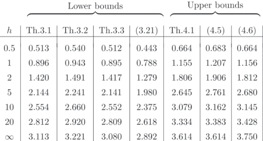
In order to get an idea of how close the bounds for λ₁(h) are let us first look at a case where most quantities needed are easy to get. This is true e.g. if

A. Ω =Ω =Ω = Ellipse of semiaxes (2,1) The quantities needed are:

A = 2π , L = 9.68845 , B =5₂π , k₀= 1₄, ψm= 0.4 , τ = 0.8 .

For (4.6) the function ν(x, y) = 1−x2

4 − y2 was taken. Some bounds for λ1(h)

Lower bounds z }| { z Upper bounds}| { h Th.3.1 Th.3.2 Th.3.3 (3.21) Th.4.1 (4.5) (4.6) 0.5 0.513 0.540 0.512 0.443 0.664 0.683 0.664 1 0.896 0.943 0.895 0.788 1.155 1.207 1.156 2 1.420 1.491 1.417 1.279 1.806 1.906 1.812 5 2.144 2.241 2.141 1.980 2.645 2.761 2.680 10 2.554 2.660 2.552 2.375 3.079 3.162 3.145 20 2.812 2.920 2.809 2.618 3.334 3.383 3.428 ∞ 3.113 3.221 3.080 2.892 3.614 3.614 3.750

Table 1. Bounds for λ₁(h) of an ellipse of semiaxes (2,1) Remarks.

1. The value for λ₁(∞) (determined numerically) is ∼ 3.567 . Note how close to this value the entry 3.614 is, which is the bound j₀2 _2AB of P´olya-Szeg¨o. 2. The value for λ₁(h) of the circumscribed rectangle of sides (4,2) is 1.357 and

this is larger than the value 1.155 found in Theorem 4.1. This is an example showing that λ1(h) does not depend monotonically on the domain.

B. Domain bounded by two arcs y

Γ

1 Ω 1

x Γ

Γ : circular arc of radius 2 and length 2π₃ L = 4π₃ , A = 0.724688 , B = 4π , k₀=1₂

In the following a list of possibilities is given how to get bounds for the required quantities ψm and τ . Inequalities (6.1) and (6.6) combined with (6.7) give

whereas (6.11) yields the cruder lower bound ψm ≥ 0.0157 . Monotonicity with

respect to the circumscribed ellipse of semiaxes a = 1 , b = 2−√3 gives ψm≤ 1 2¡ 1 a2+ 1 b2 ´ = 0.0335 , whereas Payne’s bound (6.4) is

ψm≤ 0.0359 ,

If we combine the best upper bound for ψm with Webb’s inequality (6.14) we find

τ ≤ 0.2494 , whereas Fu & Wheeler’s bound (6.13) yields

τ≤ 0.25 . If the best bound for τ is used in (6.5) one obtains

ψm≤ 0.0351 .

Finally the function v(x, y) = 1 32(4− x 2_{− (y −}√₃₎2_{)(4− x}2_{− (y +}√₃₎2₎ satisfies ∆v =−1 +1 2(x 2_{+ y}2_{) in Ω, v = 0 on ∂Ω ,} and hence ψm> vmax= 1 32= 0.03125 . Also one has

τ >|∇v|max= 0.232 . If v(x, y) is used in Rayleigh’s principle for λ₁ one gets

λ₁≤ 46.56 .

The best bounds for ψm and τ and v(x, y) in (4.6) were used to get the Table

λ₁(h)≥ λ₁(h)≤ z }| { h Th.3.1 Th.3.2 (3.21) Th.4.1 (4.5) (4.6) 0.5 1.91 1.85 1.96 2.75 2.82 2.77 1 3.67 3.55 3.70 5.33 5.51 5.30 2 6.76 6.56 6.63 9.84 10.44 9.74 5 13.59 13.24 12.34 19.75 21.78 19.29 10 20.23 19.81 16.93 29.17 31.91 28.01 20 26.45 26.04 20.43 37.53 39.11 35.49 ∞ 37.02 36.83 25.1 50.14 46.56 46.56

Table 2. Bounds for λ₁(h) C. Oval domain

A slight deformation of a circle given in polar coordinates as r = 1 + 0.2· cos3ϕ

is the last example.

−0.8 −0.4 0 0.4 0.8 1.2 −1 −0.75 −0.5 −0.25 0 0.25 0.5 0.75 1 x y

The relevant quantities are

A = 3.18086 , L = 6.35409 , B = 6.4303 , k₀= 0.3125 , km= 1.25 .

Inequalities (6.1) and (6.6), (6.7) give

and (6.14) then yields

τ < 0.6633 .

In Table 3 we list the numerical results obtained with these bounds. λ₁(h)≥ λ₁(h)≤ z }| { h Th.3.1 Th.3.2 (3.21) Th.4.1 0.5 0.662 0.640 0.879 0.885 1 1.186 1.149 1.565 1.579 2 1.950 1.899 2.536 2.567 5 3.118 3.064 3.919 3.986 10 3.847 3.804 4.697 4.790 20 4.330 4.301 5.177 5.285 ∞ 4.917 4.912 5.712 5.846

References

[1] M. Abramowitz and I. Stegun, Handbook of mathematical functions. Dover, New York, 1970. [2] C. Bandle, Isoperimetric inequalities and applications. Pitman, London, 1980.

[3] M. H. Bossel, Longuers extr´emales et fonctionelles de Domaine. Complex Variables 6 (1986), 203-234.

[4] S. L. Fu and L. T. Wheeler, Stress bounds for bars in torsion. J. Elasticity 3 (1973), 1-13. [5] L. E. Payne, Some isoperimetric inequalities in the torsion problem for multiply connected

regions. Studies in Math. Anal. and Related Topics: essays in honor of G. P´olya, Stanford Univ. Press, 270-280, 1962.

[6] L. E. Payne, Bounds for the maximum stress in the Saint Venant torsion problem. Ind. J. mech. Math. Special issue (1968), 51-59.

[7] L. E. Payne, Bounds for the solutions of a class of quasilinear elliptic boundary value prob-lems in terms of the torsion function. Proc. Royal Soc. Edinburgh 88A (1981), 251-265. [8] L. E. Payne and G. A. Philippin, Some remarks on the problems of elastic torsion and of

torsional creep. Some Aspects of Mechanics of Continua, Part I. Jadavpur University, 32-40, 1977.

[9] L. E. Payne and G. A. Philippin. Isoperimetric inequalities in the torsion and clamped membrane problem for convex plane domains. SIAM J. Math. Analysis 14 (1983), 1154-1162.

[10] L. E. Payne and M. E. Rayner, An isoperimetric inequality for the first eigenfunction in the fixed membrane problem Z. angew. Math. Phys. 23 (1972), 13-15.

[11] L. E. Payne and H. F. Weinberger, Lower bounds for vibration frequencies of elastically supported membranes and plates SIAM J. of Appl. Math. 5 (1957), 171-182.

[12] L. E. Payne and H. F. Weinberger, Some isoperimetric inequalities for membrane frequencies and torsional rigidity. J. Math. Anal. Appl. 2 (1961), 210-216.

[13] G. P´olya and G. Szeg˝o, Isoperimetric inequalities in mathematical physics, Princeton Uni-versity Press, 1952.

[14] P. W. Schaefer and R. Sperb, Maximum principles for some functionals associated with the solution of elliptic boundary value problems. Arch. Rat. Mech. Anal. 61 (1976), 65-76. [15] R. Sperb, Obere und untere Schranken f¨ur den tiefsten Eigenwert des elastisch gest¨utzten

Membran. Z. angew. Math. Phys. 23 (1972), 231-244.

[16] R. Sperb, Maximum principles and their applications. Academic Press, New York, 1981. [17] R. Sperb, Optimal bounds in semilinear elliptic problems with nonlinear boundary

condi-tions. Z. angew. Math. Phys. 44 (1993), 639-653.

[18] J. R. L. Webb, Maximum principles for functionals associated with the solution of semilinear elliptic boundary value problems. Z. angew. Math. Phys. 40 (1989), 330-338.

R. Sperb

Seminar f¨ur Angewandte Mathematik ETH-Zentrum

CH-8092 Z¨urich

e-mail: sperb@sam.math.ethz.ch (Received: June 16, 2003)

To access this journal online:

http://www.birkhauser.ch