Characterization of a building's operation using automation data: a review and case study

Publisher’s version / Version de l'éditeur:

Building and Environment, 118, pp. 196-210, 2017-03-25

READ THESE TERMS AND CONDITIONS CAREFULLY BEFORE USING THIS WEBSITE. https://nrc-publications.canada.ca/eng/copyright

Vous avez des questions? Nous pouvons vous aider. Pour communiquer directement avec un auteur, consultez la première page de la revue dans laquelle son article a été publié afin de trouver ses coordonnées. Si vous n’arrivez pas à les repérer, communiquez avec nous à PublicationsArchive-ArchivesPublications@nrc-cnrc.gc.ca.

Questions? Contact the NRC Publications Archive team at

PublicationsArchive-ArchivesPublications@nrc-cnrc.gc.ca. If you wish to email the authors directly, please see the first page of the publication for their contact information.

NRC Publications Archive

Archives des publications du CNRC

This publication could be one of several versions: author’s original, accepted manuscript or the publisher’s version. / La version de cette publication peut être l’une des suivantes : la version prépublication de l’auteur, la version acceptée du manuscrit ou la version de l’éditeur.

For the publisher’s version, please access the DOI link below./ Pour consulter la version de l’éditeur, utilisez le lien DOI ci-dessous.

https://doi.org/10.1016/j.buildenv.2017.03.035

Access and use of this website and the material on it are subject to the Terms and Conditions set forth at

Characterization of a building's operation using automation data: a

review and case study

Gunay, Burak; Shen, Weiming; Yang, Chunsheng

https://publications-cnrc.canada.ca/fra/droits

L’accès à ce site Web et l’utilisation de son contenu sont assujettis aux conditions présentées dans le site

LISEZ CES CONDITIONS ATTENTIVEMENT AVANT D’UTILISER CE SITE WEB.

NRC Publications Record / Notice d'Archives des publications de CNRC: https://nrc-publications.canada.ca/eng/view/object/?id=38721cdd-c257-4ffb-8353-5a78e71420ea https://publications-cnrc.canada.ca/fra/voir/objet/?id=38721cdd-c257-4ffb-8353-5a78e71420ea

Characterization of a Building’s Operation Using Automation Data: a Review and

Case Study

Burak Gunay1,2, Weiming Shen1, Chunsheng Yang3 1

Construction Portfolio, National Research Council Canada, Ottawa, Canada 2

Civil and Environmental Engineering, Carleton University, Ottawa, Canada 3

Information and Communication Portfolio, National Research Council Canada, Ottawa, Canada Burak.Gunay@carleton.ca; Weiming.Shen; Chunsheng.Yang@nrc-cnrc.gc.ca

Abstract: This paper presents a critical review of the automated on-going commissioning (AOGC)

methods for air-handling units (AHU) and variable air volume terminal (VAV) units in commercial buildings. The common faults studied in the literature were identified. The diagnostic approaches taken and the characteristics of the fault-symptom datasets utilized were categorized. It was found that the diagnostics methods were vastly fragmented, and most of them employed pure-statistical approaches. Only a few studies attempted to assimilate the automation data within the underlying physical processes. In addition, a large fraction of the reviewed literature has been devoted to physical faults in AHUs. Only a few studies were conducted to diagnose faults-related with controls programming and faults at the zone level. Upon the literature survey findings, an inverse greybox modelling-based AOGC approach was put forward. Its strengths and weaknesses were demonstrated through a case study conducted using the archived building automation system (BAS) data of an office building in Ottawa, Canada. The results of this case study indicate that inverse greybox modelling-based AOGC is a promising method to diagnose both physical and controls programming related faults at AHUs and VAVs.

Keywords: Automated on-going commissioning; Fault detection and diagnostics; Inverse modelling;

Greybox modelling; Commercial buildings

1.

Introduction

A survey in 2004 identified that more than 50% of the buildings in the United States with building automation systems (BAS) do not operate per their design intent [1]. Improper operating conditions in building equipment and components are estimated to waste 30 to 50% of the energy use in commercial buildings [2-7]. Given that indoor climate control in commercial buildings in North America accounts for more than 15% of the secondary energy use, over 10% of the CO2 emissions and a major driver for new energy infrastructure, early diagnoses of these improper operating conditions represent great potential to edu e o e ial uildi gs’ e i o e tal a d e o o i i pa t a d to p o ide o fo ta le, healthy, and productive indoor environments [8, 9].

During the service life of a building, some of the sensors and actuators inevitably fail; and parts of the building envelope lose its ability to resist heat, air, and moisture transfer. At least as important as these physical system and component failures, inappropriate operating setpoints and equipment schedules can result in energy waste and/or chronic discomfort conditions. Traditionally, these improper operating

conditions (i.e., faults) remain invisible to the facility managers until the occupants begin to complain or a labour-intensive retro-commissioning is undertaken.

Automated on-going or continuous commissioning (AOGC) is a process to characterize the operation of a

building through a network of sensors [10], and resolve operating problems, improve comfort, and optimize energy use [11]. The operational data from connected sensors and actuators in modern automation and control networks in commercial buildings represent great potential to employ AOGC methods. Particularly, the research conducted during IEA EBC Annexes [12-14] and ASHRAE RPs [15, 16] advanced the state-of-the-art AOGC in buildings. Despite this research potential, AOGC has been seldom employed in commercial buildings [17]. As recently highlighted at the Experts Research Forum on Intelligent Buildings [18], we need scalable AOGC methods that can be used in different types of buildings without manual tuning and any extra configurations.

This paper first presents a critical review of the state-of-the-art AOGC methods in commercial buildings. The scope of the review entails studies on fault detection and diagnostics, prognostics, virtual sensing, remote auditing, and continuous health monitoring efforts on air handling units (AHU) and variable air volume (VAV) terminal units in the last 20 years. The common faults studied in the literature were identified. The diagnostic approaches taken and the characteristics of the fault-symptom datasets utilized were categorized. By looking at the distribution of the studies across these categories, research needs were identified. Subsequently, upon the literature survey findings, an inverse greybox modelling-based AOGC approach was put forward. Its advantages and limitations were demonstrated through a case study conducted using the archived BAS data of an office building in Ottawa, Canada.

Our focus in this paper is on the research conducted to diagnose and triage faults in air-handling units (AHU) and variable air volume (VAV) terminal units. This is due to their common usage in the North American commercial building stock, and due to the fact that the controls infrastructure deployment and programming for these pieces of equipment are custom and manual – and thus prone to human-error. Despite the large number of papers from the literature, fault diagnoses research for the mass-manufactured plant level equipment is outside the scope of this study.

2. Literature review

Identifying improper operating conditions from existing sensor networks in BASs has been vastly studied. In general, the process is executed in three consecutive stages: (1) detect, (2) isolate, and (3) triage the improper operating conditions. The first-stage deals with detecting whether or not there is an a o al i a uildi g’s ope atio . The se o d-stage deals with isolating the sensor, actuator, equipment or controls programming issues causing the detected anomaly in operation. The faults can be grouped as hard-faults – issues in sensors, actuators, equipment – or soft-faults – issues in controls programming [19]. Hard-faults often require component replacement and manual-labour, whereas most soft-faults can be automatically corrected without human intervention (e.g., [20, 21]). The process of detecting and isolating faults in tandem is defined as fault diagnosis. The third-stage deals with proposing an importance ranking of the diagnosed faults in terms of their urgency for health, productivity, comfort, and energy use [22].

Table 1: The AHU and VAV faults studied in the literature.

Component Faults References

AHU cooling and heating coils

Valve stuck open [7, 25-37]

Valve stuck closed [7, 25-31, 33, 34, 36, 38] Valve stuck partially open [7, 25-29, 31, 33, 36, 38-44] Leaky valve [7, 19, 25-27, 29, 31-34, 36, 39, 43,

45, 46]

Unstable valve control [28, 29, 31, 36, 47]

Undersized coil [26, 36]

Coil fouling [26, 29, 33, 36, 40, 43, 46]

AHU dampers Outdoor air intake damper stuck [2, 7, 25-29, 31-33, 35, 36, 38-40, 42, 46, 48-55]

Return air damper stuck [7, 19, 25, 29, 33, 49, 51, 56] Exhaust air damper stuck [7, 27-29, 31, 36, 49]

AHU sensors Supply air temperature bias [7, 19, 25-27, 30, 32, 37, 40, 44, 51, 57-70]

Return air temperature bias [7, 25, 26, 37, 40, 48, 51, 65-67] Mixed air temperature bias [25, 26, 30, 37, 48, 51, 66]

Supply air pressure sensor [27, 35, 36, 49, 51, 52, 57, 60, 64, 65, 67-73]

Other sensors that may be available (CO2, RH) [52, 61, 68]

AHU fans Efficiency degradation [29, 41, 43, 48] Supply or return fan stuck at constant rate [27, 28, 40, 44, 49]

Return fan complete failure [3, 26, 27, 29, 31, 60, 68, 69, 71] Supply fan complete failure [3, 26, 29, 34, 60, 64, 69, 71] AHU ductwork and filters Duct fouling [48]

Duct leakage [27-29, 49, 74] Fouling or broken filter [26, 31, 49, 75, 76] AHU control Min. outdoor airflow setpoint inappropriate [22, 36, 52, 77, 78]

Max. airflow setpoint inappropriate [30, 79-81] Max. outdoor airflow setpoint inappropriate [42, 52, 77, 82] Supply air temperature setpoint too low [47]

Supply air temperature setpoint too high [47]

Inappropriate scheduling of fans and coils [22, 45, 83-85] Perimeter heater or VAV

reheat valves

Valve stuck partially or fully open [40, 47] Valve stuck closed [47, 73] Fouled reheat coil [40]

Leaky valve [47]

VAV dampers Damper stuck [32, 40, 43, 44, 73, 79, 86] VAV zone sensors Indoor air temperature bias or drift [32, 40, 47, 86]

VAV discharge air pressure sensor bias [47, 79, 87, 88] Other sensors that may be available (CO2, RH,

occupancy, photosensors)

[87]

Zone control Min. airflow setpoint inappropriate [79, 86, 88, 89] Max. airflow setpoint inappropriate [79, 80, 86, 88, 89] Inappropriate zone temperature setpoint [20, 47, 79, 86, 88-90] Inappropriate temperature setback scheduling [47, 79, 90-92]

Table 1 lists the AHU and VAV faults studied in the literature in the past 20 years. The vast majority of the previous research efforts have been dedicated to diagnosing physical faults in the AHUs. Only a small fraction of the studies focus on faults in the VAV terminal units and soft-faults in the VAV-AHU

systems. In reality, an AHU serves many VAV thermal zones; and thus, in modern buildings, more than 90% of the sensors and actuators are distributed to individual zones [20, 23, 24]. This situation represents great potential for us to optimize energy use and comfort by providing indoor climates tailo ed fo ea h zo e’s o upa a d o fo t p efe e es [20]. However, distributed sensing also represents a major challenge; as more sensors and actuators mean a larger number of components and equipment that can fail, and need to be diagnosed and maintained. A fault-free AHU with near-optimal control sequences will keep wasting energy and/or cause discomfort, if the sensors and actuators are faulty and/or setpoints and schedules are inappropriate in the thermal zones.

Faults listed in Table 1 affect comfort and energy performance differently [22]. For example, if an AHU cooling coil valve stuck open, aside from its detrimental impact on the energy performance, it will likely cause discomfort in many thermal zones served by that AHU. On the other hand, if an AHU supply fan is scheduled to operate beyond the operating hours of a building, it will waste energy but will not affect comfort. Faults that affect comfort are inherently more visible to the operators and facility managers. And, faults that affect the comfort of many occupants are more visible than those that affect only a few occupants. In case of a malfunctioning AHU cooling coil, many complaint calls can be expected – leading into work-order requests. In case of a broken VAV terminal unit damper, the complaint calls will be fewer, and operators will likely try to mitigate this issue by a permanent override [93]. Similarly, inappropriate zone temperature and airflow setpoint choices may waste energy without causing discomfort – at least not severely enough to lead into complaint calls [94]. An example of such an inappropriate setpoint choice can be the excessive airflow from a VAV unit, while there is a perimeter heater providing an alternative means of maintaining the temperature setpoints. In addition, arguably, providing on-going commissioning services to occupied spaces (VAVs) is a bigger challenge than mechanical rooms (where AHUs are located) due to te a ts’ p i a o e s a d i te uptio s to their activities. These factors underline why AOGC efforts should primarily focus on zone level systems/components and AHU components that do not affect comfort, but affect energy performance. Table 2 categorizes faults in terms of their impact on energy use, comfort, spatial impact scale, type (hard or soft faults), and their visibility to the facility managers and operators.

Fault detection methods used in the reviewed literature mostly employ residual-based approaches. The residuals are the differences between the real and the expected operating conditions. For example, for cases in which the objective is not to isolate an energy intensive fault but to merely detect it, the difference between the expected and the real energy performance of a building can be adequate [95-97]. However, it is worth noting that our focus is on studies to detect and isolate faults in tandem. The residuals can be determined through expert-rules, physical models, or data-driven models trained with the normal (i.e., non-faulty) operation data. Salsbury and Diamond [98] was one of the early studies to introduce this categorization. A fundamental challenge is to classify residuals pertaining to faulty operation correctly – which leads to too many false positives or false negatives (i.e., undetected faults) in fault detection [42]. After all, how much discrepancy between expected (calculated from expert-based rules, data or physics-expert-based models) and real performance is an indication of a fault?

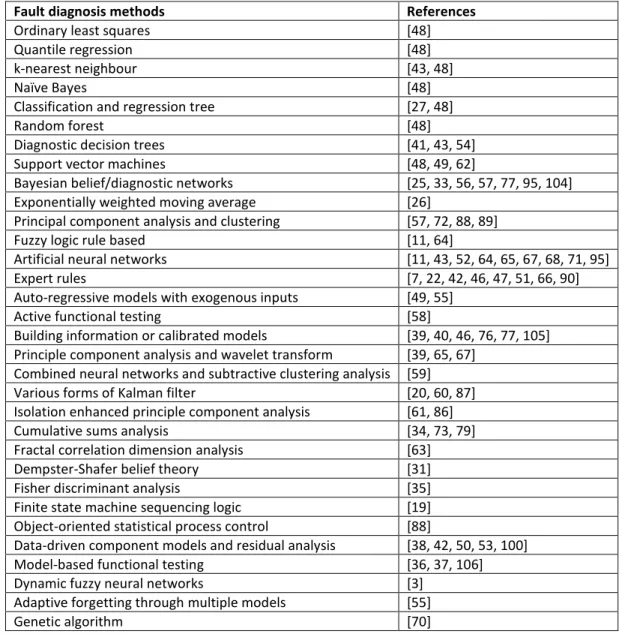
Once a fault in a system (e.g., AHU, VAV) is detected, various methods can be utilized to isolate its root-cause (e.g., broken actuator, inappropriate setpoint). The diagnosis methods reviewed in the literature are vastly fragmented. Table 3 lists 32 methods from about 80 papers. Some of the methods were

Table 2: Categorization of the faults in terms of their impact on energy use, comfort, and peak loads. The faults that affect the comfort of a more than one thermal zone are defined to have high visibility, those that affect the comfort of a single thermal zone are defined to have medium visibility, and those that do not affect comfort are

defined to have low visibility.

Fault Comfort Energy use Peak load Scale Visibility Type AHU coil valve stuck open ↓ ↑ ↑ Floor/Building High Hard AHU coil valve stuck closed ↓ ↓ ↓ Floor/Building High Hard AHU coil valve stuck partially open ↓ ↑ – Floor/Building High Hard AHU coil leaky valve – ↑ ↑ Floor/Building Low Hard AHU unstable coil valve control – – ↑ Floor/Building Low Hard AHU coil undersized coil ↓ ↓ ↓ Floor/Building High Hard

AHU coil fouling ↓ ↓ ↓ Floor/Building High Hard

AHU outdoor air intake damper stuck open – ↑ ↑ Floor/Building Low Hard AHU outdoor air intake damper stuck closed ↓ ↓ ↓ Floor/Building High Hard AHU return air damper stuck open ↓ ↓ ↓ Floor/Building High Hard AHU return air damper stuck closed – ↑ ↑ Floor/Building Low Hard AHU exhaust air damper stuck open – ↑ ↑ Floor/Building Low Hard AHU exhaust air damper stuck closed ↓ ↓ ↓ Floor/Building High Hard AHU supply air temperature bias – ↑ o ↓ ↑ o ↓ Floor/Building Low Hard AHU return air temperature bias – ↑ o ↓ ↑ o ↓ Floor/Building Low Hard AHU mixed air temperature bias – ↑ o ↓ ↑ o ↓ Floor/Building Low Hard AHU supply air pressure sensor bias ↓ o – ↓ o ↑ ↓ o ↑ Floor/Building High or Low Hard AHU other sensors (CO2, RH) ↓ o – ↓ o ↑ ↓ o ↑ Floor/Building High or Low Hard

AHU fan efficiency degradation – ↑ ↑ Floor/Building Low Hard AHU fans stuck at constant rate ↓ ↓ o ↑ ↓ o ↑ Floor/Building High or Low Hard AHU return fan complete failure – ↑ – Floor/Building Low Hard AHU supply fan complete failure ↓ ↓ ↓ Floor/Building High Hard

AHU duct fouling – ↑ ↑ Floor/Building Low Hard

AHU duct leakage – ↑ ↑ Floor/Building Low Hard

AHU fouling or broken filter – ↑ or ↓ ↑ or ↓ Floor/Building Low Hard AHU min. outdoor airflow setpoint inappropriate – or ↓ ↑ or ↓ ↑ or ↓ Floor/Building Low or High Soft AHU max. airflow setpoint inappropriate – or ↓ ↑ or ↓ ↑ or ↓ Floor/Building Low or High Soft AHU max. outdoor airflow setpoint inappropriate – ↑ ↑ Floor/Building Low Soft AHU supply air temperature setpoint too low – or ↓ ↑ or ↓ ↑ or ↓ Floor/Building Low or High Soft AHU supply air temperature setpoint too high – or ↓ ↑ or ↓ ↑ or ↓ Floor/Building Low or High Soft AHU inappropriate scheduling of fans and coils – or ↓ ↑ or ↓ ↑ or ↓ Floor/Building Low or High Soft Zone VAV reheat or heater valve stuck open ↓ ↑ ↑ Zone Medium Hard Zone VAV reheat or heater valve stuck closed ↓ ↓ ↓ Zone Medium Hard Zone VAV reheat fouled reheat coil ↓ ↓ ↓ Zone Medium Hard

Zone VAV leaky valve – ↑ ↑ Zone Low Hard

VAV damper stuck ↓ ↑ or ↓ ↑ or ↓ Zone Medium Hard VAV zone indoor temperature sensor bias ↓ ↑ or ↓ ↑ or ↓ Zone Medium Hard VAV discharge air pressure sensor bias – or ↓ ↑ or ↓ ↑ or ↓ Zone Low or Med. Hard Other sensors (CO2, RH, occupancy, photosensors) – or ↓ ↑ or ↓ ↑ or ↓ Zone Low or Med. Hard

Min. airflow setpoint inappropriate – or ↓ ↓ ↓ Zone Medium Soft Max. airflow setpoint inappropriate – or ↓ ↑ or ↓ ↑ or ↓ Zone Medium Soft Inappropriate zone temperature setpoint ↓ ↑ or ↓ ↑ or ↓ Zone Medium Soft Inappropriate temperature setback scheduling – or ↓ ↑ or ↓ ↑ or ↓ Zone Low or Med. Soft

designed to have low computational requirements to ensure that they can be deployed inside commercial building controllers (e.g., cumulative sum method [6, 79]), whereas some others were designed to be used inside building energy management systems or BAS data archivers (e.g., [99]). According to Katimapula et al. [54], developing methods that rely on existing control infrastructures, despite their computational, analytical, sensing-related limitations, is crucial for their use outside of research. Most of the fault diagnosis methods in the literature rely on pure statistical approaches such as artificial neural networks, support vector machines, principle component analysis and wavelet transform, cumulative sums analysis, auto-regressive models with exogenous inputs. Only a few studies [38, 42, 50, 53, 60, 70, 87, 100] attempted to characterize the BAS data by using the underlying physical processes through greybox modelling. Predominantly, the diagnoses of faults in the reviewed literature

Table 3: Methods used to diagnose faults in the reviewed literature. Fault diagnosis methods References

Ordinary least squares [48]

Quantile regression [48]

k-nearest neighbour [43, 48]

Naïve Bayes [48]

Classification and regression tree [27, 48]

Random forest [48]

Diagnostic decision trees [41, 43, 54] Support vector machines [48, 49, 62]

Bayesian belief/diagnostic networks [25, 33, 56, 57, 77, 95, 104] Exponentially weighted moving average [26]

Principal component analysis and clustering [57, 72, 88, 89]

Fuzzy logic rule based [11, 64]

Artificial neural networks [11, 43, 52, 64, 65, 67, 68, 71, 95] Expert rules [7, 22, 42, 46, 47, 51, 66, 90] Auto-regressive models with exogenous inputs [49, 55]

Active functional testing [58]

Building information or calibrated models [39, 40, 46, 76, 77, 105] Principle component analysis and wavelet transform [39, 65, 67]

Combined neural networks and subtractive clustering analysis [59] Various forms of Kalman filter [20, 60, 87] Isolation enhanced principle component analysis [61, 86] Cumulative sums analysis [34, 73, 79] Fractal correlation dimension analysis [63] Dempster-Shafer belief theory [31] Fisher discriminant analysis [35] Finite state machine sequencing logic [19] Object-oriented statistical process control [88]

Data-driven component models and residual analysis [38, 42, 50, 53, 100] Model-based functional testing [36, 37, 106] Dynamic fuzzy neural networks [3]

Adaptive forgetting through multiple models [55]

Genetic algorithm [70]

were undertaken via a passive approach in which control signals were not generated for commissioning pu poses. Alte ati e to a aiti g a uildi g’s atu al ope atio to p o ide ade uate i fo atio , a active (e.g., curiosity-based) commissioning approach can be adopted for hard-faults [101-103]. As such,

infrequently, AOGC routines can open/close valves and dampers automatically to inspect and to accelerate the fault diagnoses process.

Fault diagnoses method development inevitably requires a dataset to test the accuracy and appropriateness of the proposed approach. Table 4 categorizes the datasets used in the reviewed studies in three groups: (1) datasets with naturally occurring faults; (2) datasets with artificially induced faults; and (3) datasets created using a simulation tool (e.g., EnergyPlus, TRNSYS). About 70% of the reviewed papers rely on datasets with artificially induced faults (Group 2 or 3). Several studies share the same public datasets with artificially induced faults such as the ASHRAE RP 1312 [16]. The handicap of using artificially induced faults generated by using simulation tools is that errors associated with the si ulatio tools’ a ilit to i i a tual uildi g s ste s p opagate i to the datasets i a e ulous a . The limitations of the artificially-induced datasets created through field or lab experimentation are as follows:

1) Most of the common building faults are not binary (faulty and normal). For example, a valve or a damper can be stuck from 0 to 100%; a faulty coil can leak varying amounts of chilled/hot water; a d a se so ’s ias a e e s all or very large relative to its full range. The researchers inevitably make major assumptions by inducing artificial faults at some arbitrary levels during experimentation.

2) A tifi iall i du ed faults do ot p o ide a i fo atio a out a fault’s o u e e frequency. This information is important because many diagnostics approaches (e.g., Bayesian belief and decision networks) rely on a priori probability of observing a fault [25]. In addition, occurrence frequency information of faults is essential for prognostics applications [4, 5].

The shortcomings of relying on a naturally occurring dataset can be listed as follows:

1) Collecting a dataset with statistically meaningful amount of fault observations is a time-consuming process. Most of the studies that rely on naturally occurring fault datasets are small case studies with a few illustrative faults.

2) There is no guarantee that all naturally occurring faults can be captured in the dataset. As a result, it is hard to distinguish faulty operation data from normal operation data.

Table 4: Type of symptom dataset.

Symptom dataset References

Naturally occurring from field data [25, 31, 34, 37, 38, 44-46, 53, 61, 72, 77, 79, 86, 88, 89, 100, 105] Artificially induced from

experimental data

[26, 28, 30, 31, 35-39, 42, 44, 47, 49, 50, 55-57, 60, 64, 66, 67, 71, 73, 87, 104]

Artificially induced from simulation [7, 11, 19, 32, 40, 41, 43, 46, 52, 54, 57-59, 61-63, 68, 69, 87, 107]

3.

Case study

The review of the literature pointed out following research needs: (1) Fault detection has been typically relying on residual-based approaches which suffers from distinguishing random modelling errors from systemic deviation due to faults; (2) Fault isolation has been commonly relying on pure-statistical methods neglecting the potential of assimilating data within the underlying physical processes; (3) Fault diagnostics methods have been predominantly focussing on physical faults in the AHUs; and faults at the VAV thermal zones and soft faults in AHUs were addressed only in a few case studies. In this study, we put forward an inverse greybox modelling-based automated commissioning approach which attempts to address these research needs by looking at the estimated parameters of a greybox model (in lieu of residuals) to detect and diagnose operational issues and employing algorithms to train these models so that they can be used to characterize both soft and hard faults in AHUs and VAVs. Subsection 3.1 presents an overview of the building and the dataset used in this case study. Subsection 3.2 and 3.3 present the inverse modelling results for the AHU and the VAV zones, respectively. In Subsection 3.4, we discussed the weaknesses of the inverse modelling-based AOGC approach and developed future work recommendations.

3.1. Building and the dataset

The case stud is o du ted usi g a si o ths’ o th of BAS dataset archived from a large office building in Ottawa, Canada. The uildi g’s floor area is 45,123 m2. It was originally built in 1952. The HVAC equipment and control infrastructures were retrofitted at multiple stages between 2008 and 2012. The heating and cooling to the building are provided from a central heating and cooling plant serving steam and chilled water. The building has 14 AHUs that serve either VAV terminal units or perimeter induction heating units. One of the 14 AHUs was randomly selected in this case study. The selected AHU serves 32 VAV thermal zones. Of them, 13 are perimeter and 19 are core zones. Figure 1 presents the distribution of these thermal zones and the floor layout. The floor area is 816 m2– on average one zone per 25 m2. Exterior window area represents 30% of the total façade area. Sensor and actuator data from the AHU and VAVs were permanently stored in a commercial data archiver at 30 min timesteps – accessible through a Web API. Figure 2 presents sensor and actuator data types monitored in this study. The AHU does not have a heating coil. The heating is provided only to the perimeter zones through perimeter induction units. The existing control infrastructure was not upgraded – i.e., new sensors were not added or the existing ones were not calibrated for this study.

3.2.

Inverse greybox modelling of the AHU

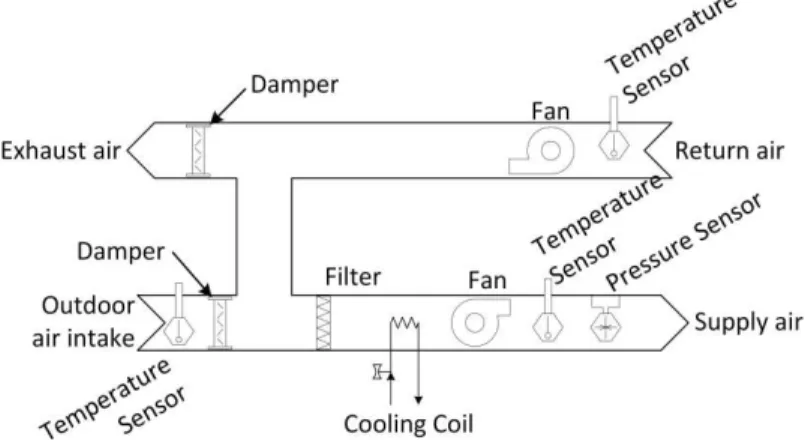
A schematic of the AHU of the case study is shown in Figure 3. As previously mentioned, it does not have a heating coil. Its primary purpose is to cool and provide outdoor air to the 32 zones. The sensors available for inverse modelling are the return, supply, and outdoor air temperatures, and the supply air pressure. The dampers and the cooling coil valve are actuated to maintain the supply air temperature setpoints – which varies between 16 and 20°C depending on the return air temperature. Supply air pressure was measured after the supply fan (variable speed) and it was always under 200 Pa. The supply fan and the cooling coil valve were scheduled to be available between 6 am and 5 pm on weekdays only.

Figure 1: The floor layout and the distribution of the thermal zones.

The objective of the inverse greybox modelling is to derive a mathematical representation of the heat-mass balance, parameters estimates of which will provide meaningful insights about the way AHU operates. In this case study, we would like our inverse model to help us understand the outdoor air fraction and the amount of sensible cooling provided by the cooling coil. A static heat-mass balance for the AHU can be formulated as follows:

(1)

where ̇ (kg/s) is the air mass flow rate, cair (J/kg-°C) is the specific heat of air, and T (°C) is the air temperature. The subscripts oa, r, and s represent outdoor air, return air, and supply air, respectively. Note that the outdoor air fraction roa equals , and thus, eqn. (1) becomes . The heat added by the fan to supply air is neglected, because the

temperature rise across a low-pressure fan ΔTfan is expected to be small relative to the precision of a typical commercial-grade temperature sensor (i.e., [108], ηfan is the fan efficiency).

Figure 3: A schematic of the AHU.

We are interested in two sets of roa values, one for scheduled operating hours (i.e., between 6 am and 5 pm on weekdays) and one for after-hours. In addition, the supply air mass flow rate is assumed proportional to the square-root of the supply air pressure ( ) (e.g., based on Bernoulli equation and assuming constant air density [108]). As described in [70], the heat input from the coil is assumed to have a power-law relationship with the cooling coil valve position (0 for closed and 100 for open). The data-driven model became as follows:

(2)

where BoptSch is a binary operating hours indicator that takes the value one between 6 am and 5 pm on weekdays and otherwise zero, and x1 to x4 are the unknown parameters of the model. The unknown





   

oa air oa r air r cc oa r air s

m c T m c T Q m m c T







_{ }

_

air air fan P T P Pa c













 

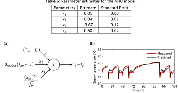
parameters of the model were solved by using the least-squares method. The model parameters were solved by partitioning the batch data for different outdoor temperature ranges: below 10°C, between 10°C and 20°C, and above 20°C. In all cases, the estimated parameters did not exhibit a noticeable variation. Table 5 lists these parameter estimates. Figure 4 illustrates this simple model and its predictive accuracy. Its predictive accuracy was tested upon a one-week worth of data retained for validation purposes (not used for model training) and found adequate (R2 0.87).

Table 5: Parameter estimates for the AHU model. Parameters Estimate Standard Error

x1 0.01 0.00

x2 0.04 0.01

x₃ -3.67 0.12

x4 0.68 0.02

(a) (b)

Figure 4: An illustration of (a) the static non-linear model for the AHU and (b) its predictive accuracy over a representative one-week period (R2 is 0.87 on the data retained for the testing purposes).

Note that the estimates for x1+x2 represent the mean outdoor air fraction during operating hours and the estimates for x1 represent the mean after-hours outdoor air fraction. During the operating hours, the outdoor air fraction roa was estimated about 5%, and during after-hours it was about 1%. Given that these values remained same for all outdoor temperature levels, it is likely that an economizer was not programmed or the outdoor air damper stuck at a nearly-closed position. Later during a site-visit, we confirmed that an economizer was not programmed (i.e., year-around minimum outdoor air supply). Figure 5 presents an example that illustrates the cooling coil valve remained open, despite the fact that

outdoor air temperature was less than the supply air temperature setpoint. The term in Figure

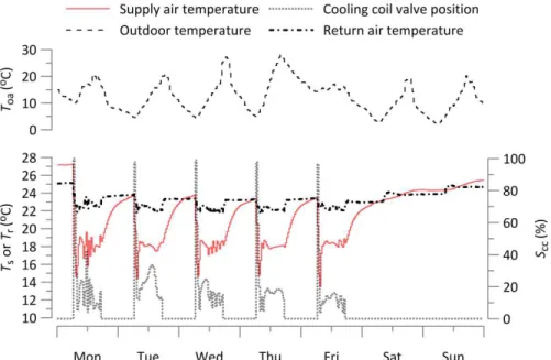
4.a with the estimated parameters x3 and x4 represents the temperature drop across the cooling coil. When the coil valve is fully open and the fan pressure is 200 Pa, the temperature drop is estimated to be 6°C. With measured maximum airflow rate of 10 m3/s (as received at each thermal zone) and assuming a constant heat capacity (1000 J/kg-°C) and density (1.2 kg/m3), the sensible cooling capacity of the coil is estimated to be 72 kW. By looking at the airflow rate and the pressure measurements, the load duration curve shown in Figure 6 was developed. The results indicate that the peak cooling loads (i.e., coil valve 100% open) occur only a small fraction of the time. Figure 5 presents an example that illustrates the stability issues in the supply air temperature control. The coil valve opens to 100% with the start of the operating schedules at 6 am, and for the rest of the day, the valve only remains at 20 to 40% position.

 

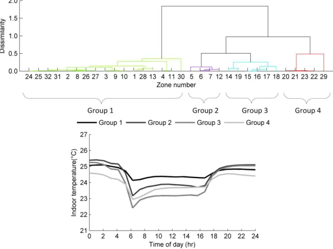
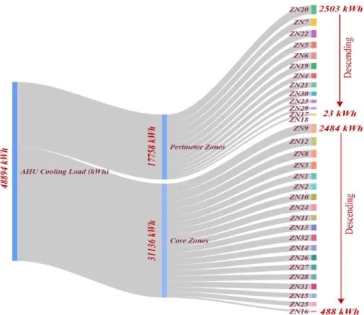
Figure 7 p ese ts a de d og a that luste s the the al zo es’ te pe atu e espo se i fou groups based on their linear correlation with each other. The mean weekday temperature results for each zone group shown in Figure 7 show the effect of the control stability issue in the AHU cooling coil valve on the thermal zones – particularly on the six zones in Group 3. Further analysis with the estimated model indicates that the peak cooling load can be reduced about 40% with a stable control loop. In addition, with the use of the estimated model, it is predicted that the presence of an economizer program can eliminate up to 25% of the cooling loads. Note that both the economizer and the cooling coil valve control loop upgrades can be undertaken at no capital cost. By knowing the airflow to each VAV zone, the breakdown of the total cooling load provided in individual zones can be estimated (see Figure 8). Simply put, the estimated AHU model acts as an approximate source of information for decision-making about immeasurable/unmeasured quantities by using the data from the existing control infrastructure – i.e., virtual metering [109]. For example, the results shown in Figure 8 (estimated by using the AHU inverse model) can help operators benchmark the cooling energy performance of thermal zones and identify the outliers (e.g., Zones 9, 20, and 18) [110].

Figure 5: An example that illustrates periods during which the outdoor temperature was lower than the supply air setpoint and the cooling coil valve was open. The example also illustrates the stability issues with the supply air

temperature control at 6 am in the morning.

Figure 7: A dendrogram clustering the measured temperature response in all 32 zones into four groups and the mean weekday temperature response for each group.

Figure 8: Distribution of the cooling energy amongst the thermal zones.

3.3.

Inverse greybox modelling of the VAV zones

Figure 9 illustrates the thermal loads affecting the perimeter and core zones of this case study. Cooling and ventilation to these zones are supplied by the AHU studied in Section 3.2. As previously mentioned, the heating is supplied through perimeter heating units. The perimeter zones gain heat through transmitted short-wave radiation from the windows, and exchange heat with outdoors due to air-infiltration and conduction through the exterior walls. In addition, an unknown amount of heat is generated due to plug-in equipment use and occupant activities. Unlike the AHU, thermal zones can have substantial thermal inertia, and thus, they need to be modelled as dynamic models. Following the inverse greybox model structure developed in [111] for perimeter spaces, a first-order dynamic model is formulated as follows:

(3)

where T (°C) is the indoor temperature, Qsol (W/m 2

) is the horizontal solar irradiance (taken from a local weather station), Bocc is a binary occupancy indicator (one on weekdays between 9 and 5 pm, otherwise zero), qvav (m

3

/s) is the VAV discharge airflow rate, Srads (zero for closed or one for open) is the state of the perimeter heater valve state, and Tcore,m (°C) is the mean temperature of the core zones. In eqn. (3), process noise (w) is a standard Wiener process and v is the measurement error. Tm (°C) is the measured indoor temperature. The x1 to x6 are the unknown parameters of the model. The unknown parameters

x1-6 and the state T are solved by using an Extended Kalman Filter. In a state-space representation, it is













          

 

,

oa sol occ s vav rads core m

m

T T T T x Q x B x T T q x S x T T x dw

customary to choose a reasonable measurement error to avoid the process model overfit the observations – i.e., to slow down the parameter learning rate in recognition of the limited power of updating parameters with a single measurement. Thus, the measurements were assumed to be corrupted by an additive Gaussian white noise (v) with standard deviation 0.1°C. This 0.1 value was selected upon conducting a sensitivity analysis between 0 and 0.5°C.

(a)

(b)

Figure 9: An illustration of the thermal loads affecting (a) perimeter and (b) core zones.

When the parameters of these perimeter zone models are estimated, the physical significance of model can be interpreted as follows: The rate of change in the indoor temperature (1) due to the heat exchange between indoors and outdoors equals , (2) due to solar gains equals , (3) due to casual gains equals , (4) due to conditioned airflow from the VAV terminal unit equals , (5) due to the heat added by the perimeter heaters equals , and (6) due to the heat exchange between the zone and the core zones equals . For core zones, the eqn. (3) is reduced to the following form:

(4)

where Tprmtr,m (°C) is the mean temperature of the perimeter zones.





















(a) (b)

Figure 10: An illustration of the dynamic model for the (a) perimeter and (b) core thermal zones.

An Extended Kalman Filter was employed recursively to update the unknown parameters. After training the model with one-month worth of data, the parameter learning process was interrupted at random instances at every week and the parameters learned up to that point were used to make three-day ahead offline predictions with the model. For example, the parameters learned until 22nd day were used to make predictions between 22nd and 25th days. The purpose of this exercise was to assess the predictive accuracy of the model and the parameter estimation approach. Figure 11 presents an example of the predictive accuracy of the models in one of the perimeter zones. For each of the 32 zones, the root-mean-squared-error (RMSE) of the model over the three-day offline prediction horizons ranged between 0.3°C to 0.7°C. This was considered acceptable.

Figure 11: Illustration of the predictive accuracy of the 1st order dynamic models trained with the Extended Kalman Filter in a representative thermal zone.

Figure 12 and Figure 13 present the estimated parameter values of the inverse greybox perimeter and core zone models, respectively. By looking at the parameter x1 (the link between indoor and outdoor temperature difference on indoor temperature), three thermal zones (20, 21, 23) appeared to be a good candidate for an envelope retrofit (e.g., sealing drafty exterior windows and doors). In two thermal zones (20, 21), by looking at the parameter x2, the solar gains appeared to play a substantial role in their temperature response. Relatively high x3 values in Zones 3, 8, 15, 20 and 22 can be interpreted as these zones are exposed to high plug-in equipment loads; whereas relatively low x3 value for Zone 26 can be interpreted as an indication of an unoccupied space. For the estimates of x4 (the link between heat added from VAV units and the indoor temperature) and x5 (the link between radiant panel state and the indoor temperature), only positive values are physically meaningful. The negative x4 value detected in Zone 23 appeared to be an indication of a faulty VAV damper or a pressure sensor. Figure 14 presents a three-day period during which the detected fault is visible. Note that the pressure sensor of the VAV unit 23 read non-zero values prior to the start of the supply fan at 6 am. With the start of the supply fan, the pressure sensor reading increased, albeit by about 30% only. On two of the three days, with the shutdown of the supply fan at 5 pm, the pressure reading fell to zero for about 30 min. Then, it

increased despite the fact that the damper position did not change and the supply fan was turned off. Later during a site visit, the problems related with this VAV unit were realized to be intermittent such that the symptoms shown in Figure 14 were visible only a fraction of the time – and as a result they were not detected by the operator. Very small x4 values shown in Zones 28, 31, and 32 appeared to be a i di atio of a VAV u it’s i a ilit to ha ge i doo te pe atu e as the damper stuck at a nearly closed position. However, we were not able to confirm these VAV issues, because the permissions of the tenants using these spaces were not granted. In a similar fashion, the negative x5 values (the link between radiant panel state and the indoor temperature) can be interpreted as an indication of a faulty perimeter heater valve. During the site visit, we were able to verify only one of the perimeter heater issues – again due to limited access to the monitored spaces.

Figure 12: Parameter estimates for the models in perimeter zones. The hatched bars (in red) represent parameters indicating a fault or an envelope issues.

Figure 13: Parameter estimates for the models in core zones. The hatched bars (in red) represent parameters indicating a fault.

Figure 14: A period during which the fault detected in VAV terminal unit 23 visible from the time-series data.

3.4. Unresolved issues

The case study is merely intended to introduce and demonstrate the capabilities of inverse greybox modelling-based AOGC approaches. Although the results were promising, because the case study was

not carried out with a comprehensive and verified fault-symptom dataset, the readers should be precautious while extrapolating the results to other use cases. We listed some of these unresolved issues as future work recommendations:

1) Table 6 lists the sub-systems in a typical VAV-AHU configuration, and it illustrates the relationships between the parameters of the inverse greybox AHU and VAV models and these subsystems. Based on these relationships, we were able to identify several issues in the AHU and VAVs; and some of them were verified during a site visit. However, comprehensive fault-symptom datasets are needed to establish cause-effect relationships between model parameters and common building faults. Even then, it is unsure whether or not the method can diagnose multiple faults affecting the model parameters simultaneously.

2) The method cannot identify issues in AHU on/off and VAV zone temperature setback schedules and zo e te pe atu e setpoi ts. These e ui e i puts f o o upa s hedules a d o upa ts’ temperature preferences. We need zone and AHU level occupancy sensing to improve scheduling decisions; and we may use thermostat keypress data as a po fo the use s’ te pe atu e preferences [20].

3) The AHU and VAV inverse models used in this case study are merely two examples. Different inverse models that can better assimilate BAS data within the physics of the heat and mass transfer problem in building components should be examined. The sensor data types needed to train these models, and the right level of model complexity should be studied. New inverse greybox models should be tailored such that their parameters become easy to communicate with domain experts.

4) While training the AHU model, as it was a static model, we employed the least-squares method to estimate the parameters. For the VAV zone models, as they were dynamic models, we employed the Extended Kalman Filter for parameter estimation. Although these decisions were based on the literature [111, 112], there are numerous alternatives such as the Unscented and Ensemble Kalman Filters and the Particle Filters [113]. We should explore to find out the parameter estimation methods best suited for inverse models used in AOGC.

5) Fault prioritization was not studied in this case study. Future work should consider how detected faults can be prioritized (e.g., in terms of their impact on comfort, energy use, peak loads, operating costs).

Table 6: Sub-systems in a typical VAV-AHU configuration, and the relationship between the inverse greybox model parameters of the AHU (Section 3.2) and the VAV zones (Section 3.3) and the performance of these sub-systems.

Systems Examples from the case study AHU Model VAV Model x1 x2 x3 x4 x1 x2 x3 x4 x5 x6

AHU coil Improper valve tuning ✓ ✓ AHU dampers Improper max. outdoor airflow rate ✓ ✓ AHU fan, filters, ductwork — ✓ ✓

AHU sensors — ✓ ✓ ✓ ✓

VAV zone perimeter heaters Valves stuck closed ✓ VAV terminal unit Faulty pressure sensor ✓ VAV zone temp. sensor — ✓ ✓ ✓ ✓ ✓ ✓

4.

Conclusions and future work

Automated on-going commissioning represents great potential to reduce operating costs, and enhance energy efficiency and comfort in buildings with connected and distributed sensor networks. In the past 20 years, a substantial research effort has been devoted into creating methodologies to diagnose operational issues from existing sensor networks. In this paper, we conducted a critical review of the literature on automated on-going commissioning approaches for air-handling units and variable air volume terminal units.

The fault detection methods have been typically built upon comparing the discrepancy between the expected and real performance of a system (i.e., residuals). The expected performance indicators are determined through expert rules or physics or data-driven models. The challenge of relying on residual-based fault detection methods is distinguishing random errors from systemic performance deviations due to faults.

The literature on fault isolation was vastly fragmented. About 80 studies reviewed in this paper employed more than 30 different fault isolation approaches. These approaches have been commonly developed as pure-statistical methods neglecting the potential of assimilating the data within the underlying physical processes.

About one-third of the reviewed studies rely on datasets generated from simulation tools such as EnergyPlus and TRNSYS to test the validity of their approaches. The handicap of using artificially induced faults using simulation tools is that errors associated ith the si ulatio tools’ a ilit to i i a tual building systems propagate into the datasets in a nebulous way. More than one-third of the reviewed studies rely on artificially-induced fault datasets through field or lab experimentation, and the rest used datasets with naturally occurring faults. For standardized testing of the on-going commissioning tools, artificially-induced fault datasets through field or lab experimentation can be favourable (e.g., ASHRAE RP 1312 datasets for AHUs). However, such datasets, particularly for VAV terminal units, are scarce in the reviewed literature.

Fault diagnostics methods in the reviewed literature have been predominantly focussing on physical faults in the AHUs; and faults at the VAV thermal zones and soft faults in AHUs were addressed only in a few case studies. Here, we argue that the faults associated with VAV thermal zones are less visible than AHU faults. This is because they tend to affect fewer occupants, and providing traditional on-going commissioning services to occupied VAV zones can be more invasive and challenging than AHUs which are typically located in mechanical rooms. In addition, considering the sheer volume of sensors and actuators in thermal zones, it is expected to be much costlier and more labour-intensive to conduct traditional going commissioning at the zone level than at the system level. Therefore, automated on-going commissioning research efforts should be directed towards diagnosing both soft and hard faults at the zone level.

In an effort to address some of the gaps identified in the literature, we put forward an inverse greybox modelling-based automated commissioning approach. This approach looks at the estimated parameters of the greybox models of an AHU and VAV thermal zones (in lieu of residuals) to detect and diagnose

both hard and soft faults. By using a dataset from an AHU and 32 VAV thermal zones in a large office building, we demonstrated the strengths and weaknesses of this approach. Several hard and soft faults were identified, and through a later site visit, the presence of some of these faults was verified. Future work recommendations were developed.

Acknowledgements

The work presented in this paper was partially supported by the Office of Energy Research and Development of Natural Resources Canada through its Program of Energy Research and Development (PERD).

References

[1] H. Sachs, S. Nadel, J. T. Amann, M. Tuazon, E. Mendelsohn, L. Rainer, G. Todesco, D. Shipley, and M. Adelaar, "Emerging energy-saving technologies and practices for the buildings sector as of 2004," American Council for an Energy-Efficicent Economy (ACEEE), Davis Energy Group, and

Marbek Resource Consultants, Washington, DC, Report, pp. 214-246, 2004.

[2] K. Roth, P. Llana, D. Westphalen, and J. Brodrick, "Automated whole building diagnostics,"

ASHRAE journal, vol. 47, p. 82, 2005.

[3] S. Katipamula and M. R. Brambley, "Wireless Condition Monitoring and Maintenance for Rooftop Packaged Heating, Ventilating and Air-Conditioning," in Proceedings, 2004 ACEEE

Summer Study on Energy Efficiency in Buildings, 2004, pp. 22-27.

[4] S. Katipamula and M. R. Brambley, "Review article: Methods for fault detection, diagnostics, and prognostics for building systems—a review, part II," HVAC&R Research, vol. 11, pp. 169-187, 2005.

[5] S. Katipamula and M. R. Brambley, "Review article: methods for fault detection, diagnostics, and prognostics for building systems—a review, Part I," HVAC&R Research, vol. 11, pp. 3-25, 2005. [6] J. M. Lucas, "Cumulative sum (CUSUM) control schemes," Communications in Statistics-Theory

and Methods, vol. 14, pp. 2689-2704, 1985.

[7] J. Schein, S. T. Bushby, N. S. Castro, and J. M. House, "A rule-based fault detection method for air handling units," Energy and Buildings, vol. 38, pp. 1485-1492, 2006.

[8] NRCan, "Energy use data handbook 1990 to 2010," Natural Resources Canada2013. [9] DOE, "Buildings energy data book," United States Department of Energy2011.

[10] P. F. Hutchins, "Automated Ongoing Commissioning via Building Control Systems," Energy

Engineering, vol. 113, pp. 11-20, 2016/01/01 2016.

[11] W. H. Allen, A. Rubaai, and R. Chawla, "Fuzzy Neural Network-Based Health Monitoring for HVAC System Variable-Air-Volume Unit," IEEE Transactions on Industry Applications, vol. 52, pp. 2513-2524, 2016.

[12] A. 25, "Building Optimization and Fault Diagnosis Source Book," International Energy Agency Energy in Buildings and Communities Program Annex 251996.

[13] A. 34, "Technical Synthesis Report: Computer Aided Evaluation of HVAC System Performance," International Energy Agency Energy in Buildings and Communities Program Annex 342006. [14] A. 40, "Commissioning Tools for Improved Energy Performance," International Energy Agency

Energy in Buildings and Communities Program Annex 402004.

[15] W. Anis, T. Brennan, G. Nelson, C. Olson, and D. Bohac, "ASHRAE 1478 RP: Measuring Air-Tightness of Mid-and High-Rise Non-Residential Buildings," ASHRAE Transactions, vol. 119, 2013. [16] J. Wen and S. Li, "ASHRAE RP-1312 -- TOOLS FOR EVALUATING FAULT DETECTION AND

[17] CABA, "CABA Intelligent Buildings and Big Data," Continental Automated Buildings Association2016.

[18] CanmetEnergy, "Experts research forum on intelligent buildings: final report," Natural Resources Canada, Montreal2015.

[19] J. E. Seem and J. M. House, "INTEGRATED CONTROL AND FAULT DETECTION OF AIR-HANDLING UNITS," IFAC Proceedings Volumes, vol. 39, pp. 19-24, 2006/01/01 2006.

[20] H. B. Gunay, "Improving energy efficiency in office buildings through adaptive control of the indoor climate," PhD, Civil Engineering, Carleton University, Ottawa, 2016.

[21] M. R. Brambley, N. Fernandez, W. Wang, K. A. Cort, H. Cho, H. Ngo, and J. Goddard, "FINAL PROJECT REPORT SELF-CORRECTING CONTROLS FOR VAV SYSTEM FAULTS," 2011.

[22] M. Brambley, N. Bauman, S. Katipamula, and R. G. Pratt, "Enhancing building operations through automated diagnostics: Field test results," 2003.

[23] P. Zhao, T. Peffer, R. Narayanamurthy, G. Fierro, P. Raftery, S. Kaam, and J. Kim, "Getting into the zone: how the internet of things can improve energy efficiency and demand response in a commercial building," ed, 2016.

[24] R. Attar, E. Hailemariam, S. Breslav, A. Khan, and G. Kurtenbach, "Sensor-enabled Cubicles for Occupant-centric Capture of Building Performance Data," ASHRAE Transactions, vol. 117, 2011. [25] D. Dey and B. Dong, "A probabilistic approach to diagnose faults of air handling units in

buildings," Energy and Buildings, vol. 130, pp. 177-187, 2016.

[26] H. Wang and Y. Chen, "A robust fault detection and diagnosis strategy for multiple faults of VAV air handling units," Energy and Buildings, vol. 127, pp. 442-451, 2016.

[27] R. Yan, Z. Ma, Y. Zhao, and G. Kokogiannakis, "A decision tree based data-driven diagnostic strategy for air handling units," Energy and Buildings, vol. 133, pp. 37-45, 2016.

[28] T. Mulumba, A. Afshari, K. Yan, W. Shen, and L. K. Norford, "Robust model-based fault diagnosis for air handling units," Energy and Buildings, vol. 86, pp. 698-707, 2015.

[29] Y. Yu, D. Woradechjumroen, and D. Yu, "A review of fault detection and diagnosis methodologies on air-handling units," Energy and Buildings, vol. 82, pp. 550-562, 2014.

[30] H. Wang, Y. Chen, C. W. H. Chan, J. Qin, and J. Wang, "Online model-based fault detection and diagnosis strategy for VAV air handling units," Energy and Buildings, vol. 55, pp. 252-263, 2012. [31] S. R. West, Y. Guo, X. R. Wang, and J. Wall, "Automated fault detection and diagnosis of HVAC

subsystems using statistical machine learning," in 12th International Conference of the

International Building Performance Simulation Association, 2011.

[32] S. H. Lee and F. W. H. Yik, "A study on the energy penalty of various air-side system faults in buildings," Energy and Buildings, vol. 42, pp. 2-10, 2010.

[33] M. Najafi, "Modeling and Measurement Constraints in Fault Diagnostics for HVAC Systems," ed, 2010.

[34] J. T oja o á, J. Vass, K. Ma ek, J. Rojiček, a d P. Stluka, "Fault Diag osis of Ai Handling Units,"

IFAC Proceedings Volumes, vol. 42, pp. 366-371, 2009/01/01 2009.

[35] Z. Du and X. Jin, "Multiple faults diagnosis for sensors in air handling unit using Fisher discriminant analysis," Energy Conversion and Management, vol. 49, pp. 3654-3665, 2008. [36] P. Xu, P. Haves, and M. Kim, "Model-based automated functional testing -- Methodology and

application to air-handling units," presented at the ASHRAE Winter Conference, Florida, 2005. [37] L. Luskay, M. Brambley, and S. Katipamula, "Methods for Automated and Continuous

Commissioning of Building Systems," Air-Conditioning and Refrigeration Technology Institute (US)2003.

[38] J. E. Pakanen and T. Sundquist, "Automation-assisted fault detection of an air-handling unit; implementing the method in a real building," Energy and Buildings, vol. 35, pp. 193-202, 2003.

[39] S. Li and J. Wen, "A model-based fault detection and diagnostic methodology based on PCA method and wavelet transform," Energy and Buildings, vol. 68, Part A, pp. 63-71, 2014.

[40] M. Basarkar, "MODELING AND SIMULATION OF HVAC FAULTS IN ENERGYPLUS," ed, 2013. [41] D. Holcomb, W. Li, and S. A. Seshia, "Algorithms for green buildings: Learning-based techniques

for energy prediction and fault diagnosis," Google Scholar, UCB/EECS-2009-138, 2009.

[42] P. Carling, "Comparison of three fault detection methods based on field data of an air-handling unit/Discussion," ASHRAE Transactions, vol. 108, p. 904, 2002.

[43] J. M. House, W. Y. Lee, and D. R. Shin, "Classification techniques for fault detection and diagnosis of an air-handling unit," ASHRAE Transactions, vol. 105, p. 1087, 1999.

[44] J. E. Seem, J. M. House, and R. H. Monroe, "On-line monitoring and fault detection," ASHRAE

journal, vol. 41, p. 21, 1999.

[45] D. Choinière, "Four Years of On-Going Commissioning in CTEC-Varennes Building with a BEMS Assisted CX Tool," 2004.

[46] J. M. House, H. Vaezi-Nejad, and J. M. Whitcomb, "An expert rule set for fault detection in air-handling units," Transactions-American Society Of Heating Refrigerating And Air Conditioning

Engineers, vol. 107, pp. 858-874, 2001.

[47] J. Schein, Results from field testing of embedded air handling unit and variable air volume box

fault detection tools: US Department of Commerce, Technology Administration, National

Institute of Standards and Technology, 2006.

[48] S. Frank, M. Heaney, X. Jin, J. Robertson, H. Cheung, R. Elmore, and G. Henze, "Hybrid Model-Based and Data-Driven Fault Detection and Diagnostics for Commercial Buildings," NREL (National Renewable Energy Laboratory (NREL), Golden, CO (United States))2016.

[49] Y. Zhao, J. Wen, F. Xiao, X. Yang, and S. Wang, "Diagnostic Bayesian networks for diagnosing air handling units faults – part I: Faults in dampers, fans, filters and sensors," Applied Thermal

Engineering.

[50] S.-H. Cho, H.-C. Yang, M. Zaheer-uddin, and B.-C. Ahn, "Transient pattern analysis for fault detection and diagnosis of HVAC systems," Energy Conversion and Management, vol. 46, pp. 3103-3116, 2005.

[51] S. Katipamula, M. R. Brambley, and L. Luskay, "Automated Proactive Techniques for Commissioning Air-Handling Units," Journal of Solar Energy Engineering, vol. 125, pp. 282-291, 2003.

[52] S. Wang and Y. Chen, "Fault-tolerant control for outdoor ventilation air flow rate in buildings based on neural network," Building and Environment, vol. 37, pp. 691-704, 2002.

[53] P. Xu and P. Haves, "Field testing of component-level model-based fault detection methods for mixing boxes and VAV fan systems," ed, 2002.

[54] S. Katipamula, R. G. Pratt, D. P. Chassin, and Z. T. Taylor, "Automated fault detection and diagnostics for outdoor-air ventilation systems and economizers: Methodology and results from field testing," ASHRAE Transactions, vol. 105, p. 555, 1999.

[55] H. Yoshida and S. Kumar, "ARX and AFMM model-based on-line real-time data base diagnosis of sudden fault in AHU of VAV system," Energy Conversion and Management, vol. 40, pp. 1191-1206, 1999.

[56] M. Najafi, D. M. Auslander, P. L. Bartlett, P. Haves, and M. D. Sohn, "Application of machine learning in the fault diagnostics of air handling units," Applied Energy, vol. 96, pp. 347-358, 2012. [57] R. Yan, Z. Ma, G. Kokogiannakis, and Y. Zhao, "A sensor fault detection strategy for air handling

units using cluster analysis," Automation in construction, vol. 70, pp. 77-88, 2016.

[58] M. Padilla and D. Choinière, "A combined passive-active sensor fault detection and isolation approach for air handling units," Energy and Buildings, vol. 99, pp. 214-219, 2015.

[59] Z. Du, B. Fan, X. Jin, and J. Chi, "Fault detection and diagnosis for buildings and HVAC systems using combined neural networks and subtractive clustering analysis," Building and Environment, vol. 73, pp. 1-11, 2014.

[60] W.-Y. Lee, C. Park, and G. E. Kelly, "Fault detection in an air-handling unit using residual and recursive parameter identification methods," Transactions-American Society Of Heating

Refrigerating And Air Conditioning Engineers, vol. 102, pp. 528-539, 1996.

[61] S. Wang and F. Xiao, "Sensor Fault Detection and Diagnosis of Air-Handling Units Using a Condition-Based Adaptive Statistical Method," HVAC&R Research, vol. 12, pp. 127-150, 2006/01/01 2006.

[62] X.-B. Yang, X.-Q. Jin, Z.-M. Du, Y.-H. Zhu, and Y.-B. Guo, "A hybrid model-based fault detection strategy for air handling unit sensors," Energy and Buildings, vol. 57, pp. 132-143, 2013.

[63] X.-B. Yang, X.-Q. Jin, Z.-M. Du, and Y.-H. Zhu, "A novel model-based fault detection method for temperature sensor using fractal correlation dimension," Building and Environment, vol. 46, pp. 970-979, 2011.

[64] J. Du, M. J. Er, and L. Rutkowski, "Fault Diagnosis of an Air-Handling Unit System Using a Dynamic Fuzzy-Neural Approach," in Artificial Intelligence and Soft Computing: 10th

International Conference, ICAISC 2010, Zakopane, Poland, June 13-17, 2010, Part I, L. Rutkowski,

R. Scherer, R. Tadeusiewicz, L. A. Zadeh, and J. M. Zurada, Eds., ed Berlin, Heidelberg: Springer Berlin Heidelberg, 2010, pp. 58-65.

[65] Z. Du, X. Jin, and Y. Yang, "Fault diagnosis for temperature, flow rate and pressure sensors in VAV systems using wavelet neural network," Applied Energy, vol. 86, pp. 1624-1631, 2009. [66] H. Yang, S. Cho, C.-S. Tae, and M. Zaheeruddin, "Sequential rule based algorithms for

temperature sensor fault detection in air handling units," Energy Conversion and Management, vol. 49, pp. 2291-2306, 2008.

[67] Z. Du, X. Jin, and Y. Yang, "Wavelet Neural Network-Based Fault Diagnosis in Air-Handling Units,"

HVAC&R Research, vol. 14, pp. 959-973, 2008/11/01 2008.

[68] W.-Y. Lee, J. M. House, and N.-H. Kyong, "Subsystem level fault diagnosis of a building's air-handling unit using general regression neural networks," Applied Energy, vol. 77, pp. 153-170, 2004.

[69] J. Du and E. Meng Joo, "An artificial intelligence approach towards fault diagnosis of an air-handling unit," in 2004 5th Asian Control Conference (IEEE Cat. No.04EX904), 2004, pp. 1594-1601 Vol.3.

[70] M. Padilla, D. Choinière, and J. A. Candanedo, "A model-based strategy for self-correction of sensor faults in variable air volume air handling units," Science and Technology for the Built

Environment, vol. 21, pp. 1018-1032, 2015/10/03 2015.

[71] W.-Y. Lee, J. M. House, C. Park, and G. E. Kelly, "Fault diagnosis of an air-handling unit using artificial neural networks," Transactions-American Society Of Heating Refrigerating And Air

Conditioning Engineers, vol. 102, pp. 540-549, 1996.

[72] Z. Du, X. Jin, and X. Yang, "A robot fault diagnostic tool for flow rate sensors in air dampers and VAV terminals," Energy and Buildings, vol. 41, pp. 279-286, 2009.

[73] J. Schein and J. M. House, "Application of control charts for detecting faults in variable-air-volume boxes," Transactions-American Society Of Heating Refrigerating And Air Conditioning

Engineers, vol. 109, pp. 671-682, 2003.

[74] D. Westphalen, K. Roth, and J. Brodrick, "Duct leakage fault detection," ASHRAE journal, vol. 47, p. 56, 2005.

[75] N. Djuric and V. Novakovic, "Review of possibilities and necessities for building lifetime commissioning," Renewable and Sustainable Energy Reviews, vol. 13, pp. 486-492, 2009.