Emerging cell array based on reaction-diffusion

ORIGINAL ARTICLE DOI 10.1007/s10015-006-0394-8

Shuhei Miyashita · Satoshi Murata

Emerging cell array based on reaction–diffusion

Received and accepted: July 4, 2006

Abstract This article demonstrates the self-replication and

self-organization phenomena based on a reaction–diffusion mechanism by computer simulation. The simulation model consists of a one-dimensional cell array. Each cell contains two kinds of chemical substances, activator u and inhibitor v, that can generate a reaction–diffusion wave, which is a spatial concentration pattern. The cells are supposed to be divided or deleted depending on the concentrations of chemical substances. We tried several kinds of diffusion coefficient in the model, and in some simulations, a self-replication process and a generating cell array with a meta-bolic process were observed. By applying the division rule and the apoptosis rule, cell arrays duplicate in two oscillat-ing states, i.e., self-replication processes were observed. By applying a division rule and an annihilation rule, a cell array that has a stable length is generated by changing the cell components, i.e., generating a cell array by a metabolic process was observed. Surprisingly, these two phenomena are realized independently of the initial number of cells.

Key words Reaction · Diffusion · Morphogenesis

Introduction

The self-replication and self-organization abilities of multi-cellular organisms are among the most fundamental charac-teristics that discriminate creatures from non-creatures. As each cell contains the same genome, this feat is realized in a distributed and autonomous way in the absence of

central-ized control. However, in spite of the great progress that has been made in molecular biology over the past few decades, the overall picture of the principles behind the spatiotempo-ral dynamics of these processes is still lacking. In 1952, A.M. Turing advocated a reaction–diffusion mechanism, and sug-gested that this mechanism, which is a kind of spatial con-centration pattern, plays a key role in forming a periodic shape in a small creature called a hydra.1

L. Wolpert2 sug-gested a concept of positional information because he thought that cells need to recognize themselves by their position because they all have identical genes. C.G. Langton built a cellular automata model of self-replication (SRloops) on a two-dimensional cell array. As the model consists of discrete internal states with finite state automata, it is not easy to relate this model to the biological cell. K. Tomita et al.4

created graph automata, which gave a description of the dynamic topological change in a cell net-work. They extended the concept of cellular automata to certain graphs of cells. This model is able to describe mor-phological changes such as cell division or cell death, but little attention has been given to a relation between mor-phogenetic processes and a reaction–diffusion mechanism.

Model

Reaction–diffusion

In this research, a one-dimensional cell array model was chosen for simplicity. Figure 1 shows a schema of the model. These nodes represent cells containing two kinds of chemi-cal substance, activator u and inhibitor v, that can generate a reaction–diffusion wave. These two chemicals react with each other and diffuse into neighboring cells according to the concentration gradient.

dur dt= +5u tr

( )

−6v tr

( )

+ +1 D uu

{

r−1

( )

t +ur+1

( )

t −2u tr

( )

}

(1)

dvr dt= +6u tr

( )

−7vr+ +1 D vv

{

r−1

( )

t +vr+1

( )

t −2v tr

( )

}

(2) The reaction–diffusion model that we use is the same as Turing’s, which is expressed as partial differential Eqs. 1

S. Miyashita (*)

Department of Informatics, University of Zurich, Andreasstrasse 15, CH8050 Zurich, Switzerland

Tel. +41-44-635-4589; Fax +41-44-635-45-07 e-mail: miya@ifi.unizh.ch

S. Murata

Tokyo Institute of Technology, Yokohama, Japan

This work was presented in part at the 11th International Symposium on Artificial Life and Robotics, Oita, Japan, January 23–25, 2006

and 2, where ur and vr represents the concentration of activator and inhibitor, respectively, with subscript r as an identification number. Du and Dv represent the diffusion

constants of the activator and inhibitor, respectively (Du=

0.7, Dv= 1.2). Dirichlet boundary conditions were applied to

the system, which set the chemical concentration at the boundary to zero. The initial concentrations were set as the equilibrium point (u, v) = (1.0, 1.0).

Cell cycle and cell differentiation

Since the cell cycle is determined by various factors, in this article the cell cycle is supposed to be generated synchro-nously. Figure 2 represents the cell cycle in the model. Every cell has an interphase and a mitotic phase in the cycle. In the mitotic phase, reaction and diffusion of the chemical substances take place. In the interphase, cells are differentiated depending on the chemical concentrations (see below).

Figure 3 shows the cell differentiation rules. Cell division (top) takes place when the concentration of the activator becomes greater than a specific threshold (the division threshold, set as 1.5) in the mitotic phase. The cell divides into two cells, and the concentration of each chemical sub-stance immediately before division is their concentration in each divided cell.

Conversely, the annihilation rule (middle) is activated when the concentration of the activator becomes lower than another specific threshold (the annihilation threshold, set as 1.0) in the mitotic phase. In this rule, one cell is deleted, but the connection of the other two cells remains. The apoptosis rule (bottom) is similar to the annihilation rule, and is

acti-vated when the concentration of the activator becomes smaller than that of the inhibitor in the same phase. The system is then divided into two separate groups by cell deletion. Every differential equation is integrated by the Runge–Kutta method (∆ t = 0.01, 1 step = 100 ∆ t, 1 inter-phase corresponds to 150 steps).

Simulations and results

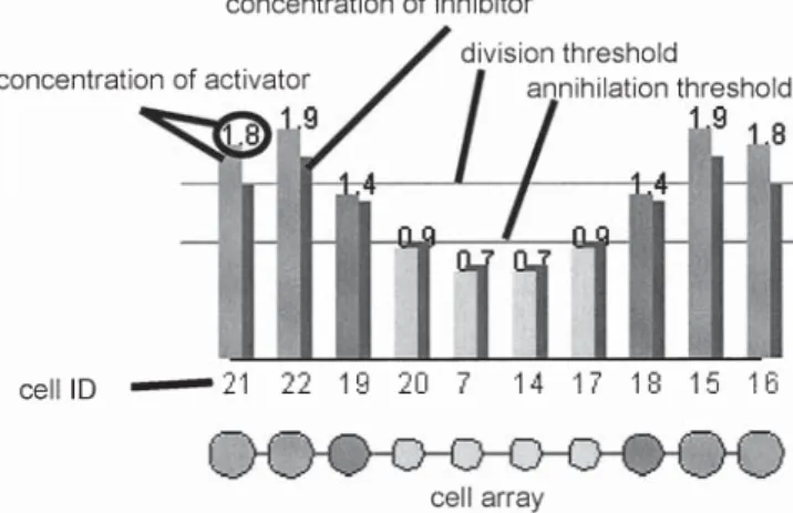
In the computer simulations, eqs. 1 and 2 and the cell differ-entiation rules are simulated synchronously according to the cell cycle. Figure 4 shows the simulation model. The bars above each cell represent the concentrations of activa-tor and inhibiactiva-tor. The concentrations of the activaactiva-tor are displayed in front, and those of the inhibitor are displayed behind. The values of the concentrations of the activator are

Fig. 1. One-dimensional cell array

Fig. 2. Cell cycle

Fig. 3. Cell differentiation

presented on each shoulder of the bar. The division thresh-old, annihilation threshthresh-old, and identification numbers of the cells are also listed.

Self-replication process

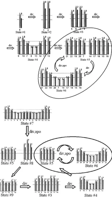
In this model, the division rule and the apoptosis rule are applied in the mitotic phase. Figure 5 shows the self-replication process when we settled on one cell as the initial condition. In the first stage, cell divisions are repeated twice

in the mitotic phase, and the initial cell grows into 8 cells (state 1 to state 4). Then the apoptosis rule is activated, four cells positioned at the center (cells 8 and 13 in state 4) are deleted, and four cells at the side (cells 9–12 in state 4) are divided. Consequently, the system duplicates itself by oscil-lating between state 5 and state 6.

Figure 6 shows the case where the initial number of cells is larger than the oscillating number 10 (state 7). The phe-nomenon that the final state converges to states 5 and 6 is observed.

Fig. 5. A self-replication process in one cell

Fig. 6. A self-replication process from 15 cells

Fig. 7. A cell array generating by a metabolic process from one cell

Generating a cell array with a metabolic process

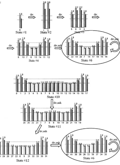
The division rule and the annihilation rule are applied in the mitotic phase. Figure 7 shows that the number of cells increases to 10 according to the cell division rule. In the mitotic phase at state 6, four cells positioned at the center (cells 20,7,14 and 17 in state 6) are annihilated, and another four cells (cells 21,22,15, and 16) at the sides are divided. Finally, the number of cells remains stable at 10. The system perpetually produces new cells and replaces some old cells.

In order to investigate the stability of the process, 18 cells are set in the initial state. Figure 8 shows that the number of cells finally converges to the same pattern (state 6).

Discussion

In addition to the simulation described above, we chose different numbers of cells as the initial condition, and the results are shown in Fig. 9. The X-axis represents the num-ber of mitotic phases passed and the Y-axis represents the number of cells. This figure shows that the length of all cell arrays which start from between 1 cell and 30 cells finally converge to 10. This suggests not only that we can choose variable numbers of cells for an initial condition (at least from 1 to 30), but also that we can cut any cell connections, but we will still generate two cell arrays of size 10.

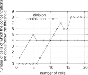
Since the patterns of reaction–diffusion waves seem to be unique to the length of the cell arrays, especially when the length is short, we counted the number of cells which exceeded the division threshold but which were below the

Fig. 8. Generating a cell array from 18 cells

Fig. 9. Transition graph of the number of cells

Fig. 10. Graph when the threshold is exceeded

Fig. 11. The number of cells in each parameter set

annihilation threshold in the first mitotic phase. The X-axis in Fig. 10 represents the number of cells, and the Y-axis represents the number of cells in which the concentrations are above (or below) the threshold. As the figure shows, when the number of cells is less than 9, the number of cells that exceed the division threshold is larger than the num-bers which are below the annihilation threshold. That is, the length becomes short in the next mitotic phase, and when the number of cells we choose is more than 11, the result is the other way round. This figure clearly shows that the system converges to 10.

Figure 11 represents the number of cells when the mi-totic phase has passed ten times with different diffusion coefficients. The initial number of cells was between 1 and 30 for each parameter set. The X and Y axes represent the diffusion coefficients Du and Dv, respectively, and the Z axis

represents the number of cells. As can be seen, the system does not always converge to one state, and although the

system shows its robustness in the event of external distur-bances by its adequate diffusion coefficients, the ranges of these parameters are narrow.

Conclusion

In conclusion, two fundamental organic behaviors, i.e., the self-replication process and generating a cell array by a metabolic process, were observed by applying a reaction– diffusion mechanism on distributed space. In the self-replication process, the phenomenon that cell arrays duplicate themselves by oscillating between two states was observed. In generating a cell array by a metabolic process, the phenomenon that a cell array which has a stable length is generated by changing its cell components was observed. This research shows the possibility that a reaction–diffusion system plays some role in controlling these vital activities of living things.

Acknowledgments We thank Peter Eggenberger Hotz for many help-ful suggestions. This research was supported by the Swiss National Science Foundation, project #200021-105634/1.

References

1. Turing AM (1952) A reaction–diffusion model for development. The chemical basis of morphogenesis. Phil Trans R Soc London, Ser B, Biol Sci 237(5):37–72

2. Wolpert L (1969) Positional information and the spatial pattern of cellular differentiation. J Theor Biol 25:1–47

3. Langton CG (1984) Self-reproduction in cellular automata. Phys D, Nonlinear Phenomena 10(1–2):135–144

4. Tomita K, Kurokawa H, Murata S (2002) Graph automata: natural expression of self-reproduction. Phys D, Nonlinear Phenomena 171(4):197–210