HAL Id: inserm-00484302
https://www.hal.inserm.fr/inserm-00484302
Submitted on 18 May 2010
HAL is a multi-disciplinary open access archive for the deposit and dissemination of sci-entific research documents, whether they are pub-lished or not. The documents may come from teaching and research institutions in France or abroad, or from public or private research centers.
L’archive ouverte pluridisciplinaire HAL, est destinée au dépôt et à la diffusion de documents scientifiques de niveau recherche, publiés ou non, émanant des établissements d’enseignement et de recherche français ou étrangers, des laboratoires publics ou privés.
models.
Johanna Lepeule, Fabrice Caïni, Sébastien Bottagisi, Julien Galineau, Agnès
Hulin, Nathalie Marquis, Aline Bohet, Valérie Siroux, Monique Kaminski,
Marie-Aline Charles, et al.
To cite this version:
Johanna Lepeule, Fabrice Caïni, Sébastien Bottagisi, Julien Galineau, Agnès Hulin, et al.. Ma-ternal exposure to nitrogen dioxide during pregnancy and offspring birth weight: comparison of two exposure models.: Comparison of Two Exposure Models to Air Pollutants. Environmental Health Perspectives, National Institute of Environmental Health Sciences, 2010, 118 (10), pp.1483-9. �10.1289/ehp.0901509�. �inserm-00484302�
HEALTH
PERSPECTIVES
HEALTH
PERSPECTIVES
National Institutes of Health
U.S. Department of Health and Human Services
Maternal Exposure to Nitrogen Dioxide during
Pregnancy and Offspring Birthweight:
Comparison of Two Exposure Models
Johanna Lepeule, Fabrice Caïni, Sébastien Bottagisi,
Julien Galineau, Agnès Hulin, Nathalie Marquis,
Aline Bohet, Valérie Siroux,
Monique Kaminski, Marie-Aline Charles, Rémy Slama,
and the Eden mother-child cohort study group
doi: 10.1289/ehp.0901509 (available at http://dx.doi.org/)
Online 14 May 2010
ehponline.org
1
Maternal Exposure to Nitrogen Dioxide during Pregnancy and
Offspring Birthweight: Comparison of Two Exposure Models
Johanna Lepeule1,2, Fabrice Caïni3, Sébastien Bottagisi1,2, Julien Galineau4, Agnès
Hulin3, Nathalie Marquis4, Aline Bohet5,6, Valérie Siroux2,7, Monique Kaminski8,9,
Marie-Aline Charles 10,11, Rémy Slama1,2 and the Eden mother-child cohort study group
1: Inserm, Avenir Team “Environmental Epidemiology Applied to Fecundity and
Reproduction”, Institut Albert Bonniot, U823, Grenoble, France
2: University J. Fourier Grenoble, Grenoble, France.
3: ATMO Poitou-Charentes, Perigny, France.
4: AIRLOR, Vandoeuvre les Nancy, France.
5: Inserm, U1018, CESP Centre de Recherche en Epidémiologie et Santé des populations,
Team Epidemiology of reproduction and child development, Le Kremlin-Bicêtre, France.
6: Univ Paris-Sud 11, UMRS 1018, Le Kremlin Bicêtre, France
7: Inserm, Team « Epidemiology of Cancer and Severe Diseases », Institut Albert Bonniot,
U823, Grenoble, France
8: UMR S953, IFR 69, Epidemiological Research Unit on Perinatal and Women's and
Children’s Health, Villejuif, France.
9: UPMC, Paris, France.
10: Inserm, U1018, CESP Centre de Recherche en Epidemiologie et Santé des Populations,
Team Epidemiology of obesity, diabetes and renal disease over the life course, Villejuif,
France.
11: University Paris-Sud 11, UMRS 1018, Le Kremlin Bicêtre, France
Corresponding author: Johanna Lepeule, johanna.lepeule@ujf-grenoble.fr, Phone: +33 476
2 Inserm, Team “Environmental Epidemiology applied to Fertility and Human Reproduction”,
U823, Institut Albert Bonniot, BP 170, La Tronche, F-38042 Grenoble CEDEX 9, France.
Running title: Comparison of Two Exposure Models to Air Pollutants
Key-words: atmospheric pollution, birthweight, cohort, exposure modeling, geostatistical,
measurement error, monitoring station, nitrogen dioxide, spatial variation, temporal variation
Abbreviations:
AQMS : Air Quality Monitoring Station
CI : Confidence Interval
LUR : Land Use Regression
NO2 : Nitrogen dioxide
TAG model : Temporally Adjusted Geostatistical model
Acknowledgements:
We thank José Labarere (CHU Grenoble) and Jean Maccario (University of Paris Descartes)
for useful discussions. We are indebted to the midwife research assistants (L. Douhaud, S.
Bedel, B. Lortholary, S. Gabriel, M. Rogeon, and M. Malinbaum) for data collection and to P.
Lavoine for checking, coding, and data entry.This project has been funded by grants from the
French agency for environmental and occupational health safety (AFSSET, call
“Environnement-Santé-Travail”) and from ADEME. The Eden cohort is funded by the
Foundation for medical research (FRM), Inserm, IReSP, Nestlé, French Ministry of health,
National Research Agency (ANR), Univ. Paris-Sud, Institute of health monitoring (InVS),
3 of Environmental Epidemiology (Inserm U823) is supported by an AVENIR grant from
Inserm.
All authors declare that they have nothing to disclose, financially or otherwise. There is no
4
Outline of manuscript -section headers
Abstract
Introduction
Materials and Methods
Study population and data collection
Exposure to NO2
Nearest air quality monitoring station model (model 1)
Temporally adjusted geostatistical model (model 2)
Statistical analyses
Spatial and temporal variations in exposure
Comparison of the exposure estimates generated by each model
Exposure-response relationship
Results
Population
Exposure to air pollutants
Associations between air pollutants and fetal growth
Discussion Conclusion References Tables Figure legends Figures
5
Abstract
Background: Studies of the effects of air pollutants on birthweight often assess exposure
with permanent air quality monitoring stations (AQMS) networks; these have a poor spatial
resolution.
Objective: We aimed to compare the exposure model based on the nearest AQMS and a
temporally adjusted geostatistical (TAG) model with a finer spatial resolution, for use in
pregnancy studies.
Methods: The AQMS and TAG exposure models were implemented in two areas surrounding
medium-sized cities in which 776 pregnant women were followed as part of the EDEN
mother-child cohort. The exposure models were compared in terms of estimated nitrogen
dioxide (NO2) levels and of their association with birthweight.
Results: The correlation between the two estimates of exposure during the first trimester of
pregnancy was r=0.67, 0.70, and 0.83 for women living within 5, 2 or 1 km of an AQMS,
respectively. Exposure patterns displayed greater spatial than temporal variations. Exposure
during the first trimester of pregnancy was most strongly associated with birthweight for
women living less than 2 km away from an AQMS: a 10 µg/m3 increase in NO2 exposure was
associated with an adjusted difference in birthweight of 37g (95% confidence interval (CI),
-75; 1g) for the nearest AQMS model and of -51g (95% CI, -128; 26g) for the TAG model.
The association was less strong (higher p-value) for women living within 5 or 1 km of an
AQMS.
Conclusions: The two exposure models tended to give consistent in terms of association with
6
Introduction
Several epidemiological studies have reported associations between maternal exposure to
nitrogen dioxide (NO2) during pregnancy and fetal growth assessed by birthweight, taking
into account gestational duration (e.g., Bell et al. 2007; Liu et al. 2007; Ritz and Wilhelm
2008; Slama et al. 2008; Wilhelm and Ritz 2003). Various approaches may be used to
estimate exposure, from the use of biomarkers of exposure to personal dosimeters and
environmental models. Most previous studies have been based on measurements from
permanent air quality monitoring stations (AQMS), using data from the AQMS closest to the
subject’s home address, or interpolating data for neighboring monitors, for which
measurements are averaged over the entire pregnancy or over each trimester of pregnancy.
This approach has the advantage of making use of readily available exposure data, being
simple to implement and, because pollutants are assessed on an hourly or at least weekly
basis, being highly flexible in terms of the temporal exposure window considered. However,
the spatial density of AQMS networks is generally low, and studies have shown that the data
provided by permanent AQMS are representative only of air pollution levels in the close
vicinity of the station (Lebret et al. 2000). Studies based on AQMS measurements assume that
air pollution levels are homogeneous within a buffer of several kilometers around each
monitor, or, at least, that exposure misclassification introduces no major bias into the
estimated exposure-response relationship. However, studies based on the simultaneous use of
several exposure models have demonstrated that the amplitude of the measurement error may
be large (Nerriere et al. 2005; Nethery et al. 2008; Sarnat et al. 2005). Moreover, at least for
respiratory or cardiovascular outcomes, measurement error may have a large impact on the
exposure-response relationship (Miller et al. 2007; Van Roosbroeck et al. 2008). This issue
7 We aimed to compare the exposure model based on the nearest AQMS and a temporally
adjusted geostatistical (TAG) model based on measurement campaigns with a fine spatial
resolution and also focusing on background pollution, in the context of a mother-child cohort.
These models were compared in terms of estimated NO2 levels and the estimated association
8
Materials and Methods
Study population and data collection
This study was conducted in a subgroup of the French EDEN (study of pre and early postnatal
determinants of the child’s development and health) mother-child cohort. Pregnant women at
less than 26 weeks of gestation were recruited from the maternity wards of Poitiers and Nancy
University Hospitals (France), between September 2003 and January 2006. Gestational age
was assessed from the date of the last menstrual period (Slama et al. 2009). Exclusion criteria
were a personal history of diabetes, multiple pregnancy, intention to deliver outside the
university hospital or to move out of the study region within the next three years and an
inability to speak and read French. The birthweight of the infants were extracted from the
maternity records. Information on maternal active and passive smoking, height, weight, and
educational level were collected by interview between 24 and 28 weeks of gestation, and by
questionnaire after birth. The study was approved by the relevant ethical committees (Comité
Consultatif pour la Protection des Personnes dans la Recherche Biomédicale, Le
Kremlin-Bicêtre University Hospital, and Commission Nationale de l’Informatique et des Libertés),
and all participating women gave informed written consent for their own participation and
that of their children. More details of this study can be found elsewhere (Drouillet et al. 2008;
Slama et al. 2009; Yazbeck et al. 2009).
Exposure to NO2
We restricted the cohort to pregnant women living in two areas, one of 165 km2 around Nancy and the other of 315 km2 around Poitiers, in which air quality measurement campaigns have been conducted. We then further restricted the study area to the immediate vicinity of an
AQMS, focusing on circular buffers with a radius of 5, 2, and 1 km around each AQMS
9 Redlands, CA, USA). For both models, changes of home address between inclusion and
delivery were taken into account by calculating time-weighted means of exposure over the
relevant time windows (whole pregnancy, and each trimester (92 days per trimester if no
delivery) of pregnancy).
Nearest air quality monitoring station model (model 1)
We obtained air pollution data from the AIRLOR (Nancy) and ATMO-PC (Poitiers) AQMS
networks. All permanent AQMS measuring NO2 concentration during the study period and
located within 2.5 km of the limits of the study areas were considered (three in the Poitiers
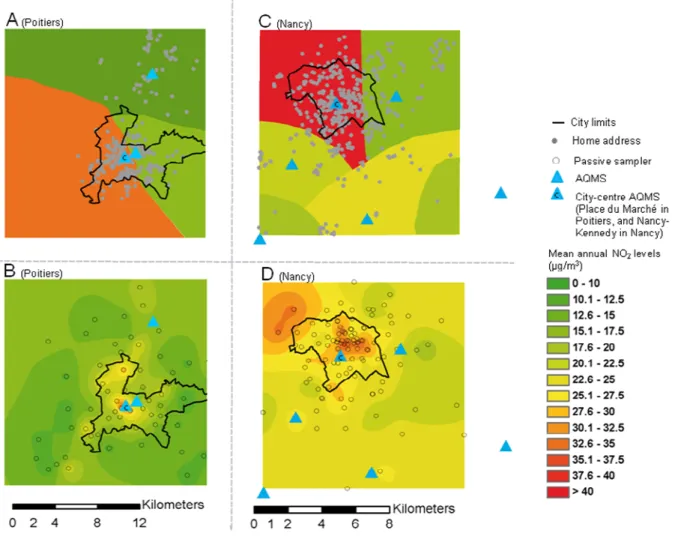
area and six in the Nancy area, Figures 1A and C), excluding those labeled as traffic (i.e.
located <5 m from a road with traffic levels of >10,000 vehicles/day (ADEME 2002)) or
industrial stations. For each woman i, hourly measures of NO2 concentration by the AQMS j
closest to her home address were averaged over each time-window considered (noted ∆t for
convenience), to obtain our exposure estimate .
Temporally adjusted geostatistical model (model 2)
NO2 measurement campaigns with a Palmes diffusive sampler (Palmes et al. 1976) were
conducted in the urban and peri-urban areas of both cities. The diffusive samplers were
located so as to give measurements of background pollution in each area (61 locations in the
Poitiers area, 98 locations in the Nancy area). The campaigns lasted 14 days (Poitiers) or 10 to
15 days (Nancy) and were repeated throughout the year to capture seasonal variations. Nine
campaigns were performed in 2005 in the Poitiers area and 10 were performed in 2002 in the
Nancy area (AIRLOR 2004; ATMO-PC 2007). In each area, for each passive sampler, the
10 passive sampler during campaigns was used to estimate mean annual concentration at each
measurement location. These estimated annual concentrations were smoothed over the whole
area with kriging techniques (Chilès and Delfiner 1999) on a 50x50 meter grid, with Isatis
Software (Géovariances, Fontainebleau; Figure 1B and D). This corresponded to our estimate
of , the mean NO2 concentration at the home address, for the year 2005 in Poitiers and
2002 in Nancy (spatial component of the model).
The estimated annual NO2 concentrations were then combined with time-specific
measurements from the permanent AQMS to capture temporal variations in concentrations.
This approach has previously been used in the context of LUR models (Slama et al. 2007).
The hourly NO2 measures of all AQMS from the area were averaged over each time-window
∆t considered
(Siall, ∆t) and also over the year in which the measurement campaign was performed (Sall, yearly).
The ratio Siall, ∆t / Sall, yearly was the temporal component of the model. The temporally adjusted
estimate of NO2 exposure E2i∆t for woman i was the product of the spatial and temporal
components, or
. [1]
Statistical analyses
Spatial and temporal variations in exposure
For each model, the relative contribution of spatial (or temporal) variations in exposure
contrasts was assessed by Pearson’s correlation coefficient between the exposure estimate and
its spatial (or temporal) component. We also carried out variance decomposition. The nearest
11
, [2]
With being the mean level of exposure of all women during the time-window ∆t, and Sij
the NO2 concentration at AQMS j averaged over the entire study period, so as to obtain a
spatial component dependent solely on the address of the woman. This
corresponded to our estimate of the spatial component of the AQMS model; (E1ij, ∆t – Sij)
corresponded to our estimate of the temporal component of the model. The TAG model was
log-transformed and expressed as
[3]
for the variance analysis. These analyses were restricted to women who did not change
address during pregnancy.
Comparison of the exposure estimates generated by each model
Exposure estimates for the two models were compared by Kruskal-Wallis rank tests and by
calculating correlation coefficients (r). The distributions of the exposures estimated by the
nearest AQMS model and by the TAG model were plotted either as a function of the AQMS
closest to woman’s home address, then excluding the AQMS located in the city-center. We
also assessed the concordance between the estimates generated by the two models, classified
into tertiles, by determining percentage concordance and the kappa coefficient (K).
Bland-Altman plots were used to estimate the magnitude of the systematic error between the two
exposure models (Bland and Altman 1986).
Exposure-response relationship
We studied the relationship between birthweight and NO2 exposure during each exposure
12 factors. Linear trend tests were performed with a categorical variable, the value of which
corresponded to the category-specific median NO2 concentration. The adjustment factors were
selected on the basis of a priori knowledge (Rothman et al. 2008). We adjusted for active and
passive smoking during the second trimester of pregnancy, because these factors were more
strongly associated with birthweight than exposures during the first trimester, the third
trimester or any of the three trimesters. We also adjusted for sex of the newborn, maternal
height (as a continuous variable), pre-pregnancy weight (broken stick model with a knot at 60
kg), birth order, maternal age at end of education, center, and trimester of pregnancy.
Statistical analyses were carried out with STATA statistical software (Stata SE 10.1, Stata
Corp, College Station, TX). Analyses were repeated for the three buffers considered (less than
13
Results
Population
Of the 1893 women from the cohort with a known offspring birthweight, 776 lived in the
study area, less than 5 km from an AQMS, during at least one trimester of pregnancy (431 and
158 women lived within 2 and 1 km of an AQMS, respectively). Mean birthweight was 3284
g (25, 50, 75th percentiles, 3005, 3310, 3620 g). The characteristics of the study population
are described in Table 1.
Exposure to air pollutants
Estimates of exposure to NO2 were higher in Nancy than in Poitiers, whatever the exposure
model and exposure window considered (Figure 1, Tables 1 and 2). The nearest AQMS model
estimate during pregnancy was more strongly correlated with the spatial component of the
TAG model (r=0.61, 0.68, 0.84, for the 5, 2, 1 km buffers, respectively) than with its temporal
component (r=0.35, 0.35, 0.45, respectively). For both models, exposure estimates throughout
pregnancy were subject to strong spatial variation (accounting for >90% of the variance of
exposure, Table 3). Temporal variations made a greater contribution to total variation when
we considered trimester-specific windows, but remained smaller than spatial variations for the
nearest AQMS model (72-84% for spatial variation and 20-25% for temporal variation),
whereas the contributions of the spatial and temporal variation components were similar for
the TAG model (43-61% for spatial variation and 44-57% for temporal variation, Table 3).
The buffer around the AQMS studied had no major effect on the relative contributions of
spatial and temporal components of variation.
The levels and range of NO2 concentrations estimated by the nearest AQMS model were
greater than those estimated by the TAG model (Table 2). Bland and Altman plots (See
14 increased with mean exposure estimates. This pattern was principally due to between-model
differences for women living in the city-centers (mean NO2 concentrations estimated by the
nearest AQMS model were higher and ranges were narrower than for the TAG model), rather
than in the peri-urban areas. Indeed, the exposure distributions for the two models became
more similar when city-center AQMS measurements were not taken into account (Figure 2).
All this indicates that the overestimation of NO2 exposure levels by the AQMS model with
respect to the TAG model mainly concerned the women who were also the most exposed with
the TAG model.
The correlation and concordance (K) between the two exposure models were fair (0.40 -0.74)
when we considered all the women living within 5 km of an AQMS (Table 2 and
Supplemental Material, Figure 2), but were stronger if we restricted the study population to
women living within 2 (0.37 -0.79) or 1 km (0.59 -0.87) of an AQMS. The correlation and
concordance between the two exposure models also differed between the areas
(Nancy/Poitiers) and between the city center and suburban areas (See Supplemental Material,
Figure 2).
Associations between air pollutants and fetal growth
The patterns of association with birthweight identified were similar for the two exposure
models, in terms of estimates of adjusted effects and confidence intervals (CI), although these
associations were stronger for the nearest AQMS model (Figure 3, and see Supplemental
Material, Table 1). The first and third trimesters of pregnancy corresponded to the exposure
windows most clearly associated with effects on birthweight, for both exposure models. For
women living less than 2 km from an AQMS, an increase of 10 µg/m3 in NO2 concentration
during the first trimester of pregnancy was associated with an adjusted change in mean
-15 128; 26 g) for the TAG model. Qualitatively similar results were obtained when exposure was
coded in tertiles (See Supplemental Material, Table 1). For the AQMS model, the parameter
quantifying the association between NO2 exposure and birthweight approached 0 as buffer
size increased. Similar results were obtained if no adjustment was made for the center (results
16
Discussion
Our study is one of the first to describe associations between NO2 exposure assessed with a
TAG model and birthweight, and to compare this model with the more commonly used
approach based on permanent AQMS. Models were compared in terms of both exposure
estimates and association with birthweight. The nearest AQMS model was influenced by the
location of monitors. Variations in exposure were mostly due to spatial rather than temporal
variations in both models, with temporal variation making a larger overall contribution to total
variation in the TAG model than in the nearest AQMS model. The concordance between NO2
exposures estimates with the two models was fair when the 5 km buffer was considered. This
concordance was stronger if the analysis was restricted to women living closer (<2 km, and
more clearly, <1 km) to an AQMS. When exposure was coded as a continuous term,
associations with birthweight for the TAG model were consistent with those obtained in
analyses based on exposure estimated from the nearest AQMS model, for the various buffers
around AQMS and exposure windows.
The TAG model is thought to have a better spatial resolution than the nearest AQMS model,
due to the use of data from fine measurement campaigns, with no loss of temporal resolution,
because TAG exposure estimates were seasonalized on the basis of AQMS measurements.
The stronger contribution of the spatial component in the nearest AQMS model than in the
TAG model may at first glance appear counterintuitive, as the AQMS model could be
considered to be essentially based on temporal variations. However, this finding may be
accounted for by the considerable variation of the concentrations obtained with different
AQMS, some of which (in the city center) were influenced by traffic, despite meeting the
criteria for background stations. This illustrates the extent to which the nearest AQMS
17 finer spatial resolution in studies with medium- or long-term exposure windows (3 to 9
months in our study). As passive samplers were located at background sites less affected by
traffic, the TAG approach led to a more purely background model than the AQMS approach.
The higher concentrations estimated by the nearest AQMS model than by the TAG model
(Table 2) may be accounted for by this feature. The TAG model may also smooth extreme
exposure values, leading to an underestimation of the role of spatial variation.
One possible limitation of the TAG model stems from the approach used to seasonalize this
model, in which we assumed that spatial differences in exposure remained constant over time.
This assumption was found to be reasonable for an LUR model developed in Rome (Porta et
al. 2009), but may not hold in other areas with different characteristics.
Several studies have evaluated the performance of AQMS for estimating exposure to air
pollutants (Marshall et al. 2008; Nerriere et al. 2005; Nethery et al. 2008; Sarnat et al. 2005).
The last three of these studies reported poor concordance between AQMS estimates and
personal monitoring data, which is not surprising because personal exposure is not expected
to strictly correspond to background levels of air pollution at the home address. Marshall et al.
(2008) reported correlations and Kappa coefficients for estimates from the nearest AQMS
model (within 10 km) and estimates stemming from either an LUR (r=0.61, K=0.42) or a
dispersion model (r=0.37, K=0.22). The concordance obtained with the LUR model was
similar to that observed in our study with the TAG model for a 5 km buffer around the
AQMS. However, Marshall’s study is not directly comparable with ours, because they used a
larger buffer zone (10 km) and because the LUR and dispersion models incorporate all local
sources of pollution, whereas our TAG model does not.
In this study, we focused on women living less than 5 km from an AQMS, whereas previous
18 km (5 miles) from a monitor (Basu et al. 2004; Brauer et al. 2008; Parker et al. 2005). Our
results indicate that the size of buffer around monitors considered has a major effect on the
concordance between models and the estimated association between NO2 concentration and
birthweight. Higher levels of concordance between the models were obtained if we focused
on women living within 2 km of a monitor, with concordance levels even higher if we limited
the analysis to women living within 1 km of a monitor. Associations between NO2 levels and
birthweight, although not statistically significant at the 5% level, tended to be stronger for the
2 km buffer around the AQMS than for the 5 km buffer (Figure 3). The findings were
sometimes less clear for women living within 1 km of an AQMS, and the confidence intervals
were slightly larger than for the 2 km buffer, probably because of the small number of
subjects. Previous studies (Hansen et al. 2008; Wilhelm and Ritz 2005) with buffers of
different sizes gave results similar to ours: the authors found stronger negative associations
between fetal growth and levels of exposure to carbon monoxide, PM10, SO2 and O3 during
pregnancy, as estimated from data from the nearest AQMS, for women living within 2 km of
a station than for those living up to 14 km away. The choice of the buffer size can probably be
seen as a trade-off between bias and variance: the use of smaller buffers decreases sample
size (increasing variance) but also probably decreases exposure misclassification (assuming
that exposure is generally less well assessed for subjects living further away from an AQMS).
However, selection bias may also contribute to the increase in the absolute value of the
regression parameter quantifying the association between exposure and birthweight when
smaller buffers are considered. Indeed, for associations with third-trimester exposure (but less
clearly for first-trimester exposure), the absolute value of the regression parameter also tended
to increase as buffer size decreased for the TAG model. This is unlikely to be due to
variations in exposure misclassification and might instead be attributed to differences in the
19 Most previous studies considering the effects of NO2, have reported larger decreases in
birthweight for exposure in the first and third trimesters of pregnancy (Bell et al. 2007;
Gouveia et al. 2004; Ha et al. 2001; Liu et al. 2007; Mannes et al. 2005; Salam et al. 2005)
than for exposure in the second trimester or over the entire pregnancy (Ha et al. 2001; Lee et
al. 2003; Mannes et al. 2005). A similar pattern was observed in our study. A discussion of
the biological relevance of the exposure window or the underlying mechanisms is beyond the
scope of this article. Several potential mechanisms by which air pollution may affect fetal
growth have been proposed (Kannan et al. 2006; Ritz and Wilhelm 2008; Slama et al. 2008),
but none of these mechanisms has been validated.
It is generally difficult to predict the impact of an error in an exposure variable in terms of the
potential for bias in the exposure-response relationship (Jurek et al. 2008). However, in the
specific case of a Berkson-type error, the power of the study is reduced and confidence
intervals are widened, but no bias in linear regression coefficients is expected (Armstrong
2008; Zeger et al. 2000). Berkson-type error (Armstrong 2008) may occur when the exposure
is measured at the population level and individual exposures levels vary because of
differences in the time windows of exposure or time-activity patterns. The measurement error
for the nearest AQMS approach would be expected to have a Berkson-type component,
because the same proxy exposure is used for all women living in a circular area around a
given monitor. The observation that exposure estimates for the nearest AQMS model were at
least as strongly associated with birthweight as those for the TAG model is consistent with the
nearest AQMS model being subject principally to Berkson-type error. Therefore, assuming
that the observed association with birthweight was real, exposure misclassification seemed to
have little impact on the dose-response relationship. If we accept that the TAG model cannot
be seen as a gold standard, exposure mismeasurement seemed to affect both models in similar
20 between NO2 exposure and fetal growth when they used an AQMS-based approach, but no
association when they used a LUR model. They considered women living up to 10 km away
from an AQMS, and the AQMS-based model corresponded to an inverse-distance weighting
21
Conclusion
Our study indicates that models of exposure to background NO2 concentrations based on data
from the nearest AQMS may entail large errors in estimated exposure, but that in some
instances these errors have little impact on the exposure-birthweight relationship. The
amplitude of exposure misclassification in AQMS-based models and of the resulting bias may
be limited by restricting the size of the study area around each AQMS considered. Full
quantification of the exposure error for each model would require a consideration of the
temporal and spatial activities of each subject. Our study cannot be interpreted as providing
clear evidence that the nearest AQMS approach yields unbiased estimates of the association
between NO2 concentrations and fetal growth. This question requires further consideration in
other cohorts and in other countries, in which the sitting of permanent monitors may follow
22
References
ADEME. 2002. Classification and Criteria for Setting Up Air-Quality Monitoring Stations [in
French]. Paris ADEME Éditions.
AIRLOR. 2004. Etude de la distribution du dioxyde d'azote par la méthode des tubes passifs
sur l'agglomération Nancéienne été-hiver 2002 [in French]. Available:
http://www.atmolor.org/site/medias/_telechargements/_etudes/_campagnes/airlor/2002/Rappo
rt_CUGN_2002_sans_annexes.pdf [accessed 22 September 2009].
Armstrong B. 2008. Measurement error: Consequences and design issues. In: Environmental
epidemiology: study methods and application (Baker D, Nieuwenhuijsen M, eds). Oxford ;
New York: Oxford University Press, 93-112.
ATMO-PC. 2007. Vent d'Ouest. Bulletin d'information sur la qualité de l'air en
Poitou-Charentes. [in French]. Available:
http://www.atmo-poitou-charentes.org/IMG/swf/ventdouest17_86.swf [accessed 22 September 2009].
Basu R, Woodruff TJ, Parker JD, Saulnier L, Schoendorf KC. 2004. Comparing exposure
metrics in the relationship between PM2.5 and birth weight in California. J Expo Anal
Environ Epidemiol 14(5):391-396.
Bell ML, Ebisu K, Belanger K. 2007. Ambient air pollution and low birth weight in
Connecticut and Massachusetts. Environ Health Perspect 115(7):1118-1124.
Bland JM, Altman DG. 1986. Statistical methods for assessing agreement between two
methods of clinical measurement. Lancet 1(8476):307-310.
Brauer M, Lencar C, Tamburic L, Koehoorn M, Demers P, Karr C. 2008. A cohort study of
traffic-related air pollution impacts on birth outcomes. Environ Health Perspect
116(5):680-686.
Chilès JP, Delfiner P. 1999. Geostatistics: modelling spatial uncertainty. Wiley Series in
23 Drouillet P, Forhan A, De Lauzon-Guillain B, Thiebaugeorges O, Goua V, Magnin G, et al.
2008. Maternal fatty acid intake and fetal growth: evidence for an association in overweight
women. The 'EDEN mother-child' cohort (study of pre- and early postnatal determinants of
the child's development and health). Br J Nutr:1-9.
Gouveia N, Bremner SA, Novaes HM. 2004. Association between ambient air pollution and
birth weight in Sao Paulo, Brazil. J Epidemiol Community Health 58(1):11-17.
Ha EH, Hong YC, Lee BE, Woo BH, Schwartz J, Christiani DC. 2001. Is air pollution a risk
factor for low birth weight in Seoul? Epidemiology 12(6):643-648.
Hansen CA, Barnett AG, Pritchard G. 2008. The effect of ambient air pollution during early
pregnancy on fetal ultrasonic measurements during mid-pregnancy. Environ Health Perspect
116(3):362-369.
Jurek AM, Greenland S, Maldonado G. 2008. How far from non-differential does exposure or
disease misclassification have to be to bias measures of association away from the null?
International Journal of Epidemiology 37(2):382-385.
Kannan S, Misra DP, Dvonch JT, Krishnakumar A. 2006. Exposures to airborne particulate
matter and adverse perinatal outcomes: a biologically plausible mechanistic framework for
exploring potential effect modification by nutrition. Environ Health Perspect
114(11):1636-1642.
Lebret E, Briggs D, van Reeuwijk H, Fischer P, Smallbone K, Harssema H, et al. 2000. Small
area variations in ambient NO2 concentrations in four European areas. Atmos Environ
34(2):177-185.
Lee BE, Ha EH, Park HS, Kim YJ, Hong YC, Kim H, et al. 2003. Exposure to air pollution
during different gestational phases contributes to risks of low birth weight. Hum Reprod
18(3):638-643.
24 to ambient air pollutants during pregnancy and fetal growth restriction. J Expo Sci Environ
Epidemiol 17(5):426-432.
Mannes T, Jalaludin B, Morgan G, Lincoln D, Sheppeard V, Corbett S. 2005. Impact of
ambient air pollution on birth weight in Sydney, Australia. Occup Environ Med
62(8):524-530.
Marshall JD, Nethery E, Brauer M. 2008. Within-urban variability in ambient air pollution:
Comparison of estimation methods. Atmos Environ 42(6):1359-1369.
Miller KA, Siscovick DS, Sheppard L, Shepherd K, Sullivan JH, Anderson GL, et al. 2007.
Long-term exposure to air pollution and incidence of cardiovascular events in women. N Engl
J Med 356(5):447-458.
Nerriere E, Zmirou-Navier D, Blanchard O, Momas I, Ladner J, Le Moullec Y, et al. 2005.
Can we use fixed ambient air monitors to estimate population long-term exposure to air
pollutants? The case of spatial variability in the Genotox ER study. Environ Res 97(1):32-42.
Nethery E, Leckie SE, Teschke K, Brauer M. 2008. From measures to models: an evaluation
of air pollution exposure assessment for epidemiological studies of pregnant women. Occup
Environ Med 65(9):579-586.
Palmes ED, Gunnison AF, DiMattio J, Tomczyk C. 1976. Personal sampler for nitrogen
dioxide. Am Ind Hyg Assoc J 37(10):570-577.
Parker JD, Woodruff TJ, Basu R, Schoendorf KC. 2005. Air pollution and birth weight
among term infants in California. Pediatrics 115(1):121-128.
Porta D, Cesaroni G, Badaloni C, Stafoggia M, Meliefste C, Forastiere F, et al. 2009.
Nitrogen dioxide spatial variability in Rome (Italy): an application of the LUR model over a
decade. In: 21th Annual Conference of the
International-Society-for-Environmental-Epidemiology. Dublin, Ireland, In press.
25 issues in an emerging field. Basic Clin Pharmacol Toxicol 102(2):182-190.
Rothman KJ, Greenland S, Last TL. 2008. Modern epidemiology. 3rd ed. Philadelphia:
Wolters Kluwer | Lippincott Williams & Wilkins.
Salam MT, Millstein J, Li YF, Lurmann FW, Margolis HG, Gilliland FD. 2005. Birth
outcomes and prenatal exposure to ozone, carbon monoxide, and particulate matter: results
from the Children's Health Study. Environ Health Perspect 113(11):1638-1644.
Sarnat JA, Brown KW, Schwartz J, Coull BA, Koutrakis P. 2005. Ambient gas concentrations
and personal particulate matter exposures - Implications for studying the health effects of
particles. Epidemiology 16(3):385-395.
Slama R, Darrow L, Parker J, Woodruff TJ, Strickland M, Nieuwenhuijsen M, et al. 2008.
Meeting report: atmospheric pollution and human reproduction. Environ Health Perspect
116(6):791-798.
Slama R, Morgenstern V, Cyrys J, Zutavern A, Herbarth O, Wichmann HE, et al. 2007.
Traffic-related atmospheric pollutants levels during pregnancy and offspring's term birth
weight: a study relying on a land-use regression exposure model. Environ Health Perspect
115(9):1283-1292.
Slama R, Thiebaugeorges O, Goua V, Aussel L, Sacco P, Bohet A, et al. 2009. Maternal
Personal Exposure to Airborne Benzene and Intra-Uterine Growth. Environ Health Perspect
117(8):1313-1321.
Van Roosbroeck S, Hoek G, Meliefste K, Janssen NA, Brunekreef B. 2008. Validity of
residential traffic intensity as an estimate of long-term personal exposure to traffic-related air
pollution among adults. Environ Sci Technol 42(4):1337-1344.
Wilhelm M, Ritz B. 2003. Residential proximity to traffic and adverse birth outcomes in Los
Angeles county, California, 1994-1996. Environ Health Perspect 111(2):207-216.
26 birth outcomes in Los Angeles County, California, USA. Environ Health Perspect
113(9):1212-1221.
Yazbeck C, Thiebaugeorges O, Moreau T, Goua V, Debotte G, Sahuquillo J, et al. 2009.
Maternal Blood Levels and the Risk of Pregnancy-Induced Hypertension: The EDEN Cohort
Study. Environ Health Perspect 117(10):1526-1530.
Zeger SL, Thomas D, Dominici F, Samet JM, Schwartz J, Dockery D, et al. 2000. Exposure
measurement error in time-series studies of air pollution: concepts and consequences. Environ
27
TABLES
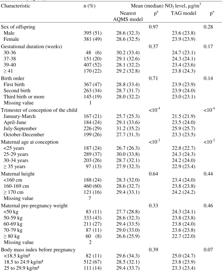
Table 1: Characteristics of the participants and their association with NO2 levels averaged
during pregnancy (n=776 women living less than 5 km away from an air quality monitoring station (AQMS)).
Characteristic n (%) Mean (median) NO2 level, µg/m3
Nearest AQMS model p a TAG model pa Sex of offspring Male Female 395 (51) 381 (49) 28.6 (32.3) 28.6 (32.5) 0.97 23.6 (23.8) 23.9 (23.9) 0.28
Gestational duration (weeks) 30-36 37-38 39-40 ≥ 41 48 (6) 151 (20) 407 (52) 170 (22) 30.2 (33.4) 29.1 (32.6) 28.1 (32.2) 29.2 (32.8) 0.37 24.7 (23.1) 24.3 (24.1) 23.4 (23.6) 23.8 (24.3) 0.17 Birth order First birth Second birth Third birth or more
Missing value 367 (47) 263 (34) 145 (19) 1 28.8 (33.4) 28.7 (31.7) 28.0 (32.2) 0.71 23.9 (23.9) 23.9 (24.0) 23.0 (23.1) 0.14
Trimester of conception of the child January-March April-June July-September October-December 167 (21) 184 (24) 226 (29) 199 (26) 25.7 (25.3) 29.1 (33.6) 31.2 (35.2) 27.7 (31.3) <10-4 21.5 (21.9) 23.5 (24.0) 25.9 (25.7) 23.3 (23.5) <10-4
Maternal age at conception <25 years 25-29 years 30-34 years ≥ 35 years 187 (24) 289 (37) 203 (26) 97 (13) 26.7 (26.3) 30.0 (33.8) 28.7 (32.1) 27.9 (32.3) <10-2 22.8 (22.7) 24.3 (24.3) 24.2 (24.0) 22.9 (23.4) <10-2 Maternal height <160 cm 160-169 cm ≥ 170 cm Missing value 188 (24) 460 (60) 121 (16) 7 28.3 (32.0) 28.6 (32.7) 29.4 (33.1) 0.64 23.4 (24.0) 23.8 (23.8) 24.2 (24.2) 0.44
Maternal pre-pregnancy weight <50 kg 50-59 kg 60-69 kg 70-79 kg ≥ 80 kg Missing value 83 (11) 333 (43) 211 (27) 87 (11) 60 (8) 2 27.7 (28.8) 28.6 (32.3) 29.4 (33.5) 29.0 (33.0) 26.6 (25.9) 0.33 24.3 (24.1) 23.8 (23.8) 23.8 (24.0) 23.6 (23.8) 22.7 (22.0) 0.46
Body mass index before pregnancy <18.5 kg/m² 18.5 to 24.9 kg/m² 25 to 29.9 kg/m² 82 (11) 512 (67) 111 (14) 29.6 (34.3) 28.5 (32.1) 29.4 (33.7) 0.39 25.0 (24.7) 23.8 (23.9) 23.3 (23.4) 0.07
28 ≥30 kg/m² Missing value 62 (8) 9 27.1 (30.6) 23.0 (22.4) Center Poitiers Nancy 316 (41) 460 (59) 24.9 (18.8) 31.2 (34.4) <10-4 20.3 (19.2) 26.1 (25.7) <10-4
Maternal age at end of education ≤16 years 17-18 years 19-20 years 21-22 years 23-24 years ≥ 25 years 52 (7) 104 (13) 124 (16) 165 (21) 174 (22) 157 (20) 29.6 (33.1) 27.0 (29.6) 27.1 (29.1) 27.9 (30.0) 29.3 (33.1) 30.6 (34.5) 0.02 24.0 (23.6) 22.2 (21.9) 23.2 (23.0) 23.3 (23.5) 24.5 (24.6) 24.7 (24.6) <10-3
Maternal active smoking (2nd trimester) No Yes Missing value 641 (83) 133 (17) 2 28.8 (32.7) 28.1 (32.0) 0.45 23.8 (24.0) 23.3 (22.8) 0.30
Maternal passive smoking (2nd trimester) No Yes Missing value 507 (66) 264 (34) 5 28.5 (32.1) 29.0 (33.3) 0.48 23.7 (23.9) 23.9 (23.6) 0.53
AQMS: Air Quality Monitoring Station, TAG: Temporally adjusted geostatistical model
a p-value comparing model specific exposure estimates between categories (Student test
for dichotomous variables) or among categories (Fischer’s analysis of variance for variables with >2 categories). Tests were performed without including missing data as a separate category.
29 nearest air quality monitoring station (AQMS) model and the temporally adjusted geostatistical (TAG) model, for various exposure windows and buffer sizes considered around AQMS.
Nearest AQMS model (5km
buffer) Between-model agreement
TAG model (5km buffer)
Distance a <5km Distance a <2km Distance a <1km
Area exposure window n NO2 levels n NO2 levels pb n r c K n r c K n r c K Both areas 1st trimester 770 28.8 ± 10.8 (11.3, 30.1, 43.6) 773 23.7 ± 6.2 (13.6, 23.0, 34.6) 10 -4 767 0.67 61 0.41 429 0.70 62 0.43 158 0.83 75 0.63 2nd trimester 771 29.0 ± 10.9 (11.5, 30.0, 43.9) 770 24.1 ± 6.5 (13.6, 23.6, 34.4) 10 -4 766 0.69 60 0.40 426 0.72 58 0.37 156 0.82 73 0.60 3rd trimester 770 28.1 ± 11.1 (10.4, 29.4, 44.2) 772 23.3 ± 6.8 (12.5, 22.8, 34.7) 10 -4 767 0.74 63 0.44 428 0.79 68 0.52 155 0.87 79 0.68 Whole pregnancy 776 28.6 ± 10.0 (13.3, 32.4, 41.8) 770 23.7 ± 5.0 (16.1, 23.8, 32.3) 10 -4 770 0.65 63 0.44 428 0.70 64 0.46 157 0.85 73 0.59 Poitiers area 1st trimester 310 25.6 ± 11.9 ( 9.3, 21.6, 43.0) 316 20.9 ± 6.3 (12.0, 20.4, 35.8) <10-3 310 0.61 59 0.38 181 0.65 57 0.36 75 0.89 83 0.74 2nd trimester 311 25.2 ± 11.6 (10.1, 22.2, 42.7) 315 20.4 ± 6.1 (11.8, 19.9, 32.0) 10-4 311 0.61 56 0.34 179 0.65 57 0.36 74 0.83 63 0.45 3rd trimester 310 23.9 ± 11.3 ( 8.5, 21.7, 42.0) 315 19.5 ± 6.3 (11.5, 19.0, 30.8) 10-4 310 0.66 62 0.43 179 0.72 67 0.51 73 0.86 78 0.67 Whole pregnancy 316 24.9 ± 10.6 (12.4, 18.8, 40.5) 316 20.3 ± 4.7 (14.7, 19.2, 30.0) 0.12 316 0.55 56 0.34 181 0.62 58 0.37 75 0.87 68 0.52 Nancy area 1st trimester 460 31.0 ± 9.5 (13.6, 31.3, 44.1) 457 25.7 ± 5.2 (17.9, 25.5, 34.6) 10-4 457 0.67 55 0.32 248 0.69 58 0.36 83 0.72 59 0.39 2nd trimester 460 31.6 ± 9.6 (14.1, 32.0, 44.4) 455 26.7 ± 5.5 (18.5, 26.6, 35.6) 10-4 455 0.70 58 0.37 247 0.73 65 0.48 82 0.74 66 0.49 3rd trimester 460 30.9 ± 10.0 (13.5, 31.4, 45.0) 457 26.0 ± 5.8 (17.5, 25.7, 36.2) 10-4 457 0.74 61 0.41 249 0.78 67 0.51 82 0.82 76 0.63 Whole pregnancy 460 31.2 ± 8.7 (16.9, 34.4, 42.4) 454 26.1 ± 3.7 (20.8, 25.7, 32.8) 10 -4 454 0.66 64 0.46 247 0.69 64 0.47 82 0.66 71 0.56
r: Pearson correlation coefficient, c: concordance percentage (based on NO2 levels categorized in tertiles), K: Kappa coefficient (based on NO2 levels categorized in
tertiles).
a: Maximal distance between home address and the nearest AQMS (buffer size).
30
Table 3: Variance component (%) of NO2 exposure levels estimated by the nearest air quality monitoring station (AQMS) model and by the temporally
adjusted geostatistical (TAG) model for various exposure windows and buffer sizes considered around AQMS.
Distance <5km (n=681) Distance <2km (n=383) Distance <1km (n=146)
Nearest AQMS model
TAG model Nearest AQMS
model
TAG model Nearest AQMS
model
TAG model Exposure
window
Spatial Temporal Spatial Temporal Spatial Temporal Spatial Temporal Spatial Temporal Spatial Temporal
1st trimester 82 21 61 52 79 22 55 57 84 25 56 49
2nd trimester 82 20 55 46 79 21 53 52 83 21 58 44
3rd trimester 78 21 47 46 76 21 43 52 80 24 52 48
Pregnancy 95 7 92 14 91 8 92 17 97 9 92 13
31
Figure legends
Figure 1: Mean annual NO2 levels estimated by the nearest air quality monitoring station
(AQMS) model in Poitiers (A) and Nancy areas (C), and by the temporally adjusted
32 pregnancy as estimated by the nearest air quality monitoring station (AQMS) model and by the
temporally adjusted geostatistical (TAG) model, according to the AQMS closest to the
residential address. Population restricted to 735 women living less than 5 km away from an
AQMS without change of assigned station during pregnancy.
a: Exposures were estimated taking into account all AQMS.
b: Exposures were estimated taking into account all AQMS except K and M (city-center
stations); for subjects initially assigned to one of these stations, the closest station has been replaced by the second AQMS nearest to the home address located outside the city center and less than 5 km away from the home address, if any.
c: Exposures were estimated taking into account all AQMS except K and M; all women for
whom K or M is the closest station have been excluded from the analysis.
T: Tomblaine, K: Nancy-Kennedy, B: Nancy-Brabois, F: Fléville, S: St Nicolas de Port, N: Neuves-Maison, L: Les couronneries, M: Place du marché, C: Chasseneuil. Stations located in the peri-urban area. Letters identifying stations located in the city center are underlined.
33 pregnancy, as a function of the size of the buffer considered around each air quality monitoring
station (AQMS). The error bars indicate the 95% CIs.
a adjusted for maternal age at conception, gestational age at delivery (linear and quadratic terms),
sex of newborn, maternal height (continuous variable), pre-pregnancy weight (broken stick model with a knot at 60 kg), birth order, center, trimester of conception, maternal age at end of education, active smoking during the second trimester of pregnancy (binary variable), passive smoking during the second trimester of pregnancy.