HAL Id: hal-03260974
https://hal.uca.fr/hal-03260974
Submitted on 15 Jun 2021
HAL is a multi-disciplinary open access archive for the deposit and dissemination of sci-entific research documents, whether they are pub-lished or not. The documents may come from teaching and research institutions in France or abroad, or from public or private research centers.
L’archive ouverte pluridisciplinaire HAL, est destinée au dépôt et à la diffusion de documents scientifiques de niveau recherche, publiés ou non, émanant des établissements d’enseignement et de recherche français ou étrangers, des laboratoires publics ou privés.
Migration, remittances and poverty in Ecuador *
Simone Bertoli, Francesca Marchetta
To cite this version:
Simone Bertoli, Francesca Marchetta. Migration, remittances and poverty in Ecuador *. The Journal of Development Studies, Taylor & Francis (Routledge), 2013, 50 (8), pp.1067-1089. �10.1080/00220388.2014.919382�. �hal-03260974�
Migration, remittances and poverty in Ecuador
∗
Simone Bertoli
aand Francesca Marchetta
ba
CERDI†, University of Auvergne and CNRS
bCERDI‡, University of Auvergne
Abstract
We analyse the influence of the recent wave of migration on the incidence of poverty among stayers in Ecuador. We draw our data from a survey that provides detailed information on migrants. The analysis reveals a significant negative effect of migration on poverty among migrant households. This effect is substantially smaller than the one that we find focusing on recipient households. We explore the factors that account for this divergence. Our analysis entails that the existing empirical evidence on the relationship between remittances and poverty needs not to be informative about the size of the direct poverty-reduction potential of migration.
Keywords: remittances; household-level data; poverty; propensity score matching. JEL codes: F22; O15; I32.
∗The authors are grateful the editor Richard Palmer-Jones and to two anonymous referees for their care-ful reading of our paper, and to Sascha Becker, Arjun Bedi, Simon Cueva, Francesca Francavilla, Mihails Hazans, Jos Hidalgo Pallares, Mauricio Len, Jeannette Sanchez and to the participants in the TOM Confer-ence on Transnationality of Migrants, First ConferConfer-ence on Migration and Development, INFER ConferConfer-ence, 30th Journes de Microconomie Applique, 62nd AFSE Annual Meeting and in seminar presentations at the International Institute of Social Studies and the IAB for their comments; they also gratefully acknowledge the contribution of Marco Quinteros, the former director of the INEC, who allowed them to get access to the data; This research was supported by the Agence Nationale de la Recherche of the French government through the program Investissements d’avenir (ANR-10-LABX-14-01) and by the FERDI (Fondation pour les tudes et recherches sur le dveloppement international). The usual disclaimers apply.
†CERDI, University of Auvergne, Bd. F. Mitterrand, 65, 63000, Clermont-Ferrand, France; email: [email protected], phone: +33 473 177514, fax: +33 473 177428 (corresponding author).
‡CERDI, University of Auvergne, Bd. F. Mitterrand, 65, 63000, Clermont-Ferrand, France; email: [email protected].
1
Introduction
What is the influence exerted by international migration on the poverty status of the house-hold members left behind? Providing an answer to this question requires comparing the observed incidence of poverty for migrant households1 with the one prevailing in a
counter-factual scenario where all household members stay at home. The economic literature has been mostly focusing on a related but distinct research question, namely the analysis of the relationship between the receipt of migrants’ remittances and the incidence of poverty among stayers (Gustafsson and Makonnen, 1993; Leliveld, 1997; Acosta et al., 2006, 2008; Yang and Martinez, 2007; Lokshin et al., 2010; Adams and Cuecuecha, 2013).2 Still, the “growing view
in the literature that remittances can have a positive impact on economic development by reducing poverty” (Adams and Cuecuecha, 2013, p. 38) needs not to be informative about the size of the direct poverty-reduction potential of international migration. This is due to the analytical choice of some of the papers in the literature to analyse the effects of remit-tances while taking migration decisions as given, and to the non coincidence of the group of migrant and of recipient households.
Specifically, Gustafsson and Makonnen (1993), Leliveld (1997) and Adams and Cue-cuecha (2013) compare the observed incidence of poverty among recipient households with the incidence that would have prevailed in a hypothetical scenario with no remittances but with an unchanged household composition. Other papers analyse a no remittances and no migration counterfactual, and the choice to focus on the relationship between the receipt of remittances and the incidence of poverty among stayers appears to be data-driven as the data either do not allow to identify migrant households (Acosta et al., 2006, 2008) or they just provide information on the migrants that send remittances (Lokshin et al., 2010). The econometric evidence provided by these papers is informative about the poverty-reduction potential of international migration only if the receipt of remittances represents a good proxy for the unknown migration status of the household, but there are theoretical and empirical reasons why this is unlikely to be the case.
From a theoretical perspective, the so-called new economics of labor migration portrays migration as a joint decision of the migrant and of some group of stayers, where remittances ensure that the monetary returns from migration are shared with the non-migrants that contributed to finance the cost of the move. This group can extend beyond the household of origin of the migrant, so that some recipient households are not migrant households.
Similarly, not all migrant households are also recipient households,3 as the migrant might be unable or unwilling to abide to the “implicit contractual arrangement” she had agreed upon with the stayers (Stark and Bloom, 1985). For instance, migrants could experience spells of unemployment that prevent them from sending remittances, or they might deliberately decide not to transfer any money back home. The partial, and possibly limited, overlap between the groups of recipient and migrant households suggests to be wary of interpreting the available empirical evidence in the literature as being informative about the direct effect of international migration on poverty at origin. This effect depends on (i ) the change in total household income from domestic sources due to migration, (ii ) the variation in the number of household members residing at origin due to migration, and (iii ) the remittances sent back by the migrants.
Our paper analyses the effect of migration upon the incidence of income poverty among stayers in Ecuador, a country that experienced an unprecedented wave of international mi-gration induced by a severe economic crisis at the end of the 1990s. The poverty headcount rose by an estimated 2 million people between the mid- and the late-1990s (Parandekar et al., 2002) in a country with a population of 12.7 million. More than half a million Ecuadori-ans left the country within a few years’ time, mostly heading toward Spain and the US. The sorting of Ecuadorian migrants across destination and their pattern of selection on education were shaped by the combined effect of the crisis-induced liquidity constraints and of the high migration costs that Ecuadorian would-be migrants faced, which were partly policy-induced (Bertoli et al., 2011). Specifically, most of the recent migrants opted for Spain, where they enjoyed substantially lower income gains than in the US but where a bilateral visa waiver that had been granted since 1963 reduced the monetary costs of migration (Bertoli et al., 2013). Survey data collected in Spain reveal that the cost of migrating from Ecuador amounted on average to $1,800 (Bertoli et al., 2011); although this figure stands substantially below the estimated $7,000-$9,000 of attempting to migrate illegally to the US (Jokisch and Pribilsky, 2002), it still hindered both the participation of poor households to this migration wave and its ensuing influence on poverty at origin.
We draw the data for our analysis from the the Encuesta Nacional de Empleo, Desem-pleo y SubemDesem-pleo, ENEMDU, conducted by the INEC in December 2005. This labor market survey allows us to derive income-based definitions of poverty and it provides detailed in-formation on migrant members, including the year of migration, age, gender, education and
the amount of remittances sent over the previous 12 months. The availability of rich data on migrants represents a key value added of this survey, as our analysis exploits the informa-tion on the timing of the various migrainforma-tion episodes and the informainforma-tion on the individual characteristics of the migrants.
Specifically, the ability to identify migrant and not just recipient households allows us to directly analyse the relationship between international migration and poverty, and to compare our results with the ones that we obtain when we follow the more standard approach in the literature, which relies on the receipt of remittances as a proxy for the unobserved migration status of the household.4 Furthermore, the information on the timing of the
migration episodes allows us to define the treatment of interest as having sent at least one member abroad after 1998, the year that marks the start of the Ecuadorian crisis (Beckerman and Cort´es-Douglas, 2002; J´acome, 2004). This allows us to greatly reduce the heterogeneity of the influence on poverty that would arise if the group of treated households was based on migration episodes that are more distant in time, and it also reduces the strength of the effects of migration on the supply (Mishra, 2007) or on the demand side (Woodruff and Zenteno, 2007; Wahba and Zenou, 2012; Marchetta, 2012) of the labor market at origin that can indirectly influence non-migrants.
We resort to propensity score matching, PSM, to identify the effect of migration on poverty, as we lack a credible instrument for migration, and as this estimation technique does not require to introduce assumptions on the functional form of the relationship between household characteristics, migration and poverty. This estimation approach has been recently applied to the analysis of the effects of migration and remittances by, inter alia, Cox-Edwards and Rodr´ıguez-Oreggia (2009), Acosta (2011) and Jimenez-Soto and Brown (2012), although we acknowledge that the debate around its ability to produce unbiased estimates is still open (Dehejia, 2005; Smith and Todd, 2005a,b; Peikes et al., 2008). This is why we test the sensitivity of our estimates to possible departures from the identifying assumption following Rosenbaum (2002) and Becker and Caliendo (2007).
Our empirical analysis reveals that the recent Ecuadorian migration reduced the incidence of poverty among migrant households by an estimated 17.4-20.8 percent. This effect is statistically significant, although sensitive to possible violations of the identifying assumption of selection on observables.
from the questions related to migrants, as the income section of the questionnaire provides information related to the receipt of remittances from abroad over the month before the survey. When, as the literature does, we focus on recipient households, we find sharply different results, as the treatment is estimated to induce a decline in poverty by 57.2-59.2 percent. These estimates, which are in line with those obtained by Acosta et al. (2008) with data drawn from the 2004 round of the ENEMDU, entail that the poverty-reduction potential of international migration cannot, in the case of Ecuador, be inferred from the existing econometric evidence on the relationship between the receipt of remittances and poverty, and our paper explores the factors that can account for such a divergence in the results.
This paper is closely related to four different strands of literature. First, it draws on the papers that analyse the impact of migration and remittances on poverty at origin with household-level data (Yang and Martinez, 2007; Acosta et al., 2006, 2008; Lokshin et al., 2010; de la Fuente, 2010; Jimenez-Soto and Brown, 2012; Adams and Cuecuecha, 2013) and that estimate counterfactual domestic earnings for the migrants (Adams, 1989; Barham and Boucher, 1998). Second, it is related to the papers that analyse the determinants of migrants’ selection (Chiquiar and Hanson, 2005; McKenzie and Rapoport, 2010; Fern´ andez-Huertas Moraga, 2011, 2013). Third, it is connected to the vast literature on PSM originating from the seminal contribution by Rosenbaum and Rubin (1983), and in particular to the papers that deal with the use of sampling weights (Fr¨olich, 2007; Zanutto, 2006) and with departures from the identifying assumptions (Becker and Caliendo, 2007; Ichino et al., 2008; Nannicini, 2007). Fourth, this paper contributes to the strand of literature analyzing the determinants and the effects of the recent wave of Ecuadorian migration (Beckerman and Cort´es-Douglas, 2002; Jokisch and Pribilsky, 2002; J´acome, 2004; Gray, 2009; Calero et al., 2009; Bertoli, 2010; Bertoli et al., 2011, 2013).
The rest of the paper is structured as follows: Section 2 briefly describes the PSM tech-nique, and Section 3 discusses its implementation to the analysis of the effect of migration on poverty. The data source and the descriptive statistics are presented in Section 4. Section 5 presents the estimates and it explores the difference between the results obtained when focusing on migrant or on recipient households, and Section 6 concludes.
2
Propensity score matching
Households can be either subject to a treatment, zi = 1, or not, zi = 0, with T (U ) denoting
the subsample of treated (untreated) units. Let yi1 be the value of the outcome variable
when zi = 1, and let yi0 represent its value when zi = 0. The observed value of the outcome
variable yi is related to its potential outcomes by the observation rule:
yi = ziyi1+ (1 − zi)yi0
The treatment effect on the unit i is defined as τi = yi1− yi0. The average treatment
effect on the treated, ATET, is defined as:
ET(τi|zi = 1) = ET(yi1|zi = 1) − ET(yi0|zi = 1) (1)
where ET denotes the average on treated units only. The observational rule for yi
pre-cludes the estimation of the ATET, as yi0 is not observed when zi = 1. In a experimental
setting, we have that EU(yi0|zi = 0) = ET(yi0|zi = 1), so that observed outcomes for the
untreated units can substitute for the unobserved outcomes y0 for treated units. With
non-experimental data, this does not hold true because the assignment to the treatment can be influenced by a vector x of covariates that also exert an influence on y.
Assume that the vector x includes all covariates that have a simultaneous influence on the treatment and on the outcome, so that the potential outcome y0 is independent from z
conditional upon x. Formally:
y0 ⊥⊥ z|x (2)
where the symbol ⊥⊥ denotes statistical independence. Let f (x) represent the probability of assignment to treatment, which is also called the propensity score. The seminal contribu-tion by Rosenbaum and Rubin (1983) demonstrates that if f (x) ∈ (0, 1] and (2) holds, then we also have that:
y0 ⊥⊥ z|f (x) (3)
The outcome y0 is independent from the assignment to treatment z conditional upon
f (x), as f (x) represents a balancing score that ensures that x ⊥⊥ z|f (x) (Rosenbaum and Rubin, 1983). This, in turn, implies that the expected value of the unobserved outcome y0
for treated units conditional upon f (x) coincides with the expected value of the observed outcome y0 for untreated units:
Hence, the ATET can be estimated through an iterative averaging procedure: c ET(τi|zi = 1) = Z 1 0 h ET(yi1|zi = 1, f (x) = p) − EU(yi0|zi = 0, f (x) = p) i g(p)dp (4)
where g(p) denotes the distribution of the propensity score over the subsample T .
3
Implementation
We discuss here the key steps of the implementation of PSM to the analysis of the effect of migration on poverty for Ecuadorian households.5 The treatment z
i is represented by having
a household member who migrated, while the outcome yi is given by the income poverty
status.
3.1
Selection of the covariates
The first step is related to the identification of the variables that belong to x, as this vector has to include only variables that have a simultaneous influence on the probability to have a migrant member and upon the poverty status of the household. Variables that only have an impact on the probability to migrate should not be included, as the objective of the estimation of the propensity score is not to maximize the fit of the model (Caliendo and Kopeinig, 2008). The inclusion in x of variables that influence exclusively the treatment would actually reduce the ability of the estimated propensity score to serve as a balancing score.
The effect of migration on poverty is identified under the assumption that, conditional upon x, the decision to migrate is not systematically related to the poverty status of Ecuado-rian households. As this is a strong identifying assumption, we discuss in Section 3.6 how to assess the sensitivity of our estimates to violations from the assumption of selection on observables.
3.1.1 Post-treatment measurement of the covariates
Rosenbaum and Rubin (1983) write that the analysis should be based only on variables that are measured before the treatment so to avoid any endogeneity with respect to the exposure to the treatment itself, but Lechner (2008) demonstrates that this requirement can actually
be relaxed, specifying the conditions under which the reliance on post-treatment covariates does not bias the estimate of the ATET. Specifically, the influence of the treatment on the covariates should be non-systematic, so that observing them after the treatment only induces a measurement error in x. If the distribution of the elements of x depends on the exposure to the treatment, then the estimate of the ATET will be biased.
This is why the availability of data on all household members, irrespective of whether they migrated or not, is crucial for the analysis: if migrants are not randomly selected within the household with respect to their gender, age and education, then any measure of the demographic structure or of the average level of education of the household would be endogenous to migration,6 precluding its inclusion in the analysis.7 Any demographic event
other than migration, could also drive a wedge between the household characteristics mea-sured before or after our reference period. A sensitivity of parental decisions on fertility and education with respect to the prospect to migrate (Mountford and Rapoport, 2011; Docquier and Rapoport, 2012), to actual migration (Yang, 2008) or to the transfer of norms between countries (Beine et al., 2013; Bertoli and Marchetta, 2013) could introduce a systematic cor-relation between the treatment and post-treatment measures of the demographic structure of the household and of the average level of education of its members.
The empirical relevance of these concerns can be mitigated by focusing on a recent, and mostly unanticipated, treatment and by measuring household education only on adult mem-bers, whose education decisions should have not been affected by the receipt of remittances. No Ecuadorian province with the exception of Azuay and Ca˜nar,8 representing just 6
per-cent of the Ecuadorian population, had a long-standing tradition of migration, which would greatly magnify the relevance of the concerns about the systematic influence of the treat-ment on education and demographic variables.9 This is why we are confident that we can safely draw on Lechner (2008) to justify the inclusion of some post-treatment measures in the analysis.
While the literature often includes variables that relate to the household head,10 we
chose not to do so as household headship can be endogenous to migration, as observed by Cox-Edwards and Rodr´ıguez-Oreggia (2009), and the ENEMDU 2005 does not provide information that could be used to identify the household head in the counterfactual no migration scenario. The Encuesta de Condiciones de Vida conducted by the INEC in 2006 reveals that 20.8 percent of the migrants were household heads. For similar reasons, we also
opted for omitting measures of asset holdings from x, as Bertoli (2010) provides evidence of their endogeneity with respect to the time elapsed since migration.11
3.2
Estimation of the propensity score
The propensity score f (x) is not known, and it is estimated through a logit model, so that the probability of assignment to the treatment is estimated as:
f (x) = e
x0β
1 + ex0β
The coefficients of the estimated propensity score do not have a behavioral interpretation (Dehejia and Wahba, 2002), so that they should not be regarded as reflecting the effect of the elements of x upon the probability to have a migrant member. The functional specification of the estimated propensity score bf (x) is only meant to ensure that bf (x) acts as a balancing score of the covariates, and this can call for the inclusion of higher-order and interaction terms between the elements of x (Caliendo and Kopeinig, 2008). For the same reason, sampling weights are not used in the estimation of bf (x), as this is not meant to support inferences about the underlying population (Zanutto, 2006; Fr¨olich, 2007).
3.3
Check of the balancing property
The literature offers different approaches to the necessary evaluation of the ability of bf (x) to serve as a balancing score. One can perform a t-test on the null hypothesis of the equality of the mean, conditional on the value of bf (x), of each of the elements in x in the groups of treated and untreated units. This approach is exposed to two critiques. First, the balancing property should be verified not on the whole sample of observations, but on the subsample that is used to estimate the ATET, so that the ability of bf (x) to serve as a balancing score is closely intertwined with the choice of the matching method (Lee, 2013). Second, Imai et al. (2008) regard the reliance on hypothesis testing as a “balance test fallacy”, as “balance is a characteristic of the sample, not some hypothetical population, and so, strictly speaking, hypothesis tests are irrelevant in this context” (Imai et al., 2008, p. 497). The logic that underlies hypothesis testing is that there is threshold level below which the imbalance of the covariates can be accepted, while “imbalance with respect to observed pre-treatment covariates [...] should be minimized without limit where possible” (Imai et al., 2008, p. 497), and parametric methods could be used to adjust for any residual imbalance (Ho et al., 2007).
Hence, we follow Sianesi (2004) and re-estimate the propensity score on the matched sample alone: the difference between the pseudo-R2 on the unmatched and matched sample
gives us a measure of the extent to which the estimated propensity score bf (x) effectively balances the covariates. If bf (x) balances the covariates in the subsample of treated and control observations, then the logit model should be poorly able to predict assignment to the treatment when estimated on matched observations only.
Following the arguments by Imai et al. (2008), we also compute the ATET with the adjustment for the residual imbalance of the covariates x proposed by Abadie et al. (2004) as discussed in Section 3.5 below.
3.4
Matching methods
The propensity score greatly reduces the “curse of dimensionality” that characterizes match-ing methods (Caliendo and Kopeinig, 2008), but the exact matchmatch-ing on bf (x) that would be required by the estimation of the ATET according to (4) is nevertheless unfeasible, and we need to resort to approximate matching techniques. Specifically, we rely on n-nearest neighbor matching, adjusting the matching technique to account for the sampling weights wi associated to each household in the ENEMDU 2005 following Abadie et al. (2004).
Specifically, let wT represent the average sampling weight of migrant households in the
sample. With n-nearest neighbor matching, with n ≥ 1, each migrant household i is matched with a set Cn(i) non-migrant households whose estimated propensity score is nearest to bf (xi),
and whose sum of sampling weights is equal to nwT. Matching is performed only on the
subsample of treated and untreated units that belong to the common support, defined as the closed subset of the interval [0, 1] where the density of the estimated propensity score
b
f (x) is positive both for migrant and non-migrant households.
3.5
Estimation of the ATET
Sampling weights are not used in the estimation of f (x), as discussed in Section 3.2 above, while they are used in the estimation of the ATET. This, as described in (4), is the result of an iterative averaging procedure: following Zanutto (2006) and Fr¨olich (2007), sampling weights w are used when we compute the counteractual poverty status y0 for each migrant
household. Specifically, we compute it as: b yi0= P j∈Cn(i)wjyj0 P j∈Cn(i)wj
Letting T0 represent the subset of migrant household for which the set of matched control units is non-empty, the ATET is computed as:
c ET(τi|zi = 1) = P i∈T0wi(yi1−byi0) P i∈T0wi (5)
The estimation of the effect of migration on poverty following (5) is the outcome of a two-step procedure, and the estimation of the standard error of cET(τi|zi = 1) should also reflect
the uncertainty that is due to the estimation of the propensity score bf (x). Abadie and Imbens (2008) argue that the reliance on bootstrapping to derive the standard error associated to (5) lacks theoretical justifications, and it can fail to produce an unbiased estimate of the true standard error. Hence, following their suggestion, we rely on the analytical standard errors proposed by Abadie and Imbens (2008) and implemented in Stata by Abadie et al. (2004) to derive correct confidence intervals around our point estimates.
We follow Abadie et al. (2004) also with respect to the estimation of the ATET through an OLS regression of the observed outcome variable yi on the treatment zi and on the vector
xi on the subsample of matched households in order to correct for the residual imbalance in
the covariates.12
3.6
Sensitivity to departures from selection on observables
The identification of the effect of the treatment z through PSM is based on the assumption of selection on observables, reflected in (3). The plausibility of this assumption can be defended on the basis of the relevant theoretical and empirical literature, but it cannot be tested, as observed data are uninformative about the relationship between the treatment z and the potential outcome y0. Nevertheless, it is possible to assess the robustness of the estimated
ATET with respect to possible violations of (3), following the approach proposed by Becker and Caliendo (2007).13
Specifically, Becker and Caliendo (2007) assume that the distribution of a binary outcome y0 conditional on the propensity score f (x) is not independent from the assignment to
on x plus an unobserved dichotomous variable u:
y0 ⊥⊥ z|f (x, u) (6)
This implies that the ATET estimated on the basis of matching on bf (x) does not represent the true causal effect of the treatment z upon the outcome y for the treated units, as it is confounded by the non-random selection on the unobservable u of the treated households. If:
f (x, u) = e
x0β+γu
1 + ex0β+γu
then, for two households with identical values of the covariates x, we have that the ratio of their actual odds of exposure to the treatment z belongs to the interval [e−γ, eγ]: only if u
has no impact on f (x, u), i.e., γ = 0, then the two observationally identical households have the same probability of exposure to z. Becker and Caliendo (2007) rely on the test statistic proposed by Mantel and Haenszel (1959) to evaluate the effect of u on the significance of the estimated ATET for different values of eγ, which reflect different assumptions about the
possible impact of u upon the probability of exposure to the treatment.
For instance, if we estimate a negative impact of international migration upon the inci-dence of poverty, it is interesting to test whether this result might reflect a positive selection of migrant households on an unobservable characteristic that is positively correlated with their income generating capacity. The Mantel and Haenszel (1959) test statistic tells us how strong can be the influence of this unobservable u before we are induced not to reject the null hypothesis that the effect of international migration upon poverty is actually zero. This test does not tell us whether such a bias due to an unobservable factor does exist (Becker and Caliendo, 2007), but only how strong such a possible bias would need to be in order to make the estimated results sensitive to a departure from the underlying identifying assumption.
4
Data and descriptive statistics
This ENEMDU 2005 survey, which was conducted on a sample of 18,357 households, contains a module providing information on the household members who had moved abroad and were absent at the time of the survey. The data on migrants include age, gender, level of education, year of migration and country of destination; this allows us to identify all Ecuadorians who left after the late 1990s economic crisis, provided that at least one household member was still in Ecuador at the time of the survey.
Whole household migration leads to an undercount of recent Ecuadorian migrants, which does not represent a reason for concern given that, as the literature does, we are interested in identifying the effects of migration on the incidence of poverty among stayers. Furthermore, interviewees might have been reluctant to disclose information on migrant members; reas-suringly, Bertoli (2010) demonstrates that the observable characteristics of the Ecuadorian migrants obtained from the ENEMDU 2005 do not differ from those that can be obtained from US or Spanish sources, so that the undercount of the migrants does not pose a threat to identification.
We restrict the sample to households that (i ) do not have any returnee or foreign-born among their members, and that (ii ) do not have a migrant who left before our period of analysis (1998-2005). This ensures that our sample includes only households with no migration experience before the late 1990s economic crisis. We further restrict the sample to (iii ) non migrant households who report not to have received remittances in the month before the survey,14 and we exclude from the sample households with missing or outlying
data on income.
The ENEMDU 2005 provides information on labor and non-labor earnings, including public and private transfers. The questionnaire contains two distinct questions with respect to remittances: first, all households are asked whether they received remittances from abroad, and the reported amount refers to the same recall period as for all other income sources, namely the month before the survey. Second, the households that report having at least one migrant member are asked about the amount of remittances received from each migrant over the previous 12 months, and about the number of transfers over which this amount was distributed.
Total income for migrant households is defined as the sum of all incomes from domestic sources reported for November 2005 plus the average monthly amount of remittances received over the year before the survey from the migrants. The survey reveals that the migrants who send remittances to their households in Ecuador realize, on average, seven transfers per year, and this implies that the remittances received in the month before the survey overstate what households receive on average, as the high and regressive transfer costs induce migrants to concentrate their remittances in a limited number of transfers.
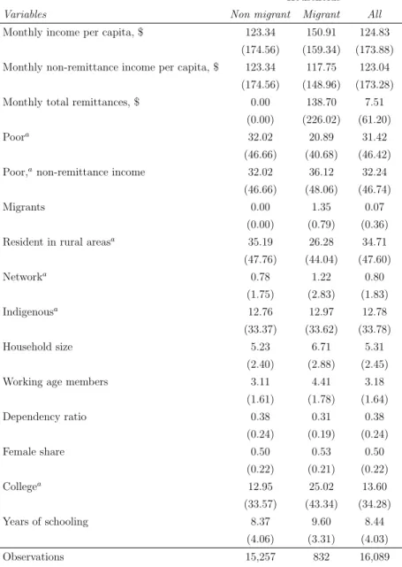
Our final sample includes 16,089 households, with 832 households with at least one mi-gration episode between 1998 and 2005. Table 1 presents the relevant descriptive statistics.
Migrant households have on average 1.35 migrants abroad, with 63.4 and 23.1 percent of them having a migrant in Spain and in the US respectively.
The data reveal that 29.2 percent of the migrant households did not receive remittances in the 12 months before the survey. We defined the subsample of migrant households as including all households that sent at least one migrant abroad between 1998 and 2005, and this implies that some migration episodes actually occurred close to the time of the survey. If we exclude the households who sent their first member abroad in the two years before the survey, the share of non recipient still stands at 26.0 percent.
The incidence of income poverty, defined on the basis of the poverty line set by the INEC,15 stands at 20.9 percent for migrant households; this figure is substantially below
the 36.1 percent that we obtain when defining poverty on the basis of non-remittance in-come only.16 Still, remittances do not represent a revenue that adds up to other exogenous income sources, and they at least partly compensate for the foregone domestic earnings of the migrants,17 and the labor supply decisions of stayers can be endogenous with
re-spect to migration (Chami et al., 2005; Amuedo-Dorantes and Pozo, 2006; Cox-Edwards and Rodr´ıguez-Oreggia, 2009; Binzel and Assaad, 2011). This suggests regarding the incidence of poverty among non migrant households to get a first sense of the impact of migration on poverty. This, as reported in Table 1, stands at 32.2 percent; this implies that the share of poor households is 35.1 percent lower among migrant than among non migrant house-holds. The descriptive statistics reveal that the two groups of households differ with respect to relevant observable characteristics that are likely to be associated both on their poverty status and on the probability to have a migrant. Specifically, a smaller share of the house-holds with at least one member who migrated between 1998 and 2005 reside in rural areas, they have a larger household size and a smaller dependency ratio, and their members are better educated. Migrant households have working age members with 9.6 years of school-ing, while the corresponding figure for non migrant households stands at 8.4 years, in line with the econometric evidence on the determinants of individual self-selection into migration provided by Bertoli (2010) and Bertoli et al. (2011, 2013). Unsurprisingly, the households who recently sent one of their members out of Ecuador have also a better connection with migration networks, proxied by the share of households in each county with a migrant to the US before 1998.
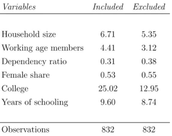
house-holds can be defined either on the basis of all household members, as we did in Table 1, or on the basis of resident members alone. Table 2 reveals that the exclusion of the data on migrant members blurs most of the differences in observables between the two groups of households; beyond the mechanical impact on household size and on the number of working age members, Table 2 shows that migrants are positively selected on education within the household, as the average number of years of schooling falls from 9.6 to 8.7 when we ex-clude migrant members, and the share of households with at least one college graduate falls from 25.02 to 12.95 percent, with the latter figure coinciding with the one for non-migrant households reported in Table 1. This reinforces the empirical relevance of the need to have information on the individual characteristics of migrants, and it gives us a picture of Ecuado-rian migrants that differs from the one assumed by Acosta et al. (2008). This, in turn, has relevant implications for the econometric analysis, as the number and level of education of the migrants clearly exerts an influence upon the poverty status of migrant households in the counterfactual scenario with no migration.
5
Estimates
5.1
Migration and poverty
The treatment z is represented by having at least one household member who left Ecuador between 1998 and 2005, and the outcome y is represented by the poverty status of the household, defined on the basis of the national poverty line.18 We retain the following household characteristics in the vector x of covariates that is used to estimate the propensity score f (x): the number of working age members, the dependency ratio, the share of female working age members, the average years of schooling, a dummy indicating if a household member completed tertiary education, a dummy signaling indigenous self-identification, the county-level size of migration networks,19 a dummy for residence in rural areas.20
The choice of the elements of x, which is constrained by the reasons exposed in Section 3.1.1, is driven by the evidence that emerges from the economic literature. Specifically, the inclusion of variables related to the level of education of the household is motivated by the evidence of large returns to schooling on the Ecuadorian labor market (Bertoli et al., 2011) and of the positive selection on education of recent migrants (Bertoli, 2010). The number and the gender composition of working age members can influence both the probability to send
one its members abroad (Acosta et al., 2007), and it can also be directly related to household income per capita, as the labor productivity in family-run activities is not constant–and labor supply decisions of the household members are mutually interdependent, and Ecuador is characterized by a large gender gap in wages (see, for instance, Bertoli et al., 2013). Geographical factors can shape both the opportunity to migrate and the local incidence of poverty, which is highest in rural areas (Hentschel et al., 2000). Similarly, indigenous households could be, for linguistic and cultural reasons, less likely to migrate, and are also exposed to a higher incidence of poverty (Parandekar et al., 2002).21
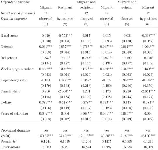
The overall goodness of fit, measured by the pseudo-R2, of the logit model stands at
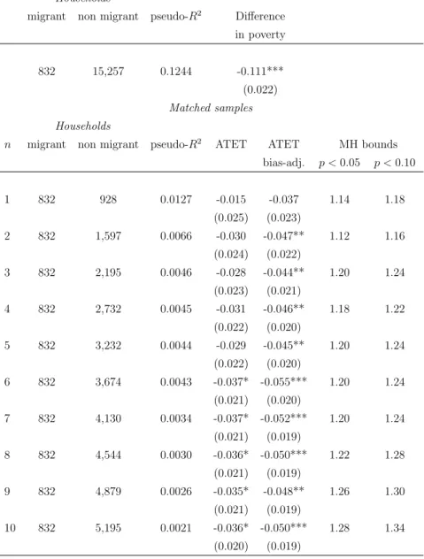
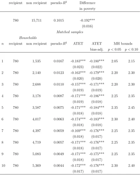
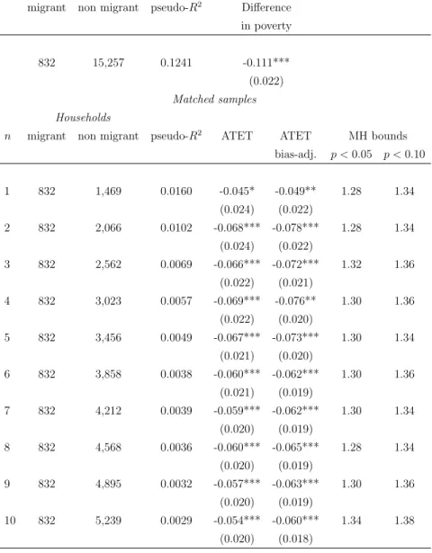
0.124, and specification (1) in Table 3 reports the coefficients that are used to generate the propensity score.22 The estimated propensity score bf (x) is then used to define the subsample of non-migrant households that form the control group, and to estimate the ATET. Table 4 reports the results obtained with nearest neighbor matching, with a number of matches n = 1, ..., 10. The estimation of bf (x) on the subsample of matched households only is characterized by a pseudo-R2 that is 89.8 to 98.3 percent lower than on the whole sample.
The reduction in the pseudo-R2 is increasing in the number of matches n, and it already
stands at 96.3 percent when n = 3, and this is reassuring with respect to the ability of bf (x) to act as a balancing score.
Table 4 reports the estimated ATET: for n ≥ 3, migration induces a decline in the incidence of income poverty between 2.8 and 3.7 percentage points, a figure that stands substantially below the 11.1 percentage points difference reported in Table 1. This suggests that differences in observables, which are controlled for through the matching procedure, account for a large part of the lower incidence of poverty among the households who sent at least one of their member abroad after 1998. Furthermore, the null hypothesis that the ATET is equal to zero can be marginally rejected only for n ≥ 6.
The estimated ATET increases by 1.3-1.6 percentage points for n ≥ 3 when we adopt the regression-based approach proposed by Abadie et al. (2004): the estimates for the bias-adjusted ATET range between -4.4 and -5.5 percentage points, and the null hypothesis that the true effect is zero can always be rejected at least at the 5 percent confidence level. The upper bound of this range implies that migration induced a reduction in the incidence of poverty by 20.8 percent among migrant households. These estimates suggest that differences in observable characteristics can explain no less than half of the observed difference in the
incidence of poverty between migrant and non-migrant households.23
What about possible differences in unobservable characteristics? Table 4 reports the results from the Mantel and Haenszel (1959) test statistic; specifically, it reports the highest values of eγthat still allow to reject at the 5 or 10 percent confidence level the null hypothesis
that the effect of the treatment is zero, with the estimated effect on poverty actually reflecting only a positive selection on unobservables. For n ≥ 3, the estimated ATET is still negative and significant at the 5 percent confidence level for values of eγ ranging between 1.15 and
1.25. This, in turn, implies that an unobserved variable that drives a wedge of 30 percent in the probability to select into migration for otherwise observationally identical households would suffice to fully account for the estimated effect of migration on poverty.
While the test proposed by Becker and Caliendo (2007) is silent about the existence of such a variable, as the conditional independence assumption in (3) is untestable, it suggests that the estimated effect of migration on poverty in Ecuador might reflect even a moderate extent of positive selection on unobservables. The exclusion from the vector x of covariates of any measure of household assets, which is due to the endogeneity of the asset holdings observed at the time of the survey (Bertoli, 2010) and to the absence of retrospective in-formation, implies that concerns about a possible non-random selection on unobservables cannot be readily dismissed. This, in turn, suggests that the ability of the recent wave of migration to reduce the incidence of income poverty in Ecuador might have been limited.
5.2
Remittances and poverty
The survey also allows us to define the treatment as the receipt of remittances. As discussed in Section 4, all households in the sample are asked whether they received remittances from abroad in the month before the survey, as in Acosta et al. (2006, 2008), irrespective of whether they report to have a migrant member.24 We can then define the income of
recipient households as the sum of incomes from all sources, including remittances, reported for November 2005.
No information is provided on the characteristics of the sender of remittances; we in-troduce the same hypotheses as Rodriguez (1998) and Acosta et al. (2008), namely that remittances are sent by one male adult, with the same level of education as non-migrant adults. The incidence of poverty among recipient households stands at 12.8 percent, signif-icantly below the 20.9 percent that characterizes migrant households and 19.2 percentage
points below the corresponding figure for non recipient households.
Specification (2) in Table 3 reports the estimated propensity score bf (x), and Table 5 reports the estimated ATET. With respect to bf (x), we can observe the change in the esti-mated coefficients for the two variables that describe the level of education of the households: the dummy for college education is negative and highly statistically significant, while the average number of years of schooling is no longer significant.25 These changes can be related to the fact that the hypotheses that we introduced about the migrants are at odds with the observed positive selection on education within the household, evidenced by Table 2. Clearly, these changes in bf (x) have an impact on the composition of the control group, and on the estimated ATET.
This becomes apparent from Table 5, where the receipt of remittances is estimated to reduce the share of poor households among recipients between 17.1 and 18.6 percentage points with the bias-adjusted specification of the ATET. These figures correspond to a 57.2-59.2 percent fall in the incidence of poverty,26 well above the 20.8 percent decline that
represented the highest estimated effect obtained when migration represents the treatment variable of interest.
The Mantel and Haenszel (1959) bounds reveal that an unobserved factor that could dou-ble the relative probability of selection into treatment for observationally identical households would not suffice to explain the estimated effect of remittances on poverty. Hence, Table 5 suggests that remittances have a large and highly significant effect on poverty, which is seemingly more robust than the effects reported in Table 4 to a possible non-random selec-tion on unobservables. Nevertheless, the larger values of the Mantel and Haenszel (1959) bounds are due to the reliance on a shorter recall period for remittances, as discussed below in Section 5.3.2, and the likelihood of a positive selection on unobservables substantially increases because of the introduction of hypotheses on the characteristics of the migrants.
5.3
Exploring the difference in the estimates
What can explain the contrast between these estimates, which could provide support to an optimistic view on the poverty-reduction potential of the recent wave of Ecuadorian migration, and the significantly lower effect that we obtained when focusing on migrant households? There are three main factors that can account for this difference,27 namely (i )
recall periods, and (iii ) the introduction of hypotheses on the unreported characteristics of the migrants.
5.3.1 Non-recipient migrant households
As discussed in Section 4, nearly 30 percent of migrant households do not report to have received any transfer from their migrants in the 12 months before the survey. When the treatment is defined as the receipt of remittances, non recipient migrant households are excluded from the group of treated households and this can, in turn, magnify the size of the estimated ATET. We follow two different approaches, which reduce the share of non recipient in the treated group, to gauge the relevance of the difference in the definition of the treatment in accounting for the differences in the ATET reported in Tables 4 and 5.
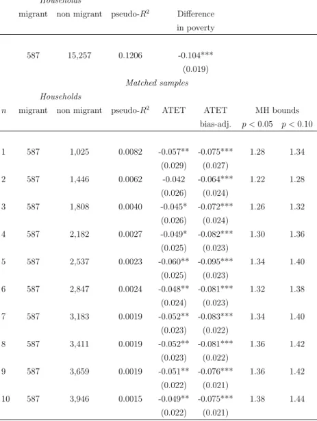
First, we re-define the treatment z as having at least a member who migrated between 1998 and 2005 and receiving remittances over the longer 12-month recall period, and this reduces the number of treated households to 587.28 The estimation of the propensity score is based on the reported individual characteristics of the migrants, as signaled in the third data column in Table 3. The estimated coefficients for the covariates are closer to those obtained in our benchmark specification, with education increasing the probability of exposure to the treatment. Table 6 reports the ATET: migration and the receipt of remittances reduce the incidence of poverty among treated households between 6.4 and 9.5 percentage points, which correspond to a decline in the poverty headcount ratio between 23.4 and 31.3 percent. The estimated effects are more robust to departures from the hypothesis of selection on observables than those in our preferred specification in Table 4.
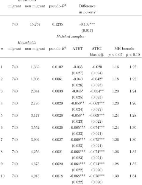
Second, we defined z as having at least one migrant member who migrated between 1998 and 2003, and we drop from the sample the households with their first migration episode in the two years before the survey where the share of non recipient stands at 54.4 percent.29 The fourth data column in Table 3 reports the results of the estimation of bf (x) on this restricted sample, and Table 7 presents the ensuing estimates of the ATET. The bias-adjusted estimated ATET ranges between -5.4 and -7.8 percentage points when n ≥ 3, suggesting that the migration episodes that occurred between 1998 and 2003 reduce the incidence of poverty among migrant households between 20.3 and 26.9 percent, an effect that is larger than in our benchmark specification. This larger effect is consistent with the expectation that, at least initially, the time elapsed since migration increases the likelihood
that the migrant sends remittances back home.
The non-negligible share of migrant households that do not receive remittances over the 12-month recall period thus contributes to explain the different reduction in the incidence of poverty that we find when we define migration or the receipt of remittances as the treatment of interest, but it falls short of accounting for the whole difference.
5.3.2 Different recall periods for remittances
When we focus on migrant households, the ENEMDU 2005 provides information on the remittances received over a period of 12 months, while the focus on recipient households forces us to rely on the amount of remittances reported just for the month before the survey. The shorter recall period can, as discussed in Section 4, induce an over estimation of the income from remittances for recipient households, whenever transfers do not occur on a regular monthly basis.
The average amount of remittances received in November 2005 by recipient households stands at $261.34, significantly above the average monthly amount of remittances received by migrant households over the previous 12 months. Migrant recipient households receive a monthly average amount of remittances equal to $195.80. This implies that the average amount of remittances measured over the shorter recall period exceeds by 33.5 percent the average monthly amount measured over the recall period of one year.
The over estimation in total household income for recipient households induces an un-der estimation in the observed incidence of poverty among recipient households, which Sec-tion 5.2 signaled to stand at 12.8 percent, well below the corresponding figure for migrant households. This, in turn, has a direct implication with respect to the estimated ATET, which depends, as evidenced in (5), linearly on the observed poverty status yi1 of treated
households. Any underestimation of the incidence of poverty among recipient households leads, one to one, to an overestimation of the ATET, and it also increases the Mantel and Haenszel (1959) bounds, whose value is a monotonically increasing function of the share of non-poor treated households (Becker and Caliendo, 2007).
Furthermore, the probability of receiving remittances in the month before the survey is clearly increasing with the frequency with which households receive transfers from their migrants; hence, a shorter recall period for remittances leads to the inclusion in the group of treated of the households that receive a larger number of transfers per year. If the number
of transfers is positively correlated with their aggregate amount, then the group of treated is likely to under-represent the recipient households that receive lower amount of remittances, and this can also induce an upward bias in the estimated effect on poverty.
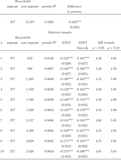
The empirical relevance of these arguments can be assessed if we define the treatment as having at least one migrant member between 1998 and 2005 and having received remittances over the one-month recall period. Such a definition reduces the size of the group of treated to 377 households, with an incidence of poverty that stands at 7.8 percent. This figure is 13.8 percentage points below the one recorded for recipient households when remittances are reported over the 12-month recall period, consistently with the underestimation of the incidence of poverty among recipient households that is induced by the reliance on a shorter recall period to measure a sporadic transfer.
The fifth data column in Table 3 reports the results of the estimation of bf (x) under this definition of the treatment, and Table 8 presents the corresponding ATET. The bias-adjusted ATET reveals a reduction in the incidence of poverty between 16.0 and 19.6 percentage points, an effect that is significantly larger than the 6.4-9.5 percentage points reduction estimated when remittances are measured over the longer 12-month recall period (see Table 6). Furthermore, the estimated effect on poverty appears to be extremely robust to possible departures from the identifying assumption, as an unobservable factor that influences the probability of selection into treatment by a factor of four would not suffice to bring the ATET to zero.
These results entail that the length of the recall period over which remittances are recorded plays a key role in the explanation of the divergence in the results between our preferred approach, which focuses on migration, and the one that defines the receipt of remittances as the treatment of interest.
5.3.3 The hypotheses on the characteristics of the migrants
Household-level data on the receipt of remittances is rarely matched by information on the individual characteristics of the migrant who transfers resources to recipient households. As discussed in Section 3.1.1, the lack this information poses a threat to identification, because some relevant household characteristics become endogenous to migration, and this threat can be mitigated, but not fully addressed, by the introduction of assumptions on the (unknown) characteristics of the migrants.
The availability of individual information on absent members for migrant households gives us the opportunity of assessing the accuracy of the hypotheses. Table 1 evidences that migrant households have on average 1.35 migrant members and Table 1 signals that recent migration flows are gender-balanced, while our estimates in Section 5.2 have been based on the assumption that each recipient household only had one male migrant. Furthermore, and possibly more importantly, Table 2 also reveals that migrants are positively selected on education within each household, and this contrasts with the assumption that migrants have the same level of education as non-migrant members that we retained from Acosta et al. (2008).
How does the discrepancy between the observed characteristics of the migrants and the hypotheses that we adopted influence our estimates? To provide an answer to this question, we re-estimated the effect of migration on poverty disregarding the reported data on migrants and introducing the same assumptions as in Acosta et al. (2008). The results are reported in the sixth data column of Table 3 and in Table 9. The estimated coefficients for the education variables are in line with those reported in specification (2), as households with college education have a lower estimated propensity bf (x) to be exposed to the treatment. The bias-adjusted estimation of the ATET reported in Table 9 reveal that migration reduces the incidence of poverty among migrant households between 4.9 and 7.8 percentage points, with the larger effect corresponding to a 27.2 percent reduction in the poverty headcount ratio. This is in line with the prediction that a systematic error in the measurement of some elements of x for threated households determines a bias in the estimated effect on poverty (Lechner, 2008).
We have provided evidence that points (i )-(iii ) above contribute to explain the difference in the results obtained when focusing on migrant or on recipient households, with the length of the recall period for remittances being the single most relevant factor. The analytical choice of relying on the receipt of remittances to define the treatment of interest, which is often data-driven, produces estimates that are not, in our case, informative about the direct influence of international migration on poverty.
6
Concluding remarks
Our analysis reveals that the wave of migration that was triggered by the late-1990s economic crisis in Ecuador has induced a decline in the incidence of poverty among migrant households, that is estimated between 17.4 and 20.8 percent and which might also reflect a positive selection on unobservables. The availability of data on migrants and the measurement of remittances over a 12-month recall period proved to be critical in our analysis. The standard, and less data-demanding, choice to focus on the receipt of remittances as the treatment of interest would have produced a significantly larger estimated effect on poverty. The substantial share of non recipient migrant households only partly explains the difference between the two estimates, which is also driven by the shorter recall period for remittances and by the introduction of hypotheses on the characteristics of migrant members. The high migration costs that most would-be migrants faced at the end of the 1990s (Bertoli et al., 2013) probably contributed to limit the direct poverty-reduction potential of the Ecuadorian exodus, as they hindered poor households from sending one of their members abroad.
References
Abadie, A., D. Drukker, J. L. Herr, and G. W. Imbens (2004): “Implementing matching estimators for average treatment effects in Stata,” Stata Journal, 4(3), 290–311.
Abadie, A., and G. W. Imbens (2008): “On the Failure of the Bootstrap for Matching Estimators,” Econometrica, 76(6), 1537–1557.
Acosta, P. (2011): “School Attendance, Child Labour, and Remittances from International Migration in El Salvador,” Journal of Development Studies, 47(6), 913–936.
Acosta, P., C. Calder´on, P. Fajnzylber, and H. L´opez (2006): “Remittances and Development in Latin America,” World Economy, 29(7), 957–987.
(2008): “What is the Impact of International Remittances on Poverty and Inequality in Latin America?,” World Development, 36(1), 89–114.
Acosta, P., P. Fajnzylber, and H. L´opez (2007): “The Impact of Remittances on Poverty and Human Capital: Evidence from Latin American Household Surveys,” in In-ternational Migration, Economic Development and Policy, ed. by C. ¨Ozden,andM. Schiff, pp. 59–98. Washington: The World Bank.
Adams, R. H. (1989): “Worker Remittances and Inequality in Rural Egypt,” Economic Development and Cultural Change, 38(1), 45–71.
(2011): “Evaluating the Economic Impact of International Remittances On Devel-oping Countries Using Household Surveys: A Literature Review,” Journal of Development Studies, 47(6), 809–828.
Adams, R. H., and A. Cuecuecha (2013): “The Impact of Remittances on Investment and Poverty in Ghana,” World Development, 50, 24–40.
Agarwal, R., and A. W. Horowitz (2002): “Are International Remittances Altruism or Insurance? Evidence from Guyana Using Multiple-Migrant Households,” World Devel-opment, 30(11), 2033–2044.
Amuedo-Dorantes, C., and S. Pozo (2006): “Migration, Remittances, and Male and Female Employment Patterns,” American Economic Review, 96(2), 222–226.
Barham, B., and S. Boucher (1998): “Migration, remittances, and inequality: estimat-ing the net effects of migration on income distribution,” Journal of Development Eco-nomics, 55(2), 307–331.
Becker, S.,and M. Caliendo (2007): “Sensitivity analysis for average treatment effects,” Stata Journal, 7(1), 71–83.
Beckerman, P., and H. Cort´es-Douglas (2002): “Ecuador under Dollarization: Op-portunities and Risks,” in Crisis and Dollarization in Ecuador, ed. by P. Beckerman, and
A. Solimano, pp. 81–126. Washington: The World Bank.
Beine, M., F. Docquier, and M. Schiff (2013): “International migration, transfer of norms and home country fertility,” Canadian Journal of Economics, 46(4), 1406–1430.
Bertoli, S. (2010): “Networks, sorting and self-selection of Ecuadorian migrants,” Annales d’ ´Economie et de Statistique, 97/98, 261–288.
Bertoli, S., J. Fern´andez-Huertas Moraga, and F. Ortega (2011): “Immigration Policies and the Ecuadorian Exodus,” World Bank Economic Review, 25(1), 57–76.
(2013): “Crossing the Border: Self-Selection, Earnings and Individual Migration Decisions,” Journal of Development Economics, 101(1), 75–91.
Bertoli, S., and F. Marchetta (2013): “Bringing It All Back Home – Return migration and the transfer of fertility norms,” World Development, forthcoming.
Binzel, C., and R. Assaad (2011): “Egyptian men working abroad: Labour supply responses by the women left behind,” Labour Economics, 18(S1), S98–S114.
Calero, C., A. Bedi, and R. Sparrow (2009): “Remittances, Liquidity Constraints and Human Capital Investments in Ecuador,” World Development, 37(6), 1143–1154.
Caliendo, M., and S. Kopeinig (2008): “Some Practical Guidance for the Implementa-tion of Propensity Score Matching,” Journal of Economic Surveys, 22(1), 31–72.
Chami, R., C. Fullenkamp, and S. Jahjah (2005): “Are Immigrant Remittance Flows a Source of Capital for Development?,” IMF Staff Papers, 52(1), 55–81.
Chiquiar, D., and G. H. Hanson (2005): “International Migration, Self-Selection, and the Distribution of Wages: Evidence from Mexico and the United States,” Journal of Political Economy, 113(2), 239–281.
Cox-Edwards, A., and E. Rodr´ıguez-Oreggia (2009): “Remittances and Labor Force Participation in Mexico: An Analysis Using Propensity Score Matching,” World Develop-ment, 37(5), 1004–1014.
de la Fuente, A. (2010): “Remittances and Vulnerability to Poverty in Rural Mexico,” World Development, 38(6), 828–839.
Dehejia, R. (2005): “Practical propensity score matching: a reply to Smith and Todd,” Journal of Econometrics, 125(12), 355 – 364.
Dehejia, R. H., and S. Wahba (2002): “Propensity Score-Matching Methods For Non-experimental Causal Studies,” The Review of Economics and Statistics, 84(1), 151–161.
Docquier, F., and H. Rapoport (2012): “Globalization, brain drain and development,” Journal of Economic Literature, 50(3), 681–730.
Fern´andez-Huertas Moraga, J. (2011): “New Evidence on Emigrant Selection,” The Review of Economics and Statistics, 93(1), 72–96.
(2013): “Understanding different migrant selection patterns in rural and urban Mexico,” Journal of Development Economics, 103, 182–201.
Fr¨olich, M. (2007): “Propensity score matching without conditional independence as-sumptionwith an application to the gender wage gap in the United Kingdom,” Economet-rics Journal, 10(2), 359–407.
Gray, C. L. (2009): “Environment, Land, and Rural Out-migration in the Southern Ecuadorian Andes,” World Development, 37(2), 457–468.
Gustafsson, B., and N. Makonnen (1993): “Poverty Remittances in Lesotho,” Journal of African Economies, 2(1), 49–73.
Hentschel, J., J. O. Lanjouw, P. Lanjouw, and J. Poggi (2000): “Combining Census and Survey Data to Trace the Spatial Dimensions of Poverty: A Case Study of Ecuador,” World Bank Economic Review, 14(1), 147–165.
Ho, D. E., K. Imai, G. King, and E. A. Stuart (2007): “Matching as Nonparametric Preprocessing for Reducing Model Dependence in Parametric Causal Inference,” Political Analysis, 15(3), 199–236.
Ichino, A., F. Mealli, and T. Nannicini (2008): “From temporary help jobs to perma-nent employment: what can we learn from matching estimators and their sensitivity?,” Journal of Applied Econometrics, 23(3), 305–327.
Imai, K., G. King,and E. A. Stuart (2008): “Misunderstandings between experimental-ists and observationalexperimental-ists about causal inference,” Journal of the Royal Statistical Society: Series A (Statistics in Society), 171(2), 481–502.
J´acome, L. I. (2004): “The Late 1990s Financial Crisis in Ecuador: Institutional Weak-nesses, Fiscal Rigidities, and Financial Dollarization at Work,” IMF Working Paper No. 04/12.
Jimenez-Soto, E. V., and R. P. C. Brown (2012): “Assessing the Poverty Impacts of Migrants’ Remittances Using Propensity Score Matching: The Case of Tonga,” Economic Record, 88(282), 425–439.
Jokisch, B., and J. Pribilsky (2002): “The Panic to Leave: Economic Crisis and the New Emigration from Ecuador,” International Migration, 40(4), 75–102.
Lechner, M. (2008): “A note on endogenous control variables in causal studies,” Statistics and Probability Letters, 78(2), 190–195.
Lee, W.-S. (2013): “Propensity score matching and variations on the balancing test,” Empirical Economics, 44, 47–80.
Leliveld, A. (1997): “The effects of restrictive South African migrant labor policy on the survival of rural households in Southern Africa: A sase study from rural Swaziland,” World Development, 25(11), 1839–1849.
Lokshin, M., M. Bontch-Osmolovski, and E. Glinskaya (2010): “Work-Related Migration and Poverty Reduction in Nepal,” Review of Development Economics, 14(2), 323–332.
Mantel, N., and W. Haenszel (1959): “Statistical aspects of the analysis of data from retrospective studies,” Journal of the National Cancer Institute, 22, 719–748.
Marchetta, F. (2012): “Migration and the Survival of Entrepreneurial Activities in Egypt,” World Development, 40(10), 1999–2013.
McKenzie, D. J., and H. Rapoport (2010): “Self-selection patterns in Mexico-U.S. migration: The role of migration networks,” The Review of Economics and Statistics, 92(4), 811–821.
McKenzie, D. J., S. Stillman, and J. Gibson (2010): “How Important is Selection? Experimental VS. Non-Experimental Measures of the Income Gains from Migration,” Journal of the European Economic Association, 8(4), 913–945.
Mishra, P. (2007): “Emigration and wages in source countries: Evidence from Mexico,” Journal of Development Economics, 82(1), 180–199.
Mountford, A., and H. Rapoport (2011): “The brain drain and the world distribution of income,” Journal of Development Economics, 95(1), 4–17.
Nannicini, T. (2007): “Simulation-based sensitivity analysis for matching estimators,” Stata Journal, 7(3), 334–350.
Parandekar, S., R. Vos, and D. Winkler (2002): “Ecuador: Crisis, Poverty and Social Protection,” in Crisis and Dollarization in Ecuador, ed. by P. Beckerman, and
A. Solimano, pp. 127–176. World Bank.
Peikes, D. N., L. Moreno, and S. M. Orzol (2008): “Propensity Score Matching: A Note of Caution for Evaluators of Social Programs,” The American Statistician, 62(3), 222–231.
Rodriguez, E. (1998): “International Migration and Income Distribution in the Philip-pines,” Economic Development and Cultural Change, 46(2), 329–350.
Rosenbaum, P. R. (2002): Observational Studies. New York: Springer.
Rosenbaum, P. R., and D. B. Rubin (1983): “The central role of the propensity score in observational studies for causal effects,” Biometrika, 70(1), 41–55.
Schiff, M. (2008): “On the underestimation of migration’s income and poverty impact,” Review of Economics of the Household, 6(3), 267–284.
Sianesi, B. (2004): “An Evaluation of the Swedish System of Active Labor Market Pro-grams in the 1990s,” The Review of Economics and Statistics, 86(1), 133–155.
Smith, J. A., and P. E. Todd (2005a): “Does matching overcome LaLonde’s critique of nonexperimental estimators?,” Journal of Econometrics, 125(12), 305 – 353.
(2005b): “Rejoinder,” Journal of Econometrics, 125(12), 365 – 375.
Stark, O., and D. Bloom (1985): “The New Economics of Labor Migration,” American Economic Review, 75(2), 173–178.
Wahba, J., and Y. Zenou (2012): “Out of Sight, Out of Mind: Migration, Entrepreneur-ship and Social Capital,” Regional Science and Urban Economics, 42(5), 890–903.
Woodruff, C., and R. Zenteno (2007): “Migration networks and microenterprises in Mexico,” Journal of Development Economics, 82(2), 509–528.
World Bank (2012): World Development Indicators. Washington: the World Bank.
Yang, D. (2008): “International Migration, Remittances and Household Investment: Evi-dence from Philippine Migrants Exchange Rate Shocks,” The Economic Journal, 118(528), 591–630.
Yang, D., and C. Martinez (2007): “Remittances and poverty in migrants home areas: evidence from the Philippines,” in International Migration, Economic Development and Policy, ed. by C. ¨Ozden,and M. Schiff, pp. 81–122. Washington: The World Bank.
Zanutto, E. L. (2006): “A Comparison of Propensity Score and Linear Regression Analysis of Complex Survey Data,” Journal of Data Science, 4(1), 67–91.
Notes
1The expression “migrant household” is used throughout this paper to denote a household that resides at origin and that has sent at least one of its members abroad.
2See Adams (2011) for a recent survey of the analytical challenges posed by the use of household-level data to analyse the effects of remittances on migrant-sending countries.
3The share of households with at least one migrant that do not receive remittances stands, for instance, at 41 percent for Nicaragua in Barham and Boucher (1998) and at 37 percent for Guyana in Agarwal and Horowitz (2002).
4Notice that this analysis is not meant to isolate the effect of remittances on poverty, opposed to a distinct effect of migration.
5Caliendo and Kopeinig (2008) provide an excellent survey of the analytical choices involved in the implementation of this estimation method.
6The availability of data on migrants allows us to fully account for the migration-induced variation in household-size, thus avoiding the risk, which is pointed out by Schiff (2008), of underestimating the effect of migration on poverty.
7An alternative approach to reduce the concerns about endogeneity is to introduce explicit assumptions about the migrant members, when these are unobserved; for instance, Acosta et al. (2008) follow Rodriguez (1998), assuming that “remittances are sent by an adult male family member, who has the average years of education of other adults in the household” (p. 99).
8All the results presented in Section 5 are robust to the exclusion from the sample of the households residing in these two provinces.
9The limited time elapsed since the treatment also mitigates the concern about the direct and opposite effects of migration on the number of dependent members in the household, due to the reduction in the opportunities for sexual intercourse between the migrant and the spouse left behind and to the improved chances of survival of older members due to a migration-induced increase in consumption.
10See, for instance, Acosta et al. (2006, 2008) and Calero et al. (2009) for analyses on Ecuadorian data. 11Specifically, the asset index, which is built by Bertoli (2010) only on the basis of the assets that are “more likely to reflect past savings” (Acosta, 2011, p. 919), is an increasing function of the years passed since migration; this might reflect either the positive effect of remittances or the depletion of household assets to cover the monetary costs of migration, or both.
12This choice is in line with McKenzie et al. (2010), who observe that “among the other non-experimental methods, difference in-differences and propensity score matching with bias-adjustment work best” (p. 942) when estimating the income gains from migration.
13See Caliendo and Kopeinig (2008) for an overview of the alternative approaches to test the sensitivity of the estimates to the existence of confounders.
14The exclusion of recipient households with no migrants is motivated by the idea that a large share of these households could be actually mis-reporting with respect to the existence of a migrant, although this group also certainly includes recipient households belonging to the extended family of the migrants; the