Landlockedness, Infrastructure and Trade:New Estimates for Central Asian Countries

HAL Id: halshs-00556941

https://halshs.archives-ouvertes.fr/halshs-00556941

Preprint submitted on 18 Jan 2011

HAL is a multi-disciplinary open access

archive for the deposit and dissemination of sci-entific research documents, whether they are pub-lished or not. The documents may come from teaching and research institutions in France or abroad, or from public or private research centers.

L’archive ouverte pluridisciplinaire HAL, est destinée au dépôt et à la diffusion de documents scientifiques de niveau recherche, publiés ou non, émanant des établissements d’enseignement et de recherche français ou étrangers, des laboratoires publics ou privés.

Céline Carrere, Christopher Grigoriou

To cite this version:

Céline Carrere, Christopher Grigoriou. Landlockedness, Infrastructure and Trade:New Estimates for Central Asian Countries. 2011. �halshs-00556941�

Document de travail de la série Etudes et Documents E 2008.01

L

L

AANNDDLLOOCCKKEEDDNNEESSSS

,

,

I

I

NNFFRRAASSTTRRUUCCTTUURREEAANNDD

T

T

RRAADDEE

:

:

N

N

EEWW

E

E

SSTTIIMMAATTEESSFFOORR

C

C

EENNTTRRAALL

A

A

SSIIAANN

C

C

OOUUNNTTRRIIEESS Carrère Céline* Grigoriou Christopher** January, 2008 29 p.

* CERDI-CNRS, Université d’Auvergne, FRANCE, Celine.Carrere@u-clermont1.fr

A

ABBSSTTRRAACCTT

This paper assesses the impact of internal infrastructure and landlockedness on Central Asian trade. The impact of landlockedness on Central Asian’s trade costs is split into several components, using a panel gravity equation estimated on a large sample of countries (167 countries over 1992-2004). Our findings highlight that an improvement in the own infrastructure of Central Asian countries from the level of the median Central Asian country to that of other landlocked countries would raise exports (imports) by a modest 2.4% (3.1%). By contrast, an improvement in Central Asian transit-country infrastructure to the level of the other landlocked countries would raise the representative CAC’s exports by a whopping 49%. Other dimensions of landlockedness considered in this study are also great impediments to trade. Either diminishing the extra overland costs or enhancing the ability to negotiate sea access would significantly increase Central Asian trade, ‘’transit monopolies’’ (single transit corridors) reducing trade significantly.

Keywords: Central Asia, Landlockedness, Trade, Transport Infrastructure, Panel data.

1. INTRODUCTION

The Soviet Union’s collapse in the 1990s was expected to lead to a major reorientation of the former bloc’s trade, given that politically-determined trade links under central planning had given rise to substantial over-trading between former Soviet Union states. For instance, Fidrmuc and Fidrmuc (2003) estimated that former Soviet Union countries traded 43 times more between them than predicted by GDP and distance. Conversely, Hamilton and Winters (1992) and Baldwin (1994) calculated that potential trade between former Soviet Union countries and the EU was more than four times the actual volume. However, by the late 1990s, if trade with the Soviet Union had indeed shrunk, reorientation was limited as trade with other regions had failed to take off. By 1998, for instance, trade between Russia and former Soviet Union countries, although reduced, was still 30 times greater than ‘normal’ (Fidrmuc and Fidrmuc 2003). Designing policies to assist the Central Asian Countries (CACs)1 _{to achieve the}

reorientation of their foreign trade and integrate in the global economy requires an understanding of the nature of their handicaps that goes beyond the mechanical effect of landlockedness. What is needed is an understanding of (i) how the effect of landlockedness interacts with that of poor infrastructure in the CACs and in neighboring (transit) countries; and (ii) what practical policy steps can help mitigating the effect of landlockedness on trade.

The literature so far explains hysteresis in former Soviet Union trade by remoteness and landlockedness2 _{(Kaminski, Wang and Winters, 1996; Djankov}

and Freund, 2002; Grafe, Raiser and Sakatsume, 2005), poor access to markets and incomplete reforms (Havrylishin and Al-Atrash, 1998), weak institutions (Babetskaia-Kukharchuk and Maurel, 2004), poor product quality (e.g. Bevan et al., 2001), and hysteresis in consumption, production and business networks (Djankov and Freund, 2002).

Beyond Central Asia, a voluminous gravity-based literature has also provided estimates, often incidental, of the impact of landlockedness on trade. Typically, these studies included a dummy variable equal to one for landlocked countries. For instance, Carrère (2006) found that, on the basis of a panel gravity model, ceteris paribus a landlocked country traded about 28% less than a coastal one. Estimates of similar magnitudes were found in other studies. Clearly, these estimates could explain only a small part of the CACs’ under-trading with the rest of the world. Indeed, few of those papers focused explicitly on the impact of landlockedness on trade. One notable exception was Raballand (2003) who analyzed the effect of landlockedness on trade in the case of Central Asian countries. Using a restricted sample of 46 CIS countries, 18 of which landlocked, over a period of 5 years (1995-1999), he found landlockedness to reduce trade by more than 80%. This very large impact, substantially out of step with usual estimates, was at least partly due to the fact that his landlockedness variable was equal to one only for bilateral trade between two landlocked countries, while the

1 _{Throughout this paper, by Central Asian Republics, we mean Kazakhstan, the Kyrgyz Republic,}

Tajikistan, Turkmenistan, and Uzbekistan.

2 _{Only Kazakhstan and Turkmenistan have access to the Caspian Sea, itself a landlocked sea}

bordered only by Russia, Azerbaijan and Iran, while Uzbekistan is twice landlocked, i.e. surrounded by countries that are themselves landlocked.

landlockedness variable in other studies usually marks the bilateral trade of landlocked countries with all their partners, landlocked or not.

Dummy variables in a gravity equation are black boxes that do not tell us much about how landlockedness affects trade. A limited number of studies have shed light on the channels through which its impact is felt. In his study of Central Asian trade, Raballand (2003) introduced two components of landlockedness ---shortest distance to a major port facility and number of borders crossed in transit, and found them to have significant effects. Using CIF/FOB data from the IMF for 97 developing countries, 17 of which landlocked, Radelet and Sachs (1999) estimated that transport and insurance costs were twice as high for landlocked countries as for coastal countries. They concluded that “geographic isolation and higher shipping costs may make it much more difficult if not impossible for relatively isolated developing countries to succeed in promoting manufactured exports”. Limao and Venables (2001) found a large effect of infrastructure development on trade costs, in particular for landlocked countries, on the basis of a cross section of countries with controls for the level of transit-country infrastructure. The high impact of remoteness and infrastructure on trade costs was also evidenced by Brun et al. (2005). Using IMF estimations of freight payments as a percentage of imports, Stone (2001) found a comparable transport cost burden. The transport costs were lower in transit states than in landlocked countries in 75% of the cases, from the 64 possible comparisons between landlocked countries and transit countries.

In this paper, we revisit the evidence using a large panel of bilateral trade flows between 167 countries over 13 years spanning 1992-2004. Particular attention is given to the econometric specification of the gravity model in order to eliminate sources of biases common in conventional gravity models. In particular, we take advantage of the sample’s panel structure to include country-pair specific effects instead of the usual exporter and importer effects (making the identification of time-invariant country characteristics like landlockedness possible) and treat carefully the potential endogeneity of some of the explanatory variables. Using this proper specification, we assess the impact of domestic infrastructure and landlockedness on Central Asian trade and provide a decomposition of landlockness’ impact on transport costs into several components, such as overland distance to port or transit-country infrastructure.

Our empirical results show that an improvement in the own infrastructure of Central Asian countries from the level of the median Central Asian country to that of other landlocked countries would raise exports (imports) by a modest 2.4% (3.1%).3 _{In the same way, an improvement in Central Asian infrastructure}

network to the level of the median coastal country would raise exports (imports) by 14.5% (19.6%). Thus, the impact of domestic infrastructure appears limited.4

By contrast, an improvement in Central Asian transit-country infrastructure to the level of the other landlocked countries would raise the representative CAC’s exports by a whopping 49%. Other dimensions of landlockedness considered in this study are also great impediments to the trade of Central Asian countries.

3 _{Maintaining all other variables at the level of the representative Central Asian country (median}

value).

4 _{And not specific to landlocked countries as the associated coefficient is the same for all countries}

Hence, diminishing the extra overland costs (proxied by the distance to the nearest port) or enhancing the ability of a landlocked country to negotiate sea access compared to others landlocked countries would significantly increase Central Asian trade, ‘’transit monopolies’’ (single transit corridors) reducing trade significantly.

The paper is organized as follows. Section 2 presents some stylized facts on infrastructure and geographical disadvantages of Central Asia. Section 3 develops the assessment method of the impact of infrastructure and landlockedness on the Central Asian trade. Section 4 details the results. Section 5 provides some concluding remarks and suggests some induced policy recommendations.

2. STYLIZED FACTS ON INFRASTRUCTURE AND GEOGRAPHICAL

DISADVANTAGES OF CENTRAL ASIA

High transport costs are certainly one of the main impediments to the reorientation of Central Asian trade. The distance of Central Asian countries from the main economic markets is of course only part of the story5_{. The density and}

quality of internal infrastructure are also determining factors of Central Asian trade costs, though perhaps more important in terms of trade policy. Limao and Venables (2001) emphasized that distance explains only 10% of changes in transport costs. Poor road infrastructure represents 40% of the transport costs predicted for coastal countries and 60% for landlocked countries. We shall show that this is particularly relevant for Central Asian countries.

However, distance and internal infrastructure alone do not explain why Central Asian countries are at a disadvantage even compared to countries with similar infrastructure endowments or which are similarly remote but which have sea access. Once low incomes, a poor internal infrastructure network, distance and remoteness are controlled for statistically, landlockedness still has a negative and highly significant impact on trade (see Limao and Venables 2001, Raballand 2003 or Carrère 2006). There are many reasons for this. For instance, overland distances are more penalizing than sea distances because of their higher costs per mile. Moreover, landlocked countries are dependent on sovereign transit countries for their trade, a dependency that may only serve to compound existing problems.

We present direct estimates of transport costs for Central Asia in Section 2.1. The internal infrastructure of Central Asian countries is analyzed in Section 2.2., while the specific costs of landlockedness are discussed in Section 2.3.

2.1 Direct estimates of Central Asian transport costs

Direct estimates of transport costs have been gathered from a survey of transport firm managers along various routes linking Europe and Central Asia (see Raballand et al., 2005). They show that the cost of transporting a 40’ container by

5 _{See World Bank (2004) for an illustration of the main route corridors and distances for}

international freight movements to and from the main trade centers of the region. The five Central Asian countries are clearly remote from the main global markets.

road rises by and large linearly with the distance; a slightly higher derivative was recorded for the Central European leg of the journey (between Warsaw and Moscow). However, the cost of transporting a 20’ container by rail rises less than proportionately with the distance after the Moscow leg. Although Raballand et al. do not offer any reasons why this is the case, it is likely that these cost differences reflect the politically motivated subsidization of freight rates in the former CIS.6

The same picture emerges for transport times. Unlike costs, time rises more than proportionately with distance after the Moscow leg, which reflects more difficult conditions for both rail and road cargo. Similar observations have been made for the trade route between the US and Central Asia.7 _{Aside from a change in}

transport costs and time per kilometer, it is worth noting that long distances produce extremely high transport costs (USD 6,000 for a 40’ container from Paris to Tashkent, a prohibitive level for most types of cargo).

2.2 Internal infrastructure: a common component of transport costs across all countries

The relation between infrastructure and trade are supported by both theoretical (e.g. Bougheas, Demetriades and Morgenroth, 1999) and empirical evidence (see Limao and Venables, 2001). Limao and Venables (2001), using a combination of shipping data and CIF/FOB ratios, have shown that a deterioration in the infrastructure from the median to the 25th _{percentile raised transport costs by 12}

percentage points and reduced trade volumes by 28 percent. The issue of inadequate infrastructure is of particular relevance for Central Asia.

Estache and Goicoechea (2005) have shown that Central Asia has low levels of transport and communications’ infrastructure. For instance, railway density is on average 5.4 rail-km per 1,000 sq. km, i.e. one-third of the average railway density of low- and middle-income countries. This is a particular cause for concern given that approximately 90% of total freight transport in Central Asian countries during 2000 was by rail (see Raballand et al. 2005). It is therefore fair to say that low infrastructure levels are likely to affect Central Asian trade, and that the lack of investment in existing infrastructure increases transport costs.

Given the availability on the data regarding roads and rails, we use the indicator from Limao and Venables (2001). It is commonly used since in the literature to assess the infrastructure level in international trade studies, even if it focuses on quantitative aspects of infrastructre rather than on qualitative ones.8

6 _{It should be noted, however, that freight rates on routes between Moscow and Central Asian}

capitals are differentiated in terms of cargo, with low rates applying to primary product shipments (e.g. cotton from Uzbekistan) from Central Asia to Russia. We are grateful to Eskender Trushin from the Tashkent Bureau of the World Bank for pointing this out.

7 _{For instance, Stone (2001) notes that freight rates per mile are twice as high for a container}

shipped to Bishkek (Kyrgyzstan) than for one shipped to Ankara.

8 _{With this indicator, we ignore other important aspects of infrastructure such as maintenance and}

services. See for instance the Asian Bank of Development Bank (2006) that documented a trend of deteriorating material and infrastructure, primarily as the result of inadequate maintenance (notably for railway infrastructure). According to Pomfret (2005), the insufficient funding earmarked for infrastructure maintenance is a phenomenon common to all former Soviet countries, where national networks often take precedence over regional networks. Fot the negative impact resulting from inadequate road maintenance see Cadot, Dutoit and de Melo 2005; Cadot, Dutoit

2.3 Additional costs of landlockedness in Central Asian countries Landlocked countries often lag behind their maritime neighbors in terms of external trade and economic development, even when they have similar distances to main trade partners or similar internal transport infrastructure. The reason is that landlocked countries also have to cope with long overland distances (notably to join ports) and are largely dependent on sovereign transit countries, which they have to cross in order to access international shipping markets (see Faye et al., 2004, Ojala, 2005, or Carcamo-Diaz, 2004 for surveys on the various forms of transit dependency).

Overland distance

Landlockedness affects many countries, but some, such as Switzerland, nonetheless manage to prosper. However, the story is altogether different for Central Asia. Except for Batumi on the Black Sea (which can be reached only after trans-shipment over the Caspian Sea), all ports are more than 3,000 km away from their closest Central Asian border. Many are even farther away, the shortest route to the sea being the Southern one which happens to go through what is probably the most unstable region of the world. Such huge land distances imply problems of a different magnitude than those faced by European landlocked countries like Switzerland and the Czech Republic, which are 500-600 km away from major ports.

In terms of monetary transport costs (one dimension of the problem, although by no means the only one), Limao and Venables (2001) estimated that overland transport costs rise by as much as $1,380 per 1,000 km compared to only $190 for overseas transport.

Finally, freight costs lie roughly in the $1,000-3,000 range for distances between 3,000 and 5,000 km, suggesting average rates of less than $500 per thousand kilometers. Although the shortest route is the Afghan one to Karachi via Quetta, the Bandar Abbas rail route appears the most attractive. Taking this as a basis for our calculations, maintaining the freight rate below 10% of shipment value (a high rate given that it covers only overland transport to the port of destination) implies a cargo worth at least $15,000, a very high value for a 20’ container −and one that would be risky to ship on a hazardous route.

Transit infrastructure

Landlocked countries are completely dependent on their transit neighbors’ infrastructure to transport their goods to the nearest port. There are many causes of weak infrastructure, including lack of resources, poor governance, conflict and natural disasters. Regardless of the cause, weak infrastructure impose direct costs on trade passing through transit countries and thus limit the ability of products and Olarreaga (2005) and especially Raballand et al. (2005) in the case of Kazakhstan. On the “soft” aspects of the transit sector’s business environment, see “logistics friendliness” survey (based on data provided by approximately ten companies involved in international transport and trade in Central Asia, Asian Development Bank (2006)). However, the lack of data does not allow us to take explicitly into accounts these factors.

from landlocked countries to compete in global markets. The relative impact of the weak infrastructure of its neighbors has a particularly negative impact on those landlocked countries which mainly export primary commodities with low value-to-cost ratios rather than high-value products or services. A weak infrastructure of a transit country also limits the return to investment in landlocked countries’ internal infrastructure due to the restrictions it places on market opportunities. The data yielded by CIF/FOB ratios allowed Limão and Venables (2001) to estimate that improving the infrastructure of transit countries, all other things being equal, would reduce the transport cost differential between the median landlocked economy and the median coastal country from 46% to 43%, and thus lead to a 2% increase in trade volume.

Transport infrastructure in the Central Asia sub-region has been heavily influenced by the needs of the former Soviet Union, with road and rail networks designed to facilitate traffic flows towards the European part of Russia, particularly Moscow and Ukraine. Road and rail connections are less well developed both within Central Asia itself, and between Central Asia and its neighbours to the east and south. Connections through China, Iran, Afghanistan and Pakistan are limited and poorly developed. There is one major paved road corridor through the sub-region, running east to west and linking Tashkent to Almaty, with connecting roads to China and Turkmenistan. There is also a single rail corridor to China, passing through the high mountains of the Kazakh-China border. For more details on the major trade corridor for Central Asian Trade, see Ojala (2005).

However, the practicability of transit corridors depends not only on the physical infrastructure of transit countries but also on their political climate and on the quality of their governance, which, in the case of Central Asia’s transit partners, is a particular cause for concern.

Difficult neighbor relations and Limited choice of transit corridors Landlocked countries are heavily dependent on their political relations with transit countries. If there is conflict, whether military or diplomatic, between a landlocked country and its transit neighbors, the latter can easily block borders or set up regulatory impediments to trade. Even where there is no direct conflict, landlocked countries are vulnerable to the political vagaries of their neighbors. According to Faye et al. (2004), “although there is a legal basis for rights of landlocked transit as outlined in Article 125(1) of the United Nations Convention on the Law of the Sea (United Nations, 1982), in practice, this right of access must be agreed upon with the transit neighbour (Article 125(2) and (3)) and is determined by the relationship between the countries.”

As these authors also pointed out, Central Asian Republics have been badly affected by cross-border disputes. After the collapse of the USSR, the former Soviet republics were divided along previous administrative boundaries, which have since been the source of many disputes. As a result, borders are regularly

defended with landmines and physical blockades.9 _{Ongoing tensions have also}

resulted in a general failure of regional cooperation.

Finally, the limited choice of transit corridors does not allow Central Asian countries to negotiate with transit countries. Some new transit agreements are in development, but at the present time a number of transit countries continue to exercise a monopoly. As noted by UNESCAP 2003, this restricted competition in Central Asia in the provision of transit transport services between operators, modes of transport and routes may result in inefficient pricing policies and services.

3. ASSESSING THE IMPACT OF INFRASTRUCTURE AND LANDLOCKEDNESS ON CENTRAL ASIAN TRADE

In this section we will address two important issues. First, to what extent is Central Asian trade affected by the level of internal infrastructure network? Second, how far is it reduced by higher transport costs due to landlockedness? The gravity equation provides a general empirical framework and is especially suited to the examination of these issues. This model allows us to identify the impact on bilateral trade of variables, such as infrastructure and landlockedness, once all other structural determinants of trade, mainly GDP, distance and remoteness, are controlled for. The gravity model is presented in detail below. 3.1. Derivation of the gravity equation with infrastructure and landlockedness

We use the gravity model as a simple and efficient tool to predict the volume of bilateral trade and to assess the burden of landlockedness (see surveys proposed by Evenett and Keller, 1998, Anderson and van Wincoop, 2004, and Feenstra, 2004). We adopt the popular version of the gravity model currently applied when aggregating trade between economies with an assumed specialization in differentiated products. As shown by Deardoff (1998), as well as Anderson and Van Wincoop (2003, 2004), the utility maximization of an identical (over countries) CES utility function yields the following expression for bilateral imports, 1 it jt ijt ijt wt it jt Y Y M Y R R σ

θ

−     = _ _  _  (1)

where M_ijt is the CIF (cost, insurance and freight) value of the aggregate merchandise trade flow imported by country i from exporter j; Y_{i j t( )} is the gross

9 _{Moreover, according to the World Bank (2005), the most serious problem relates to customs and}

the incidence of unofficial payments, which is extraordinarily pernicious in Central Asia. This handicap compounds other customs-related impediments, such as the lack of coordination among border-related agencies, complexity of customs’ procedures, lack of transparency in customs’ codes and regulations, low utilization of information technology in customs’ operations, as well as long transit times. The lack of data does not allow us to take explicitly into accounts these factors.

domestic product of country i (j) in t; Y_wtis the world income in t, θijt is bilateral

transport costs; σ is the elasticity of substitution in the CES utility function; and ,

it jt

R R can be interpreted as “multilateral trade resistance” or “remoteness” indices. Following Helliwell (1998), Brun et al. (2005), and Carrère (2006), the remoteness index is defined as the weighted distance to all trading partners of country i:10

Rit =

∑

j

ij jtD

w for i ≠ j and with

∑

=

j jt jt jt

Y

Y

w

for all i. (2)

Positive signs are expected: for a given distance Dij, the more remote a pair of

countries is from the rest of the world, the more they will trade with each other. The estimation of equation (1) raised issues related to the estimation of bilateral transport costs, θijt. In the standard implementation used, among others, by Baier

and Bergstrand (2002) or by Anderson and Van Wincoop (2003), transport costs include distance (Dij) along with a vector of dummy variables for common

borders (Bij, equal to 1 if countries i and j share a common border, otherwise 0)

and landlockedness (Li(j), equal to 1 if country i (j) has no direct sea access,

otherwise 0).We go beyond the standard specification by including an index for the development of infrastructure in period t, Ki(j)t, as suggested by Limao and

Venables (2001), Brun et al. (2005), and Carrère (2006) The infrastructure measure we use is designed to measure the costs of travel in and through a country. It is constructed as an average of the density of the road network, the paved road network, the rail network, and the number of telephone main lines per person.11 _{Higher values of the index indicate a better infrastructure. Note that}

the cost of oil, which is arguably the main determining factor of the marginal cost of transport, is controlled for by the time dummies in the model (see below). Thus, the transport cost function, assuming the standard multiplicative form, yields:

(

) (

5

)

6 2 3 4 1 Bij Li Lj _{1 1} ijt D eij Kit Kjt α α α α α α

θ

= + + + + (3)

with the expected signs:

α

₁>0,

α

₂ <0,

α

₃ >0,

α

₄ >0,

α

₅ <0,

α

₆ <0.

Note that alternative measures to capture different components of landlockedness and to better identify its impact on transport costs and, consequently on trade, are developed in Section 3.2.

We replace the bilateral transport costs

θ

_ijt in equation (1) by its expression in equation (3), and we estimate the following equation:

10 _{For a detailed discussion on this approximation see Brun et al. (2005) or Carrère (2006).}

11 _{Given the construction of the variable, we used 1+Ki(j)t in empirical work. In fact, when Ki(j)t tends}

towards 0, ln (1+ Ki(j)t) tends towards 0. Appendix A3 describes in detail how this index was

(

)

(

)

0 1 2 3 4 5 6 7 8 9 10 ln ln ln ln ln ln ln 1 ln 1 ijt it jt it jt ij ij i j it jt ijt M Y Y R R D B L L K K

β

β

β

β

β

β

β

β

β

β

β

ω

= + + + + + + + + + + + + + (4)

where

ω

_ijtis the error term (assumed to have a standard normal distribution), and with the following expected signs: β1=1>0, β2=1>0, β3=(σ-1)>0, β4=(σ-1)>0,

β5=(1-σ)α1<0, β6=(1-σ)α2>0, β7=(1-σ)α3<0, β8=(1-σ)α4<0, β9=(1-σ)α5>0, and

β10=(1-σ)α6>0 .

We also check the robustness of our results by adding other variables usually found in empirical literature (such as populations and the bilateral real exchange rate) with a gravity model.

Including other dimensions of transport cost such as roads and rails maintenance or border crossing and extortion costs would provide a more complete picture. However, given the availability of such data, it would dramatically decrease the size of our sample, and would lead to losing the panel dimension. This would prevent us not only from controlling for country-pair specific effects, resulting in consistency problems in the estimates, but also from taking into account the time dimension (1992 to 2004). Then, these costs are assumed as time-invariant in what follows, implying the specific effects of our panel structure capture them. 3.2. First set of results: country infrastructure and landlockedness Panel specification

Our approach relies on a panel estimator which covers two dimensions: country pairs and time. We then control for all unobserved bilateral and country-specific characteristics that cannot be included here. Omitting the heterogeneity of these countries or the effects specific to country-pairs in bilateral trade relations may introduce a bias in the estimation of time-invariant variables, such as landlockedness dummies, distance to the nearest port, etc. (see Egger and Pfaffermayr, 2003, Brun et al., 2005, and Carrère, 2006). Due to the unsuitability of a fixed effects model, time effects are modelled as fixed parameters12 _and

bilateral effects as random variables13_{. Indeed, the within transformation removes}

variables, such as distance, common borders or landlockedness, which are either bilateral or country-specific, and time-invariant.

Econometric methods

If no correlation exists between the explanatory variables and the specific bilateral effects, the Generalized Least Square estimation (GLS) provides

consistent estimates of the coefficients. However, variables like GDP or infrastructure may be correlated with bilateral-specific effects. The Hausman test allows us to control for the presence of any correlation between explanatory

12 _{We use these time dummies as indicators for the spread of “globalization” and to capture}

common shocks to each country of the world, such as the evolution of oil prices during the given period, or the variable YWt of equation (1).

13 _{Bilateral effects are specific to each country pair and common to all years. Note that bilateral}

variables and bilateral-specific effects. 14 _{The usual way to deal with this issue is to}

consider an estimation of instrumental variables, as proposed by Hausman and Taylor (1981). The Hausman and Taylor (HT) estimator is based upon an instrumental variable estimator which uses the between and within variation of the strictly exogenous variables, as well as the within variation of the variables correlated with the bilateral-specific effects.

Data and Results

The model is estimated with data on 167 countries (see Appendix A.1 for a list of the countries in the sample) over the 1992-2004 period, with trade data from UN COMTRADE (total bilateral imports in current dollars). Data sources for the explanatory variables as well as the data transformations are presented in Appendix A.3. Once the missing values have been removed,15 _185,967

observations for 23,470 country pairs remain.

Results are reported in Table 1. The results from the error-component model (GLS) are reported in the first column. The fit is good (R2_{=0.66), given that the}

impact of random specific effects are not in the R2 _{but are part of the residuals.}

However, the Hausman test, based on differences between within and GLS estimators, reveals a χ²18 = 875.72, which is highly significant (1%). Hence, this

test rejects the null hypothesis according to which there is no correlation between the bilateral-specific effects and the explanatory variables. Given the bias of the GLS estimator, it is necessary to apply the Hausman and Taylor (HT) method. In the second column, the GDP (Yit and Yjt) and infrastructure (Kit and Kjt)

variables are considered as endogenous. The results show that these variables are correlated with the country pair-specific effects. Indeed, the Hausman test, which compares HT with GLS, validates the hypothesis that the instrumentation improves the model (the hypothesis on the exogeneity of GDP and infrastructure variables is rejected).

Coefficients all have the expected sign and are mostly significant at the 1% level. In line with the theoretical hypotheses (see above), import volumes of i from j increase with GDP, and the coefficients are close to unity. The elasticity of bilateral trade to distance is significantly negative and equals -1.5, while the coefficients for remoteness variables are positive (and significant at the 1% level). This is because the more remote a pair of countries is from the rest of the world, the more they will tend to trade with each other. Countries with a common border trade 2.7 times16 _{more than expected by the gravity equation. All these results are}

similar to the gravity results found in the literature (Limao and Venables, 2001; Brun et al., 2005; Carrère 2006; Soloaga and Winters, 2001).

14 _{In order to verify H0: when bilateral effects are not correlated with explanatory variables,}

Hausman (1978) suggests a statistic test based on: [βGLS - βW] . [var(βGLS) - var(βW)]-1 . [βGLS - βW]’.

Under the null H0, this test statistic is distributed as a Chi-square (χ2) with K degrees of freedom (K

is the dimension of the vector βW in the within regression, constant excluded).

15 _{Countries which do not declare their imports from a partner or which do not import from this}

partner are identified in the same way, i.e. with a missing value. Hence, our data are not censored at zero.

Mijt Variables 1. GLS 2. HT a) 3. HT b) 4. HT a) Ln Yit _{0.852*** 1.066*** 0.973*** 1.078***} [141.01] [35.055] [28.655] [29.963] Ln Yjt 1.069*** 1.077*** 0.954*** 1.168*** [174.82] [39.071] [28.327] [35.408] Ln Rit 0.463*** 0.579*** 0.409* 0.503** [7.21] [2.648] [1.753] [2.206] Ln Rjt 1.263*** 0.919*** 0.722*** 1.049*** [19.78] [4.220] [3.100] [4.705] ln Dij -1.437*** -1.507*** -1.494*** -1.549*** [73.51] [31.846] [29.335] [31.946] Bij 1.267*** 0.984*** 0.844*** 0.901*** [12.48] [4.364] [3.443] [3.877] Li -0.246*** -0.245*** -0.348*** -0,105 [6.98] [2.658] [3.493] [1.046] Lj -0.504*** -0.408*** -0.527*** -0.287*** [14.31] [4.424] [5.194] [2.836] ln (1+Kit) 0.290*** 0.269*** 0.287*** 0.226*** [13.13] [6.519] [6.850] [4.694] ln (1+Kjt) 0.507*** 0.204*** 0.226*** 0.234*** [22.87] [5.043] [5.517] [4.991] ln Nit 0.169** [2.569] ln Njt 0.235*** [3.720] ln RERijt -0.043*** [6.445] Number of obs (NT) 185,967 185,967 185,967 154,871 Number of bilateral (N) 23,470 23,470 23,470 22,159 R² 0.659 Hausman test W vs. GLS c) 875.72*** - Chi-2(Kw) chi-2 (18) Hausman test HT vs. GLS d) - 143.88*** chi-2(K) chi-2 (22)

***, ** and * significant at the 1%, 5% and 10% level respectively (Absolute values of t-student are presented under the correspondent coefficients).

The time dummy variables and the constant are not reported due to space constraints.

a) _{Hausman –Taylor method with endogenous variables =lnYit, lnYjt, ln(1+Kit) and (1+lnKjt})

b) _{Hausman –Taylor method with endogenous variables =lnYit, lnYjt, lnNit, , lnNjt, ln(1+Kit) and (1+lnKjt}) c) _{This test is applied to the differences between the within and GLS estimators.}

The coefficients of both infrastructure variables (importer and exporter) have the expected positive sign and are significant at the 1% level, i.e. the volume of trade increases with the level of infrastructure. Moreover, they have a sizeable effect on trade volumes. Moving from the median to the top 25th _{percentile in the}

distribution of infrastructure raises import and export volumes by 11.5% and 8.5% respectively. This is equivalent to being 556 km closer to other countries for imports and 426 km for exports.17 _{The elasticity of trade to internal infrastructure}

is lower than reported in Limao and Venables (2001). This is not surprising since we control for bilateral-specific effects and correct for the endogeneity of infrastructure variables. Note, however, that our results are consistent with those of Brun et al. (2005) and Carrère (2006), who applied the same infrastructure indicator, but across a larger sample. They also mirror the findings of Raballand (2003) who applied a similar measure on a smaller sample.18

The median value of the infrastructure index, Ki(j)t, is equal to 0.13 for Central

Asian countries, while it is equal to 0.26 for other landlocked countries, and to 1.19 for coastal countries in our sample. For Central Asian countries, moving from their median infrastructure indicator to that of other landlocked countries would promote imports and exports by 3.1% and 2.4% respectively.19 _{In the same way,}

moving from their median infrastructure indicator to that of coastal countries would enhance imports by 19.6% and exports by 14.5%.

Finally, we find that landlocked countries are significantly more disadvantaged with regard to trade than coastal countries. According to the predictions of the gravity model, and all other things being equal, a country with no direct sea access imports 22% less and exports 34% less20 _{than a coastal country. This}

estimation is in the same range as others studies (e.g. Carrère, 2006, or Soloaga and Winters, 2001). However, this impact is significantly lower than the impact calculated by Raballand (2003). However, it is difficult to compare results, as Raballand (2003) used a much smaller sample and, most importantly, defined his landlockedness dummy as being equal to 1 for bilateral trade between two landlocked countries.21

To check the robustness of these findings, we introduced explanatory variables which are often used in empirical literature which apply the gravity model, even if

17 _{Estimates from column 2 which are evaluated at median distance of 8037, so}

1.115=(2.098/1.403)^(0.269), 1.085=(2.098/1.403)^(0.204),

556.34=8037-8037* (1.115^( -1/1.507)) and 425.55=8037-8037*(1.085^( -1/1.507)).

The infrastructure quartiles are computed on the average variable for each country in the sample for the 1992-2004 period. See Table 3 below.

18 _{We did not find any specific impact of the infrastructure level of individual countries on bilateral}

trade for landlocked countries in general and Central Asian countries in particular. This is not surprising as the specificity of landlocked country trade is the dependence on overland distance and transit infrastructure, but not especially on the returns of their own infrastructure. Hence, Central Asian countries have the same average coefficient for infrastructure as other countries in the sample.

19 _{1.031=(1.264/1.127)^(0.269) and 1.024=(1.264/1.127)^(0.204).} 20 _-0.217=(e-0.245_{-1) and -0.335=(e}-0.408_-1).

21 _{One could expect to observe the impact of landlockedness on Central Asian countries by simply}

including an interacted variable between the two dummies: landlockedness and Central Asian countries. However, since all these countries are landlocked, we cannot distinguish in this interacted variable between the impact of being landlocked specific to Central Asia and any other constant specific features of this region. However, the definition of alternative variables of landlockedness in the next section will enable us to avoid this shortfall.

these variables are not formally justified by the gravity derivation used here. In the third column, population variables, Ni and Nj, are introduced and are

significant at the 5% level (e.g. Bergstrand 1989; Soloaga and Winters, 2001; Brun et al., 2005). The coefficients of the other variables remain unchanged. In the fourth column we introduce the bilateral real exchange rate indices between i and j, RERijt (cf. Soloaga and Winters, 2001, Bayoumi and Eichengreen, 1997,

Brun et al., 2005, or Carrère, 2006). The RER is defined as the importing country i currency value of 1 unit of country j currency. Consequently, any increase in the RER reflects a depreciation of the importing country’s currency against that of the exporting country, which in turn should reduce imports by country i from country j (a negative coefficient is expected). RERijt is included in the fourth

column of Table 1, and the coefficient, significant at the 1% level, has the expected negative sign. Note that the other coefficients remain quite similar after the introduction of the bilateral real exchange rate, except for the landlockedness variables. However, we have controlled for the fact that the lack of precision in the assessment of landlockedness coefficients is due solely to a reduction in sample size (and notably in the number of landlocked countries included in the smaller sample).

3.3. Additional specifications for landlockedness in the gravity model As we have seen in Section 2, landlocked developing countries, and especially Central Asian countries, have a number of conditions which lead to high transport costs and to lower trade levels: they are remote from the major consumer markets where their exports are sold, they depend on land transport, their infrastructure is inadequate to their needs, and they largely depend on transit countries.

In Table 1, once controlled for bilateral distance, remoteness and for the level of infrastructure, landlocked countries are still at a disadvantage in terms of trade. The landlockedness dummy indicates that imports and exports from a country without direct access to the sea are respectively 22% and 34% lower than predicted by the gravity model. The major interest in terms of possible policy recommendations is to improve our understanding of the impact of landlockedness on trade, especially in Central Asia. Then, three alternative measures to the landlockedness dummies Li and Lj are developed. As we are

interested in the costs of landlockedness, all three measures are specified, e.g. the greater the variable, the higher the transport costs for the landlocked country and the lower its trade. Due to obvious multicolinearity problems, we successively include other components of landlockedness.

Distance to the nearest port

The first variable to be considered is the distance (by road, in kilometres) between a landlocked import (export) country i (j) and the nearest major port facility, Di(j)PORT. This variable captures the additional transport costs from being

landlocked due to the extra overland distance that must be travelled in order to reach the sea. This variable is particularly relevant in the case of Central Asia, as already emphasized in Section 2. In the sample, the shortest distance to port is around 870 km for a median landlocked country, while it is 3,100 km for a median Central Asian country. This is further proof that Central Asian countries

are penalized even more than other landlocked countries. Given this substantial difference between Central Asia and other landlocked countries, we will allow for potential non-linearity in the impact of distance to port on Central Asian trade (we include Di(j)PORT both additively and multiplied to a Central Asian dummy).

If we rewrite equation (4) as:

(

)

(

)

0 1 2 3 4 5 6 7 8 9 10 7 8

ln

ln

ln

ln

ln

ln

ln 1

ln 1

ijt it jt it jt ij ij i j it jt ijt i j

M

Y

Y

R

R

D

B

L

L

K

K

X

L

L

β

β

β

β

β

β

β

β

β

β

β

ω

β

β

=

+

+

+

+

+

+

+

+

+

+

+

+

+

= Ω +

+

Hence, the first alternative transport cost function proposed is:

(

)

(

)

(

(

)

)

(

) (

)

(

)

(

)

(

(

)

)

3 4 5 6 2 1 1 7 8 1 1 1 1 1 1 ln ln 1 1 ln 1 1 ij B A PORT PORT ijt ij i ij i j ij j it jt PORT PORT ijt i ij i j ij j D e L B D L B D K K M X L B D L B D α α α α α α

θ

β

β

 _{= + − + − + +}    _{= Ω + + − + + −}  (5.A1) With the following expected signs:

3 0, 4 0

α

>

α

> , β7=(1-σ)α3<0 and β8=(1-σ)α4<0.

The specification implies that a factor of zero is assigned to (i) coastal countries, assuming that the main economic centre is located on the coast, which is the case for many of the countries sampled; and to (ii) trade between neighbour countries (which do not need access to a port).

Results are reported in Table 2. Note that the coefficients of traditional variables (Yi(j)t, Ri(j)t, Dij, Ki(j)t, and Bij) remain similar, whatever the specification adopted in

columns 5-10. Results in column 5 of Table 2 confirm that the distance between importing countries and major port facilities is a significant impediment to landlocked countries’ trade: coefficients for Di(j)PORT are significant at 1% for the

exporter, 5% for the importer and have the expected negative signs. As for the landlockedness dummies in Table 2, the impact of DPORT _{is twice as high for}

exports as for imports. For a given landlocked country, all other things being equal, doubling the distance to the nearest maritime port (and then the proportion of overland distance in the total distance) reduces imports by around 3% and exports by around 6%. This implies that, all other things being equal, the median Central Asian country would respectively import and export 4.3% and 8.2% more with a median distance to the nearest port by road, which itself is equivalent to the distance of other landlocked countries to their nearest ports. Of course, this difference is even more important when compared to coastal countries’ trade: all other things being equal, Central Asian countries would export (import) around 65% (30%) more had they been median coastal countries.22 _{Finally, the results in column 6 do not reveal any non-linearity in the}

impact of Di(j)PORT on bilateral trade specific to Central Asian countries (the

coefficients for the variables multiplied with CAi(j) are non-significantly different

from zero).

Infrastructure of transit countries

The second defined variable, Ki(j)tTRANSIT, is the average infrastructure index of the

transit countries used by a given landlocked import (export) country i (j). This is reflected in a component of the costs borne by the landlocked countries to reach the sea (Appendix A.2 lists the landlocked countries in this sample as well as their transit countries).23 _{As already developed in Section 2, landlocked countries are}

completely dependent on their transit neighbors’ infrastructure to transport their goods to a port. The weak infrastructure of transit countries imposes direct costs on trade passing through them and thus limits the ability of landlocked countries’ products to compete in global markets. The relative impact of such weak infrastructure can be all the more severe for Central Asian countries, as they mainly export primary commodities (with low value-to-cost ratios rather than high-value products or services). Hence, as in the previous case, we allow for a potential non-linearity in the impact of a transit country’s infrastructure on Central Asian trade (we introduce KitTRANSIT both additively and multiplied to a

Central Asian dummy).

This variable is expected to assess the cost of crossing transit countries to reach the sea, ranging from 0 for coastal economies to a positive value for landlocked countries, where the highest values reflect the highest transit transport costs (and thus the lowest level of infrastructure in the transit country). We then use a transformed measure of this index, so that an increase in the variable is expected to be associated with an increase in transport costs.24

Hence, the second alternative transport costs function proposed is:

(

)

(

)

(

) (

)

(

)

(

)

4 3 5 6 2 1 2 7 8 1 1 1 1 1 1 1 1 1 1 ln ln 1 1 ln 1 1 ij B A

ijt ij i ij Transit j ij Transit it jt

it jt

ijt i ij Transit j ij Transit

it jt D e L B L B K K K K M X L B L B K K α α α α α α

θ

β

β

 _{   }  _{=  + −  + −  + +}     _{ }          = Ω +  + − +  + −   _{ }       (5.A2) with the following expected signs:

3 0, 4 0

α

>

α

> , β7=(1-σ)α3<0 and β8=(1-σ)α4<0.

As previously mentioned, the specification implies that a factor of zero is assigned to coastal countries or to landlocked countries trading with a neighbour to reflect

23 _{The computation of Kit}TRANSIT _{is similar to the one of Limao and Venables (2001). Let L denote a}

given landlocked country and Lt the set of transit countries that L has to cross to reach the sea.

Ideally, the transit countries’ infrastructure should be weighted by the share of the considered landlocked country’s trade that really uses these transit countries to reach the sea. However, available data on transit countries only report whether a country is used for transit or not. Hence, an equal weight of 1/n is given to each of the n transit countries of a landlocked country L.

24 _{There is a caveat. We assume here that no trade (or the same share of trade for all countries) goes}

by air. Although this is clearly unrealistic and the share of trade that is airborne is rising, it is still small enough for landlocked countries (and Central Asian countries) to justify such an assumption. Moreover, the transport costs from landlocked countries to their neighbouring countries should not include transit country costs. For this reason, our variable is adjusted to reflect this fact when necessary.

correctly that this trade does not bear any extra infrastructure-related transit transport costs.

The average level of transit countries’ infrastructure, Ki(j)tTRANSIT , is included in

column 7 of Table 2. The coefficients have expected negative signs but only the coefficients for the exporter are significantly different from zero: high values of Ki(j)tTRANSIT, reflecting large transit transport costs (due to weak transit

infrastructure in the transit countries) significantly hamper exports of landlocked countries. Note that internal infrastructure effects continue to be highly significant.

Central Asian trade, both in terms of exports and imports (see column 8), is particularly sensitive to the level of infrastructure in the transit countries: the coefficients associated with CAi (j) are significant at the 1% level and highly

negative. The transit countries for Central Asian trade have a median infrastructure index equal to 0.11, while the median level of the transit countries infrastructure index for non Central Asian landlocked countries is 0.60. Results in column 8 imply that if central Asian countries had access to transit countries’ infrastructure which is similar to that of the others landlocked countries, their imports would increase by 14.6% and their exports by 44.8%.25

Number of borders shared with coastal countries

A third measure analyses the ability of a landlocked country to negotiate sea access at the lowest cost. Bi(j)TRANSIT relies on the number of borders it shares with

coastal countries and is expected to capture the transit costs: the greater the number of coastal neighbours, the lower the transit costs. It is critical for a coastal country to attract transit trade flows from landlocked states. If a monopoly exists, the landlocked country has no bargaining power, which in turn has a negative impact on trade. A decrease of 1 in the indicator corresponds to an additional coastal neighbour that could strengthen the competition between the potential transit countries and weaken the bargaining power of each transit country, resulting in a decrease in the costs borne by the landlocked country. Again, this variable is particularly relevant for Central Asian countries. For instance, Kazakhstan has only two coastal countries to bargain with. Moreover, Turkmenistan, Tajikistan and Kyrgyzstan can only rely on one neighbouring country with direct sea access to develop their trade beyond its borders. Finally, Uzbekistan is the only example of a doubly landlocked26 _{country in our sample}

(the only other example is Liechtenstein which is not included here). For instance, the other landlocked countries in our sample can choose between (minimum) 2 to (maximum) 5 neighboring countries to reach a maritime port. With this variable, we want to measure the monopoly power of transit countries, ranging from 0 for coastal economies to a positive value for landlocked countries, with highest values reflecting the highest costs (due to the perfect monopoly position of the transit country). In other words, the more neighboring countries with sea access which a landlocked country has, the easier it is to boost competition between these countries and subsequently to lower transit costs. An

25 _{1.146=((1+1/0.6)/ (1+1/0.108))^(-0.101) and}

1.448=((1+1/0.6)/ (1+1/0.108))^(-0.083-0.194).

increase in the number of neighbouring countries with sea access is reflected in lower transit costs, where the Bi(j)TRANSIT variable decreases with the number of

coastal neighbours. We introduce Bi(j)TRANSIT both additively and multiplied to a

Central Asian dummy.

Hence, the third alternative transport costs function proposed is:

( ) ( )

₍

_{) (}

₎

(

)

(

)

5 6 2 3 4 1 1 1 3 7 8 1 1 ln 1 1 Transit Transit ij i ij i j ij j B L B B L B B A ijt ij it jt Transit Transit ijt i ij i j ij j D e K K M X L B B L B B α α α α α α

θ

β

β

+ − + −  _{= + +}   = Ω + − + −  (5.A3)

With the following expected signs:

3 0, 4 0

α

>

α

> , β7=(1-σ)α3<0 and β8=(1-σ)α4<0.

Column 9 of Table 2 confirms that a landlocked country’s trade decreases as the monopoly power of transit countries increases (based on the number of options a landlocked country has to reach a port). Coefficients associated with Bi TRANSIT and

Bj TRANSIT have significant and expected negative signs: a decrease of 1 in this

indicator (reflecting increased competition between transit countries as well as greater bargaining power for the landlocked country) implies an increase of 6.2% in the imports and of 8.2% in the exports of the given landlocked country.27 _This

result is all the more pertinent for Central Asian countries. Indeed, the median indicator for Central Asian countries is 5, corresponding to only one coastal neighbour. In other words, these countries have to cope with a situation where the transit country has monopoly power. All other things being equal, this implies that these countries would import 10.1% more if they were in the same situation as a coastal country (i.e. without a transit country) and export 49.2% more. Results in column 10 do not reveal any non-linearity in the impact of Bi(j) TRANSIT

on bilateral trade which is specific to Central Asian countries (the coefficients for the variables multiplied with CAi(j) are non-significantly different from zero).

Variables 5. HT 6. HT 7. HT 8. HT 9. HT 10. HT Ln Yit _{1.068*** 1.068*** 1.079*** 1.081*** 1.067*** 1.066***} [35.131] [35.151] [42.440] [41.770] [35.123] [35.083] Ln Yjt 1.077*** 1.077*** 1.099*** 1.101*** 1.085*** 1.085*** [39.018] [39.013] [47.193] [46.390] [39.511] [39.501] Ln Rit 0.584*** 0.620*** 0.598*** 0.563*** 0.585*** 0.619*** [2.675] [2.831] [2.787] [2.600] [2.672] [2.817] Ln Rjt 0.920*** 0.959*** 1.027*** 0.996*** 0.941*** 0.980*** [4.230] [4.386] [4.844] [4.643] [4.312] [4.475] ln Dij -1.506*** -1.511*** -1.500*** -1.498*** -1.503*** -1.509*** [31.829] [31.900] [31.495] [31.419] [31.688] [31.790] Bij 0.986*** 0.984*** 0.924*** 0.797*** 0.959*** 0.954*** [4.374] [4.369] [4.063] [3.468] [4.244] [4.227] ln (1+Kit) 0.269*** 0.269*** 0.284*** 0.283*** 0.270*** 0.271*** [6.509] [6.523] [5.359] [6.892] [6.535] [6.566] ln (1+Kjt) 0.204*** 0.204*** 0.216*** 0.216*** 0.206*** 0.206*** [5.021] [5.026] [6.927] [5.347] [5.072] [5.091] CAi 2,999 2.257*** -0,119 [0.522] [2.718] [0.082] CAj -4,620 2.201*** 2,279 [0.845] [2.679] [1.589] Landlocked components:

1. Distance to the nearest port

ln (1+Li(1-Bij)DiPORT) -0.033** -0.042*** [2.421] [2.963] ln (1+Lj(1-Bij)DjPORT) -0.062*** -0.073*** [4.552] [5.143] CAi . ln (1+Li(1-Bij)DiPORT) -0,032 [0.446] CAj . ln (1+Lj(1-Bij)DjPORT) 0,064 [0.937]

2. Infrastructure of transit countries

ln (1+ Li(1-Bij)/KitTRANSIT) -0,029 -0,034 [1.246] [1.416] ln (1+ Lj(1-Bij)/KjtTRANSIT) -0.083*** -0.082*** [3.494] [3.382] CAi . ln (1+ Li(1-Bij)/KitTRANSIT) -0.101*** [2.802] CAj . ln (1+ Lj(1-Bij)/KjtTRANSIT) -0.194*** [2.614]

3. No. of borders with coastal

countries _Li(1-Bij)Bi TRANSIT _-0.060** -0.093*** [2.219] [3.084] Lj(1-Bij)Bj TRANSIT -0.079*** -0.105*** [2.969] [3.535] CAi . Lj(1-Bij)Bi TRANSIT 0,139 [0.470] CAj . Lj(1-Bij)Bj TRANSIT -0,366 [1.262] Number of obs (NT) 185967 185967 185967 185967 185967 185967 Number of bilateral (N) 23470 23470 23470 23470 23470 23470

***, ** and * significant at the 1%, 5% and 10% levels respectively (Absolute value of t-student is presented under the correspondent coefficient). The time dummy variables and the constant are not reported in order to save space. CAi(j) =1 if country i(j) is a Central Asian countries.

4. IMPLICATIONS FOR CENTRAL ASIAN COUNTRIES: SUMMARY OF THE MAIN RESULTS

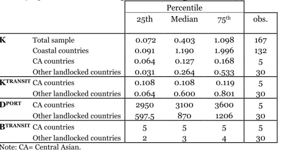
Table 3 reports the quartile values for our variables of interest, while Table 4 summarizes the disadvantages of being landlocked and having a weak infrastructure for a representative (i.e. median) Central Asian country.

Table 3: Quartile values (computed on average between 1992 and 2004) Percentile 25th Median 75th _obs. K Total sample 0.072 0.403 1.098 167 Coastal countries 0.091 1.190 1.996 132 CA countries 0.064 0.127 0.168 5

Other landlocked countries 0.031 0.264 0.533 30

KTRANSIT _{CA countries 0.108 0.108 0.119 5}

Other landlocked countries 0.064 0.600 0.801 30

DPORT _{CA countries 2950 3100 3600 5}

Other landlocked countries 597.5 870 1206 30

BTRANSIT _{CA countries 5 5 5 5}

Other landlocked countries 2 3 4 30

Note: CA= Central Asian. Source: Authors’ calculations.

We compute how the volume of trade of this median Central Asian country will change depending on the levels of its own and/or of its transit countries’ infrastructure, on the extra transport costs due to overland transport distances and on the ability of a landlocked country to negotiate access to the sea.

To summarize, an improvement in the internal infrastructure of each Central Asian country from the level of the median Central Asia country to that of the best 25th _{percentile of other landlocked countries increases exports and imports by}

6.5% and 8.6% respectively.28 _{An improvement in K to the level of the median}

coastal country generates an increase in exports and imports of 14.5% and 19.6% respectively. The impact of the infrastructure of an individual country is not particularly significant29 _{but it would appear that the infrastructure of transit}

countries is of greater importance for the international trade of landlocked countries. This hypothesis is confirmed by the results presented in this Section. An improvement in transit country infrastructure to the level of the best 25th

percentile of other landlocked countries, by cutting transit transport costs, increases the representative Central Asian exports flow by 52%. Where all transit transport costs are removed, as for a median costal country, representative Central Asian export flows would be increased by 90%.

28 _{Maintening all other variables at the level of the representative Central Asian country (median}

value).

29 _{Not specific to landlocked countries, as the associated coefficient is the same for all countries in}

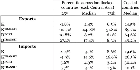
Table 4: Simulations of trade changes for a median Central Asian country

Percentile across landlocked countries (excl. Central Asia)

Coastal countries 25th _{Median 75th Median} Exports K -1.8% 2.4% 6.5% 14.5% KTRANSIT _{-12.7% 44. 8% 51.8% 89.7%} DPORT _{10.8% 8.2% 6.0% 64.6%} BTRANSIT _{27.1% 17.4% 8.3% 49.2%} Imports K -2.4% 3.1% 8.6% 19.6% KTRANSIT _{-4.9% 14.6% 16.6% 26.5%} DPORT _{5.6% 4.3% 3.2% 30.4%} BTRANSIT _{5.7% 3.1% 1.3% 10.1%}

Note: The construction of the trade changes reported in the above table is as follows. We first calculate the predicted trade for a median Central Asian country (on average over 1992-2004), denoted MCA. We then compute the predicted trade, denoted Mpred allowing K, KTRANSIT, DjPORT, and

BTRANSIT _{to vary successively, while keeping all other variables at the level of the representative}

Central Asian country (median value). The change reported in the table is 100(Mpred/MCA –1). The

values of K, KTRANSIT_{, Dj}PORT_{, and B}TRANSIT _{chosen for the simulations are the quartile values across}

the landlocked countries (excluding Central Asia) and the median value across coastal countries. All the explanatory variable values used in these calculations are reported in Table 3. The gravity specifications are found in column 2 of Table 3 and columns 6, 8 and 10 of Tables 1 and 2.

Source: Authors’ calculations.

Other dimensions of landlockedness are also great impediments to the trade of Central Asian countries. Hence, diminishing the extra overland costs (proxied by the distance to the nearest port) or enhancing the ability of a landlocked country to negotiate sea access compared to others landlocked countries would significantly increase Central Asian trade.

5

5..CCOONNCCLLUUSSIIOONN

The empirical evidence reviewed in this paper suggests that building roads is probably not by itself the best way of alleviating the burden of landlockedness. We find that three factors really matter, none of which is directly linked to the landlocked CACs’ own infrastructure: overland transportation costs, bargaining power with transit countries and the infrastructure of the latter. Moreover, of the three components of trade costs arising from landlockedness, only the transit countries’ infrastructure is specific to Central Asia. Improvements in transit- country infrastructure raise trade three times more for Central Asian countries than for other landlocked countries. By contrast, distance to port and the number of coastal neighbours a proxy for competition between transit corridors have the same impact for Central Asian countries and for other landlocked countries. Although these estimates are subject to the usual caveats, their policy message is clear. First, transit infrastructure is a regional public good and should be